cond-mat/9508xxx
A reaction-diffusion model for the hydration/setting of cement

Abstract

We propose a heterogeneous reaction-diffusion model for the hydration and setting of cement. The model is based on diffusional ion transport and on cement specific chemical dissolution/precipitation reactions under spatial heterogeneous solid/liquid conditions. We simulate the spatial and temporal evolution of precipitated micro structures starting from initial random configurations of anhydrous cement particles. Though the simulations have been performed for two dimensional systems, we are able to reproduce qualitatively basic features of the cement hydration problem. The proposed model is also applicable to general water/mineral systems.

I Introduction

In the present paper we propose a heterogeneous reaction-diffusion model for the hydration and setting of cement. The proposed model is based on the experimental observation that cement hydration can be described by a dissolution/precipitation mechanism [1, 2, 3, 4, 5].

The elementary aspects of the cement hydration/setting process on a mesoscopic length scale can be characterized as follows. At the initial stage cement particles or powder (in our case tricalcium silicate, $C_{3}S\equiv Ca_{3}SiO_{5}$) are mixed well with the solvent (water). Rapidly after mixing the dissolution reaction of the cement particles starts. Its principal reaction products are ions which are mobile and may diffuse into the bulk of the solvent (in our case $Ca^{2+}$ , $OH^{-}$ and $H_{2}SiO_{4}^{2-}$ ions). At this stage the ion concentrations in the bulk of the solvent are very low and, as a consequence, one finds strong ion fluxes from the dissolution front away into the solvent. However, for a given temperature and pressure the ion concentrations can not take arbitrary high values. Rather, the ion concentrations are bounded by finite solubility products above which solid phases start to precipitate from the solution. There are two associated precipitation reactions: a) the precipitation of calcium hydro-silicate sometimes referred as ‘cement gel’ ($C_{1.5}SH_{2.5}\equiv(CaO)_{1.5}\,(SiO_{2})\,(H_{2}O)_{2.5}$) and b) the precipitation of calcium hydroxide or ‘Portlandite’ ($CH\equiv Ca(OH)_{2}$)[3]. While the growth of the cement gel is the basis for the whole cement binding process, the growth of Portlandite mainly happens in order to compensate for the accumulation of $Ca^{2+}$ and $OH^{-}$ ions in solution (see below).

The process of cement dissolution, ion transport, and cement gel/Portlandite precipitation is usually referred as ‘cement hydration’. This process is to a high extent heterogeneous in the sense, that starting from initially random cement particle positions dissolution and precipitation reactions change the physical (boundary) conditions for the ion transports themselves. This is due to the fact that the diffusion within the solid phases can be neglected relative to the solvent one.

Coupled chemical dissolution/precipitation reactions are well known since a long time in geology and geochemistry. As such kind of processes are fundamental for water/mineral systems some effort has been undertaken to modellize such systems [6, 7]. The approaches differ methodologically and focus on different physical and chemical aspects. Ref. REFERENCES considers the ion transport problem for a single, solubility controlled, dissolution/precipitation reaction employing a one dimensional cellular automaton approach. A chemically more detailed approach of water/mineral interactions includes considerations on the influence of nucleation, electro chemistry and temperature on chemical reaction rates, however, without considering a transport equation[7].

Recently, a relatively simple stochastic cellular automaton model for cement hydration/setting has been proposed [8]. Therein it has been tacitly assumed that ion transport is not relevant for the hydration process above a certain mesoscopic length scale (‘pixel size’). Furthermore, in this model hydrate ‘pixels’ perform a random walk until they touch another solid ‘pixel’, where they then stick [8]. In contrast to this we position our deterministic model into the ‘opposite’ direction: mass transport happens due to diffusion of ions, and the hydrates are regarded as immobile.

In Sec. II we give a detailed description of the employed model. We consider heterogeneity aspects in Sec. II A, chemical aspects in Sec. II B and transport aspects in Sec. II C. Sec. III contains first results. We present some images of calculated cement micro structures, which comprehensively demonstrate basic features and capabilities of the present approach. We consider parametric plots for the mean ion concentrations, known in cement literature as ‘kinetic path approach’ and compare our findings with experimental results [9]. Following this we investigate the variation of the maximum average silica concentration in solution for various chemical reaction rate constants. Finally we present curves for the hydration advancement in time for two different sets of reaction rate constants. In Sec. IV we summarize and give some ideas about future work.

II The Model

In the following we describe the proposed reaction diffusion model for the hydration and setting of cement in more detail.

We will first discuss how to quantitatively describe the heterogeneities and outline some general features of the employed model. Following this we will summarize the dissolution/precipitation reactions and the employed reaction rate laws. Finally some physical aspects of the ion transport in the solvent are discussed. The later one represents the physical coupling between the dissolution and precipitation reactions.

A Heterogeneity aspects

We consider a discrete reaction-diffusion model in space and time. The physicochemical system can be regarded as being composed of ‘sufficient’ small volume elements $V=\Delta x^{3}$ with $\Delta x$ typically between $10^{-6}m$ and $10^{-4}m$. The initial configuration is determined from a digitized micro graph image as follows: the micro graph is immediately taken after mixing at time $t_{0}$, one can assume to find only the solid phase $C_{3}S$ and water. By measuring the occupied volumes $V_{i}^{(\alpha)}$ of the phase $\alpha$, ($\alpha=aq,C_{3}S$), in each cell $i$ using an image processing system, one determines the initial distribution of mole numbers $n_{i}^{(\alpha)}(t_{0})$ according to $n_{i}^{(\alpha)}(t_{0})=V_{i}^{(\alpha)}(t_{0})/v^{(\alpha)}$. The $v^{(\alpha)}$ are known molecular volumes for room temperature, see Table I. In general, such a micro graph shows cement particles of different sizes immersed in water. Because each cell volume is completely filled with solid and solvent phases, one can calculate the solvent volume of cell $i$ at any time step from the corresponding solid volume(s),

$$V_{i}^{(aq)}(t)=V-\sum_{\alpha\neq aq}n_{i}^{(\alpha)}(t)v^{(\alpha)}.$$ (1)

This is a very equation, because ion concentrations are usually calculated with respect to the actual solvent volume $V_{i}^{(aq)}(t)$. The physical constraints of Eq.(1) are that the chemical reactions must be sufficiently slow in comparison to the solvent flow. Furthermore, it is tacitly assumed that the whole system is connected to an external water reservoir in such a way that the solid phases do not hinder the flow.

In a given volume element the dissolution/precipitation reactions will, in general, not instantaneously go to completion. The solvent volume in each cell will rather increase/decrease continuously, defining a solvent distribution field,

$$\varepsilon_{i}^{(aq)}(t)=V_{i}^{(aq)}(t)/V.$$ (2)

The solid phase volume fractions $\varepsilon_{i}^{(\alpha)}(t)$ are defined analogously.
We believe in fact that the volume fractions $\varepsilon_{i}^{(\alpha)}(t)$, reflecting the actual solvent/solid distribution in the system, are sufficient to characterize most of the aspects of the hydration process on a macroscopic length scale.
Though we do not have information about these distributions on a length scale smaller than $\Delta x$ we will assume that the reactants are homogeneously distributed in each volume element. The volume fractions may then be interpreted as probabilities to find at a random position within cell $i$ the reactant $\alpha$.

B Chemical aspects

In the following we will summarize the considered dissolution/precipitation reactions and the employed reaction rate laws. During the course of the simulation it may happen that the reaction flux, as calculated from the kinetic equations, does exceed the available amounts of chemical reactants in a given cell. We therefore check at each time step and for each chemical reaction if there exists a limiting reactant. If this happens, we define the reaction flux through the amount of the available limiting reactant.

1 $C_{3}S$ dissolution

The $C_{3}S$ dissolution reaction is a spontaneous and exothermic surface reaction which happens at the $C_{3}S$-solvent interface(s) [3]. It can be considered as irreversible,

$$C_{3}S_{(s)}+3H_{2}O_{(\ell)}\stackrel{{\scriptstyle k_{1}}}{{\rightharpoonup}}3Ca^{2+}_{(aq)}+4OH^{-}_{(aq)}+H_{2}SiO_{4(aq)}^{2-}.$$ (3)

Here $k_{1}$ denotes an appropriate surface reaction constant in units of $mol\,m^{-2}\,s^{-1}$.
Chemical reactions must be considered as local, i.e., each volume element is acting as a small and independent chemical reactor as long as no transport occurs. However, for a pronounced dissolution reaction in a given cell one has also to consider the possible reaction amounts originating from the interfaces with its neighboring cells. This can be done by allowing cement dissolution in cell $i$ through the electro chemicalsolvent of that cell and through a fraction $\gamma$ of the solvent of the neighboring cells $j$,

$$\nu_{1}^{(\alpha)}\,d\xi_{i,1}(t)=\nu_{1}^{(\alpha)}\,k_{1}\,\Delta t\,\Delta x^{2}\,\bigl{(}p_{ii}+\gamma\sum_{j=nn(i)}(p_{ij}-p_{ii})\bigr{)}.$$ (4)

Here $\nu_{1}^{(\alpha)}$ denote the stoichiometric numbers of species $\alpha$ in reaction (3), see Table I. The changes in mole numbers of species $\alpha$ in cell $i$ in a time intervall $\Delta t$ due to this reaction are denoted by $\nu_{1}^{(\alpha)}\,d\xi_{i,1}(t)$. The sum on the right hand has to be taken over all next nearest neighboring cells of cell $i$, as indicated by $j=nn(i)$. The first term $p_{ii}=\varepsilon_{i}^{(C_{3}S)}\varepsilon_{i}^{(aq)}$ in Eq.(4) describes the dissolution within cell $i$ ($\gamma=0$) due to a ‘typical’ reaction interface. It can be understood as a probability to find the two reactants, $C_{3}S$ and water, in contact at an arbitrary chosen point within cell $i$. The ‘chemically active interface’ between cell $i$ and $j$ is given by $p_{ij}\Delta x^{2}=\Delta x^{2}\varepsilon_{i}^{(C_{3}S)}\varepsilon_{j}^{(aq)}$. The constant $\gamma$ controls the degree of dissolution due to this interface(s). We have used a value $\gamma=1/8$ in our simulations, yielding comparable reaction rates from inner and outer cell surfaces. The determination of the reaction interfaces in terms of cement and water volume fractions is similar to the degree of surface coverage used in Langmuir absorption theory [10]. However, the absorption of water on the cement’s surface and the desorption of ions from this surface are not necessarily the rate determining steps. In fact, the dissolution reaction (3) involves various physical and subprocesses [5] which will not be considered here.

2 $CSH$ dissolution/precipitation

The precipitation of $C_{1.5}SH_{2.5}$ is an endothermic reaction which can be considered as reversible [3],

$$C_{1.5}SH_{2.5(s)} \stackrel{{\scriptstyle k_{2}}}{{\rightleftharpoons}} H_{2}SiO_{4(aq)}^{2-}$$ (5)

$$+ 1.5Ca^{2+}_{(aq)}+OH^{-}_{(aq)}+H_{2}O_{(\ell)},$$ (6)

having a forward (dissolution) rate constant $k_{2}$ (in units of $mol\,m^{-2}\,s^{-1}$).

We note, that the $CSH$ precipitation, i.e., the backward reaction in Eq.(5) is the main reaction in this balance equation. The reactants and products are considered to have a fixed stoichiometry. However, it is known from experimental data that the stoichiometry of $C_{x}S_{y}H_{z}$ can be rather variable (‘solid solution’) [2]. We will not include these complications into the model. Instead we consider a fixed and typical calcium/silica ratio equal to $1.5$.

In equilibrium the $C_{1.5}SH_{2.5}$ dissolution/precipitation reactions are controlled by an empirical value of solubility, giving the maximum amount of solid one can dissolve in aqueous solution at a given temperature (room temperature) and pressure (normal pressure). Employing this empirical solubility constant one can directly determine the equilibrium solubility product, $S_{2}^{equi}=S_{2i}|^{equi}=(Ca^{2+})_{i}^{1.5}(OH^{-})_{i}(H_{2}SiO_{4}^{2-})_{i}|^{equi}\approx 1.2\times 10^{-9}\,mol^{3.5}\,liter^{-3.5}$, comp. Table I. The square brackets denote the ion concentrations with respect to the available solvent, i.e., $(Ca^{2+})_{i}=n_{i}^{(Ca^{2+})}/V_{i}^{(aq)}$ etc.. When in a given cell the ion product is larger than the solubility product, locally precipitation happens. If it is lower, $C_{1.5}SH_{2.5}$ becomes dissolved. The $CSH$ dissolution is only marginal and for this reason we will employ for the rate of dissolution a simpler expression than for the $C_{3}S$ dissolution reaction.

We assume that the dissolution reaction in cell $i$ is proportional to the typical reaction interface $\Delta x^{2}\varepsilon_{i}^{(aq)}$ with the dissolution constant $k_{2}$ as the constant of proportionality. The precipitation reaction is assumed to be proportional to the reaction interface and proportional to the ion product $S_{2i}$, as defined above. The rate constant of the precipitation reaction can be eliminated, by use of the equilibrium condition, $d\xi_{i,2}=0$. We have employed the following rate equation,

$$\nu_{2}^{(\alpha)}\,d\xi_{i,2}(t)=\nu_{2}^{(\alpha)}\,k_{2}\,\Delta t\,\Delta x^{2}\,\varepsilon_{i}^{(aq)}\bigl{(}1-\frac{S_{2i}}{S_{2}^{equi}}\bigr{)}.$$ (7)

The stoichiometric numbers again are denoted by $\nu_{2}^{(\alpha)}$, see Table I, and the change in mole numbers of species $\alpha$ due to this reaction is $\nu_{2}^{(\alpha)}\,d\xi_{i,2}(t)$.

3 CH dissolution/precipitation

The precipitation of calcium hydroxide accompanies the $CSH$ precipitation. This is because the $CSH$ precipitation does not consume the ions in the same proportions as they are released due to $C_{3}S$ dissolution. The non-reacted $Ca^{2+}$ and $OH^{-}$ ions soon begin to accumulate in solution, until the solubility of $CH$ is exceeded. However, the precipitation of $CH$ and $CSH$ are, in general, not simultaneous because the corresponding solubilities are very different, comp. Table I. The dissolution/precipitation of $CH$ can be considered as reversible,

$$CH_{(s)}\stackrel{{\scriptstyle k_{3}}}{{\rightleftharpoons}}Ca^{2+}_{(aq)}+2OH^{-}_{(aq)},$$ (8)

having a dissolution constant $k_{3}$ ($mol\,m^{-2}\,s^{-1}$).

The corresponding solubility product for $CH$ is defined as $S_{3}^{equi}=S_{3i}|^{equi}=(Ca^{2+})_{i}(OH^{-})_{i}^{2}|^{equi}\approx 3.3\times 10^{-6}\,mol^{3}\,liter^{-3}$ which is about three orders of magnitude larger than $S_{2}^{equi}$, see Table I,

$$\nu_{3}^{(\alpha)}\,d\xi_{i,3}(t)=\nu_{3}^{(\alpha)}\,k_{3}\,\Delta t\,\Delta x^{2}\,\varepsilon_{i}^{(aq)}\bigl{(}1-\frac{S_{3i}}{S_{3}^{equi}}\bigr{)}.$$ (9)

In all other respects the $CH$ reaction is treated analogously to the $CSH$ dissolution/precipitation reaction.

4 Chemical shrinkage

One can write down from Eqs.(3), (5) and (8) the net reaction for the cement hydration process,

$$C_{3}S_{(s)}+4H_{2}O_{(\ell)}\rightharpoonup C_{1.5}SH_{2.5(s)}+1.5CH_{(s)}.$$ (10)

Calculating for the above equation the occupied volumes for one mole one finds for the left side approximately $144\,cm^{3}$ and for the hydrate products $130\,cm^{3}$, comp. Table I. Hence, the reaction products occupy a volume around 10% smaller than the reactants (including solvent). This effect, which is typical for hydraulic binders, is termed ‘chemical shrinkage’ or Le Chatelier effect. It is responsible for the transition of cement suspensions or pastes having a finite viscosity and zero elastic moduli to rigid hydrated cement having an infinite viscosity and finite elastic moduli. Wherever topologically possible water flow will try to compensate for the loss of volume. However, in the course of an experimental cement setting and hardening (rigidification) process available solvent flow paths may vanish and volume loss becomes partially compensated building up mechanical deformations (stresses) within the solid phase agglomerate. In turn these stresses influence the reaction rates (which in general are pressure dependent) in a complex manner [4]. The appearence of voids (pores) on the submicron scale is experimentally also well established [1].

We will not modellize such complex problems as mechanical stresses, solvent cavitation and solvent flow due to chemical shrinkage in our present approach.

Instead we will assume throughout all calculations that the solvent is able to balance the chemical shrinkage for all time steps and for all volume elements according to Eq.(1). This assumption is equivalent to the introduction of local source terms for water, i.e., the hydrating system is connected to an external water reservoir in an appropriate way.

We would like to point out that Eq.(10) is an overall reaction which per definition only holds for an isolated system. On the other hand one cannot treat the volume elements as chemically isolated, simply because of the ion fluxes going through the elements. This and the different values for the $CSH$ and $CH$ solubilities imply in general locally non-congruent precipitation reactions. As a consequence one cannot simply ‘replace’ one dissolved unit volume of $C_{3}S$ by 1.7 unit volumes $CSH$ and 0.6 unit volumes $CH$ as has been proposed in [8].

C Transport aspects

It is known from experiments that ion transport due to diffusion is fundamental in cement chemistry, because of very strong ion concentration gradients close to the dissolving $C_{3}S$-solvent interface(s). In general one should consider the convective diffusion equation, however, this would imply to solve the hydrodynamic equations. In the present paper we consider the usual diffusion equation with local, appropriately defined transport coefficients. It is in the context of the investigated problem useful to consider only the ion diffusion within the solvent. For convenience we document in Table I the diffusion constants $D^{(\alpha)}$ as calculated from the electric mobilities at room temperature and normal pressure for infinite dilution. The solids and the solvent’s diffusion constants are set to zero [11]. This allows a relatively compact notation for the equations of continuity,

$$\Delta n_{i}^{(\alpha)} = \frac{\Delta t}{\Delta x^{2}}V\sum_{j=nn(i)}\bigl{(}D_{ij}^{(\alpha)}c_{j}^{(\alpha)}-D_{ij}^{(\alpha)}c_{i}^{(\alpha)}\bigr{)}$$ (11)

$$+ \sum_{k=1}^{3}\nu_{k}^{(\alpha)}\,d\xi_{i,k}.$$ (12)

The second term on the right side of Eq.(11) represents the already known source term due to the chemical reactions Eqs.(4), (7) and (9). The $D_{ij}^{(\alpha)}$ are the transport coefficients, that depend on the solvent volume fractions (porosities) of the cells involved in the diffusion process, $D_{ij}^{(\alpha)}=D^{(\alpha)}\varepsilon_{i}^{(aq)}\varepsilon_{j}^{(aq)}$. The ion concentrations are taken with respect to the actual solvent volume, i.e., $c_{i}^{(\alpha)}=n_{i}^{(\alpha)}/V_{i}^{(aq)}$. We have employed periodic boundary conditions in all calculations.

The general formulation of the ion transport problem in cement chemistry involves various subproblems which we will not consider at this stage of modelization, as there are the transport due to

1 Heat conductance

The cement dissolution reaction is strongly exothermic. Analogous to the concentration gradients one finds near the various dissolution fronts strong temperature gradients, leading to non isothermal solvent flow fields, with its complications. The heat redistribution is probably also of direct importance for the dissolution/precipitation reactions, because their reaction constants as well as the corresponding solubility products usually depend very sensitively on the temperature. We will neglect this possible effects in our approach assuming an overall constant room temperature, $T_{0}=298$ Kelvin.

2 Electrostatic interactions

Because one is dealing with the transport of electrically charged particles, one must consider, in general, Poisson’s equation for the electrostatic potential in order to determine the resulting ion mobilities due to their electric field. We will neglect in our simulations all electrostatic interactions. Furthermore, all chemical rate calculations are done in terms of molar concentrations and not in terms of ‘chemical activities’ (which is equivalent in the limit of infinite dilution). Hence we will treat the ions in solution as uncharged particles throughout all calculations.

3 Solvent flow

This is possibly of importance for the overall hydration process, because the solvent has to move during the dissolution/precipitation reactions accordingly, in order to compensate for the loss/gain of solid volume, creating advective ion fluxes. For an infinite, plane cement-water interface one might argue that the solvent flow is always perpendicular to the interface. Under this particular conditions it can be shown by scaling arguments that advective ion transport is unimportant relative to the diffusion transport, because of the relatively low molecular volume of cement, comp. Table I. However, in a finite heterogeneous system solvent flows tangential with respect to the interfaces are also expected and the argument given above is limited. In principle one has to consider the equations of hydrodynamics for this purpose. However, this moving boundary problem is complex and we will not consider it in this form here. Instead we will determine the spatial and temporal solvent distribution $V_{i}^{(aq)}(t)$ according to Eq.(1).

III Results

From a general point of view cement hydration can be regarded as a heterogeneous (non equilibrium) solid phase transformation forming from an anhydrous solid phase two hydrated solid phases[12]. In contrast to known solid-solid phase transformations for example in metallic alloys, cement hydration bases strongly on the presence of a solvent phase (mostly water). The solvent controlls the transformation in a twofold sense: it is directly part of the chemical reactions and on the other hand it controlls the ion transport to a very large extent.

The complexity of the problem and the features of the present approach are most convenient illustrated by Fig. 1. Therein we show the solid volume fractions of anhydrous cement, $\varepsilon^{(C_{3}S)}$ (left side), and of hydrated cement, $\varepsilon^{(CSH)}$ (right side), for three different hydration times (a) $t=1500\,s$, (b) $t=2500\,s$ and (c) $t=5000\,s$. The occupied volume fractions are color coded ranging from blue (0-20%), cyan (20-40%), green (40-60%) over yellow-orange (60-80%) to red (80-100%). The calculated micrographs Fig. 1a-c show, as expected, spatially inhomogeneous nucleation and growth of $CSH$ hydrate. The hydrate precipitation and the associated growth of hydrate surface layers surrounding dissolving cement particles is relatively slow. However, in Fig. 1b one especially observes that the rate of $CSH$ precipitation is spatially strongly varying (notice the red and cyan spots in the right image). This reflects the spatial fluctuations in chemical reactivities (local $C_{3}S$ surface/volume ratio), i.e., the reactivity of a ‘fjord’ is higher than that of a big ‘lake’. Supported by experimental observations it has been argued that cement particle surfaces close to each other may indeed act as very strong inhomogeneities leading to localized $CSH$ nucleation forming ‘bridges’ between adjacent particles [13]. Our micrographs confirm this picture. We note, that the proposed model does not include any (auto-)catalytic effect of $CSH$ on its growth yet, compare Eq. (7). This point is intensively studied at the moment.

As the hydrate precipitation/dissolution reaction rates depend on the local supersaturation values, the interesting question arises how global characteristic points of the cement hydration kinetics can be defined. In a recent experimental work it has been proposed to characterize different kinetic regimes occuring during the $C_{3}S$ hydration by means of parametric plots of ‘typical’ calcium versus silicate concentrations as estimated from calorimetric or conductimetric measurements (‘kinetic path approach’)[9]. The experiments have been conducted employing stirred diluted $C_{3}S$ suspensions having a water/cement weight ratio between $10$ and $50$. However, to obtain typical quantities of such diluted suspensions employing numerical simulations one would have to consider very large systems. Instead we will compare the experimental suspension data with numerical cement paste data having a water/cement ratio close to the practically important value $0.5$.

For convenience we reproduce in Fig. 2 some of the experimental data $(\diamond)$ of Ref. REFERENCES. Initially one finds an ‘inductive’ cement dissolution period (period $AB$ in Fig. 2). During this period the bulk solution is everywhere undersaturated with respect to $CSH$ and $CH$, the concentration gradients close to the cement particles are very high, and ions rapidly distribute into the bulk solvent. We have observed in our simulations that $CSH$ is already formed during the ‘induction’ period, however, to a very low extent. Because of the initially very high concentration gradients the ion products exceed the $CSH$ solubility only in a very thin layer surrounding the cement particles. As the ions cummulate in solution the thickness of this precipitating layer increases due to the broadening of the ion distributions.

The precipitation counteracts the further increase in silica concentration both by chemical reaction and by decreasing the cement particles surface permeability. In result the silica concentration passes through a maximum (point $B$ in Fig. 2), which might be interpreted as a global measure for the onset of $CSH$ precipitation. During the period $BC$ the silica concentration decreases, while the calcium and hydroxyl concentrations continue to increase as the $CSH$ precipitation consumes only a fraction of these ions, see Eqs. (3) and (5).

Typically after a couple of hours the solution becomes oversaturated with respect to calcium hydroxide $CH$ (point $C$ in Fig. 2). Both hydrates precipitate very slowly (experimentally several weeks between point $C$ and $D$), lowering both calcium and hydroxyl concentrations. Point $D$ corresponds to the state after infinite hydration time terminating the shown curve. The progress in time is indicated by arrows. Our numerical results $(+)$ are in reasonable agreement with the experimental data $(\diamond)$. We have observed that calculated positions and values for point $C$ depend a) on the employed initial water/cement weight ratio and b) on the three reaction rate constants $k_{1}$, $k_{2}$ and $k_{3}$ in a rather complex manner. Contrary to this point $B$ is found to depend only slightly on the relative reaction rate constant $k_{1}/k_{2}$ over four orders of magnitude, see Fig. 3a. A consequence of the much smaller solubility of $CSH$ as compared to the second hydrate $CH$ is that in the period $AB$ only two chemical reaction are operative. Reaction Eq. (8) is inoperative. For $k_{1}/k_{2}$ ranging between $0.1$ and $10$ the maximum silica concentrations take constant values of about $1\,mmol/liter$ while for $k_{1}/k_{2}=10^{3}$ we find $\approx 3\,mmol/liter$. We have also performed simulations for similar $k_{1}/k_{2}$ values employing different absolute reaction rate constants, see Fig. 3a. We find a relatively good data collapse over four orders of magnitude. This result is important insofar as the reaction rate constants have not been experimentally measured yet. In Fig. 3b we plot the momentaneous calcium concentration versus the silica concentration at point $B$ for various reaction rate constants. The data are centered around a straight line of slope $1/3$. Comparison of this result with the stoichiometric coefficients in Eq. (3) shows that the silica/calcium ratio of ions is determined by the dissolution reaction.

The characterisation of the temporal advancement of the hydration process is an important problem. We show in Fig. 4 some preliminary results for the time dependence of the mean volume fraction $\langle\varepsilon^{(CSH)}\rangle$ of the cementious hydrate $CSH$. For ‘moderate’ reaction constants $(\diamond)$ the hydration is found to be relatively slow, i.e., after $70\,hours$ of hydration we find only $10\%$ $CSH$. This value is approximately two times lower than the experimental one observed by NMR[14]. We note that both the hydration curve $(\diamond)$ in Fig. 4 and the parametric curve $(+)$ in Fig. 2 belong to the same simulation. Apparently the hydration advancement for ‘moderate’ reaction rates is nearly constant in time, see curve $(\diamond)$ in Fig. 4. For comparison we also show in Fig. 4 a hydration curve for ‘fast’ hydration $(+)$. After a few minutes of ‘induction’ period the hydration rapidly accelerates and goes already after $1\,hour$ to completion (remaining $C_{3}S$ less than $1\;\%$). This process is much to fast and it leads to typical ion concentrations of $mol/liter$ which are unrealistic high.

As long as the reaction rate constants have not been estimated from experiments yet one main difficulty in the modellization of cement hydration consists in finding appropriate values for the rate constants, which do not contradict experimental measurements of mean ion concentrations and hydration advancement. However, the experimental results belong to hydration in space while our calculations correspond to two dimensional hydration. This point is being currently investigated.

IV Conclusions

We have presented a general, heterogeneous reaction-diffusion model for solid phase transformation due to chemical dissolution/precipitation reactions. The model has focussed on the important industrial problem of Portland cement hydration though it is more generally applicable to water/mineral systems.

We have tried to develop an ‘open’ approach based on physical and chemical considerations (mainly the laws of mass conservation and mass action). The model includes in its present form on a coarse grained length and time scale the full spatial distribution of solid and liquid phases, the three main chemical dissolution/precipitation reactions, and the transport of ions due to diffusion. The proposed approach naturally allows to include for a varity of more or less important phenomena depending on imposed conditions such as solvent flow effects, electrochemical effects, exothermic effects including heat conduction, pressure effects, inert filler effects etc..

We have tried to incorporate a reasonable amount of specific information about the cement hydration into the investigated model such as the stoichiometry and kinetics of Portland cement dissolution, the precipitation/dissolution of the main cementious hydrate (CSH) and of Portlandite (CH), their approximate solubilities and molecular volumes, approximate values for the ion diffusivities in aqueous solution, and initial conditions for water immersed cement particles (sizes and spatial positions).

The presented results demonstrate considerable richness and complexity of the cement hydration phenomenon close to controlled experimental situations.

We have presented some calculated cement micro structures as they evolve in time. Nucleation and growth of hydrates is found to be strongly heterogeneous in agreement with experimental observations. The problem of ‘autocatalytic’ effects on the precipitation processes needs further investigation.

The presented parametric plots for the average concentrations of ions in solution are in qualitative agreement with recent indirect experimental observations made for stirred cement suspensions[9]. The calculated maximum silica concentrations and their corresponding calcium concentrations are in reasonable quantitative agreement with experimental values. For high dissolution and low precipitation rate constants we find unacceptable high ion concentrations of order $mol/liter$. One way to circumvent this problem would be the introduction of a finite solubility for $C_{3}S$ in Eq. (4), however, such a solubility constant has not been experimentally determined yet.

Furthermore we have investigated the variations of the maximum silica concentrations for various reaction rate constants. The concentrations are found to vary only slightly with the relative reaction rate constant $k_{1}/k_{2}$ over four orders of magnitude. It would be very interesting to see how the second characteristic hydration point (point $C$ in Fig. 2) depend on the initial water/cement ratio and on the employed reaction rate constants.

Finally we presented first results on overall hydration curves. This curves are not very realistic yet. It would be very helpfull to have experimental order of magnitude estimates for the three (unknown) reaction rate constants.

For future work we are planning to conduct calculations in three dimensions with improved kinetic equations.

TABLE I.: Stoichiometric numbers $\nu_{1}^{(\alpha)}$, $\nu_{2}^{(\alpha)}$ and $\nu_{3}^{(\alpha)}$ of the chemical reactions Eqs.(3), (5) and (8) respectively. The last three colums give the molecular volumes, the diffusion constants and the solubilities at room temperature and normal pressure.

Species		Stoichiometric numbers		Molecular volume	Diffusion constant	Solubility
$\alpha$	$\nu_{1}^{(\alpha)}$	$\nu_{2}^{(\alpha)}$	$\nu_{3}^{(\alpha)}$	[$10^{-3}\;liter/mol$]	[$10^{-10}\;m^{2}/s$]	[$10^{-3}\;mol/liter$]
$H_{2}O$	$-3$	$-1$	$0$	$18.01$	$0$	—
$C_{3}S$	$-1$	$0$	$0$	$73.1^{~{}(b)}$	$0$	$\infty^{~{}(f)}$
$C_{1.5}SH_{2.5}$	$0$	$1$	$0$	$80.40^{~{}(c)}$	$0$	$2.4^{~{}(d)}$
$CH$	$0$	$0$	$1$	$33.07^{~{}(a)}$	$0$	$20.2^{~{}(a)}$
$Ca^{2+}$	$3$	$-3/2$	$-1$	—	$7.9^{~{}(e)}$	—
$OH^{-}$	$4$	$-1$	$-2$	—	$53.0^{~{}(e)}$	—
$H_{2}SiO_{4}^{2-}$	$1$	$-1$	$0$	—	$5.0^{~{}(f)}$	—

${}^{~{}(a)}$ H.F.W. Taylor, Cement Chemistry, (Academic Press, London, 1990), pp. 125; ${}^{~{}(b)}$ ibid, p. 15; ${}^{~{}(c)}$ ibid, p. 152, we assume for the calculations a density of $2.35\,g\,cm^{-3}$; ${}^{~{}(d)}$ We have calculated this value from the supersaturation concentrations of calcium and silicate ions, as reported in Ref. REFERENCES; ${}^{~{}(e)}$ R.A. Alberty and R.J. Silbey, Physical Chemistry, (Wiley&Sons, New York, 1992), pp. 839; ${}^{~{}(f)}$ Measured values are not known to us.

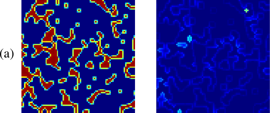
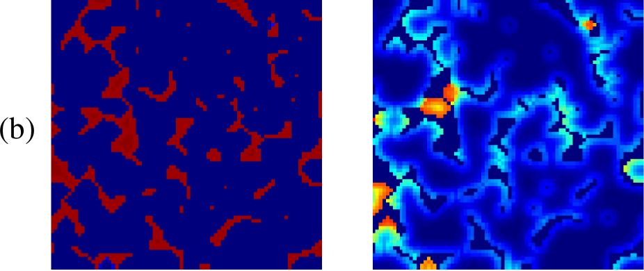
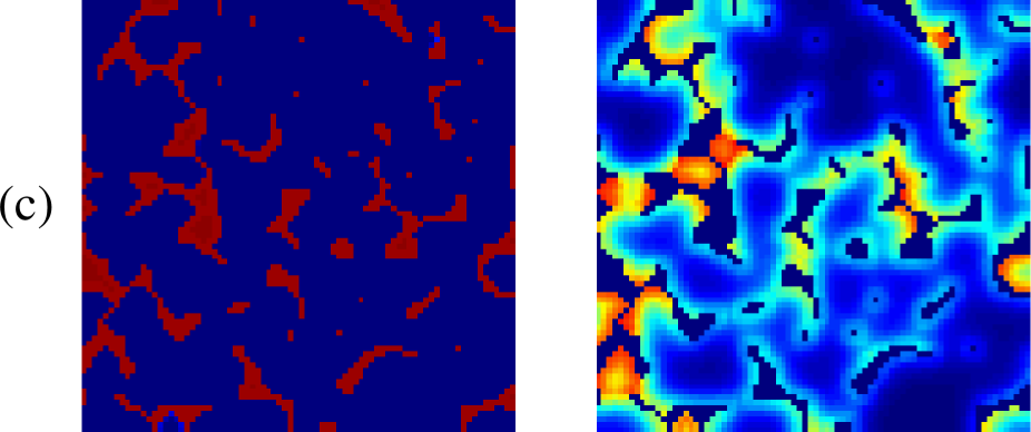
FIG. 1.: The above figures show numerically calculated cement micro structures after (a) $t=1500\,s$, (b) $t=2500\,s$ and (c) $t=5000\,s$. Images on the left side show the unhydrated cement phase (C3S) while those on the right side represent the hydrated, precipitated cement (CSH). The colors indicate the local solid volume fractions, i.e., blue (0-20%), cyan (20-40%), green (40-60%), yellow-orange (60-80%) and red (80-100%). The initial water/cement ratio is about 0.4, the reaction rate constants are $k_{1}=10^{-3}$, $k_{2}=10^{-12}$ and $k_{3}=10^{-10}$ (in units of $mol\,m^{-2}\,s^{-1}$). The employed cell size is $\Delta x=10^{-4}\,m$, the linear system size $L=100\Delta x$, and the linear cement particle size $\ell=5\Delta x$. The time step is $0.01\,s$. All other parameters as in Table I.

FIG. 2.: Parametric plot of the evolution of silica versus calcium concentration (‘kinetic path approach’); $(\diamond)$ experimental results after Ref. REFERENCES, $(+)$ numerical results. The employed reaction rate constants are $k_{1}=5\cdot 10^{-5}$, $k_{2}=10^{-6}$ and $k_{3}=10^{-8}$ (in units of $mol\,m^{-2}\,s^{-1}$). The linear system size is $L=50\Delta x$, the cell size $\Delta x=10^{-4}\,m$ and the linear cement particle size $\ell=5\Delta x$. The employed time step is $0.1\,s$. Initial water/cement weight ratio $0.6$. All other parameters as in Table I.

FIG. 3.: Calculated silica ion concentration $(H_{2}SiO_{4}^{2-})$ at the onset of $CSH$ precipitation (corresponding to point $B$ in Fig. 2): (a) double logarithmic plot versus the relative reaction rate constant $k_{1}/k_{2}$, (b) plot against the momentaneous $(Ca^{2+})$ ion concentration. Symbols: $(\diamond)$ $k_{1}=10^{-4}\,mol\,m^{-2}\,s^{-1},\,k_{1}/k_{2}$ ranging between $1$ and $1000$; $(+)$ $k_{1}=10^{-5}\,mol\,m^{-2}\,s^{-1},\,k_{1}/k_{2}$ ranging between $0.125$ and $500$; $(\Box)$ $k_{1}=10^{-6}\,mol\,m^{-2}\,s^{-1},\,k_{1}/k_{2}$ ranging between $0.167$ and $600$; $(\times)$ $k_{1}=10^{-7}\,mol\,m^{-2}\,s^{-1},\,k_{1}/k_{2}$ ranging between $0.167$ and $0.5$. Each point corresponds to an average over $10$ configurations having an initial water/cement weight ratio of about $0.5$. All other parameters as in Fig. 2.

FIG. 4.: Double logarithmic plot of the average $CSH$ volume fraction $\langle\;\varepsilon^{(CSH)}\;\rangle$ versus hydration time $t$ for two sets of reaction rate constants: $(\diamond)$ $k_{1}=5\cdot 10^{-5}$, $k_{2}=10^{-6}$ and $k_{3}=10^{-8}$; $(+)$ $k_{1}=10^{-2}$, $k_{2}=10^{-16}$ and $k_{3}=10^{-13}$; units in $mol\,m^{-2}\,s^{-1}$. All other parameters as in Fig. 2.

REFERENCES

- [1] H.F.W. Taylor, Cement Chemistry, (Academic Press, London 1990).
- [2] P. Barret and D. Bertrandie, Journal de Chimie Physique 83, 11/12, 765-75, (1986).
- [3] D. Damidot and A. Nonat in Hydration and Setting of Cements, eds. A. Nonat and J.C. Mutin (E&F Spon, London, 1992), p. 23.
- [4] M. Michaux, E.B. Nelson and B. Vidick in Well Cementing, ed. E.B. Nelson (Schlumberger Educational Services, Housten, 1990), pp.2-1.
- [5] See for example: C. Vernet, Introduction a la Physicochimie du Ciment Portland. Deuxième partie. Chimie de l’hydratation., Technodes S.A., Groupe Ciments Francais, 1992.
- [6] T. Karapiperis, J. Stat. Phys., unpublished; T. Karapiperis and B. Blankleider, Physica D 78, 30-64, (1994).
- [7] B. Madé, A. Clément and B. Fritz, Revue de l’Institut Francais du Petrole 49, 6, (1994).
- [8] D.P. Bentz and E.J. Garboczi, Cement and Concrete Research 21, 325-44, (1991); E.J. Garboczi and D.P. Bentz, Journal of Materials Science 27, 2083-92, (1992).
- [9] D. Damidot and A. Nonat, Advances in Cement Research 6 (21), 27-35, (1994); D. Damidot and A. Nonat, Advances in Cement Research 6 (22), 83-91, (1994); D. Damidot, A. Nonat, P. Barret, D. Bertrandie, H. Zanni and R. Rassem, Advances in Cement Research 7 (25), 1-8, (1995).
- [10] R.A. Alberty and R.J. Silbey, Physical Chemistry, (Wiley&Sons, New York, 1992), pp. 839.
- [11] As aforementioned we determine the solvent volume and its mole numbers exclusively from Eq.(1). This assumption is reasonable as long as the number of solvated ions is much lower than the number of solvent molecules.
- [12] It has been reported that under very particular experimental conditions (strongly diluted suspensions) the precipitation of calcium hydroxide becomes supressed, see Ref. REFERENCES.
- [13] A. Nonat, Materials and Structures 27, 187-95, (1994).
- [14] C.M. Dobson, D.G.C. Goberdhan, J.D.F. Ramsay and S.A. Rodger, J. Mat. Sci. 23, 4108-14 (1988).