[

Superconducting Upper Critical Field near a 2D van Hove singularity

Abstract

The superconducting upper critical field $H_{c2}(T)$ of a two dimensional BCS superconductor is calculated in the vicinity of a van-Hove singularity. The zero temperature upper critical field is strongly enhanced at weak coupling when the Fermi contour coincides with van-Hove points, scaling as $H_{c2}(0)\propto T_{c}^{\sqrt{2}}$ compared to the usual result $H_{c2}(0)\propto T_{c}^{2}$. The result can be interpreted in terms of the non-Fermi liquid decay of normal state pair correlations in the vicinity of a van-Hove point.

]

The possibility of a strong enhancement of the superconducting transition temperature in the vicinity of van-Hove singularities (vHs) of electronic systems has been raised on several occasions.[2, 3] At a vHs, the Fermi velocity vanishes at points on the Fermi contour and in 2D, the density of states diverges logarithmically. While it is tempting to apply this simple model of $T_{c}$ enhancement to realizations of quasi-2D systems such as Copper-Oxide superconductors,[4, 5] it is often pointed out that three-dimensionality and scattering effects have the effect of smearing out the vHs. Also, the electron kinetic energy favors low density of states at the Fermi level and structural distortions may be expected to occur in order to push the vHs below the Fermi level.[6]

Despite these limitations, the 2D vHs provides a simple and well-understood example of a normal Fermi system which possesses anomalous normal state correlations and therefore deserves to be understood in detail. The origin of non-Fermi liquid effects in this case is the absence of a well-defined Fermi velocity scale, which is in turn due to the presence of an underlying lattice and the absence of Galilean invariance. It has recently been shown that non-Fermi liquid behavior in the normal state leads to deviations from the usual quasi-parabolic mean-field $H_{c2}(T)$ curve of Fermi liquid BCS (FL-BCS) superconductors found by Gorkov.[7, 8] Interestingly, deviations from the parabolic shape have been observed in layered superconductors,[9] including both Copper-Oxides[10] and $k\mbox{-(BEDT-TTF)}_{2}\mbox{Cu(NCS)}_{2}$.[11] As emphasized previously,[7] the mean field upper critical field is a normal state property which probes both the spatial (via the magnetic length) and energy (temperature) dependence of pair correlations. It may therefore prove an effective probe of non-Fermi liquid normal effects.

In the present paper we show that anomalous correlations in the vicinity of a 2D vHs lead to spectacular deviations from the FL-BCS result. Following the semi-classical Gorkov approach,[12, 13] the superconducting transition corresponds to the appearance of non-trivial solutions of the equation

$$\Delta({\mathchoice{{\hbox{\boldmath$\displaystyle r$}}}{{\hbox{\boldmath$\textstyle r$}}}{{\hbox{\boldmath$\scriptstyle r$}}}{{\hbox{\boldmath$\scriptscriptstyle r$}}}})=g\int d^{2}{\mathchoice{{\hbox{\boldmath$\displaystyle r$}}}{{\hbox{\boldmath$\textstyle r$}}}{{\hbox{\boldmath$\scriptstyle r$}}}{{\hbox{\boldmath$\scriptscriptstyle r$}}}^{\prime}}K_{\beta}({\mathchoice{{\hbox{\boldmath$\displaystyle r$}}}{{\hbox{\boldmath$\textstyle r$}}}{{\hbox{\boldmath$\scriptstyle r$}}}{{\hbox{\boldmath$\scriptscriptstyle r$}}}^{\prime}})e^{i[{\mathchoice{{\hbox{\boldmath$\displaystyle A$}}}{{\hbox{\boldmath$\textstyle A$}}}{{\hbox{\boldmath$\scriptstyle A$}}}{{\hbox{\boldmath$\scriptscriptstyle A$}}}}({\mathchoice{{\hbox{\boldmath$\displaystyle r$}}}{{\hbox{\boldmath$\textstyle r$}}}{{\hbox{\boldmath$\scriptstyle r$}}}{{\hbox{\boldmath$\scriptscriptstyle r$}}}})+{\mathchoice{{\hbox{\boldmath$\displaystyle A$}}}{{\hbox{\boldmath$\textstyle A$}}}{{\hbox{\boldmath$\scriptstyle A$}}}{{\hbox{\boldmath$\scriptscriptstyle A$}}}}({\mathchoice{{\hbox{\boldmath$\displaystyle r$}}}{{\hbox{\boldmath$\textstyle r$}}}{{\hbox{\boldmath$\scriptstyle r$}}}{{\hbox{\boldmath$\scriptscriptstyle r$}}}^{\prime}})]({\mathchoice{{\hbox{\boldmath$\displaystyle r$}}}{{\hbox{\boldmath$\textstyle r$}}}{{\hbox{\boldmath$\scriptstyle r$}}}{{\hbox{\boldmath$\scriptscriptstyle r$}}}^{\prime}}-{\mathchoice{{\hbox{\boldmath$\displaystyle r$}}}{{\hbox{\boldmath$\textstyle r$}}}{{\hbox{\boldmath$\scriptstyle r$}}}{{\hbox{\boldmath$\scriptscriptstyle r$}}}})}\Delta({\mathchoice{{\hbox{\boldmath$\displaystyle r$}}}{{\hbox{\boldmath$\textstyle r$}}}{{\hbox{\boldmath$\scriptstyle r$}}}{{\hbox{\boldmath$\scriptscriptstyle r$}}}}+{\mathchoice{{\hbox{\boldmath$\displaystyle r$}}}{{\hbox{\boldmath$\textstyle r$}}}{{\hbox{\boldmath$\scriptstyle r$}}}{{\hbox{\boldmath$\scriptscriptstyle r$}}}^{\prime}})$$ (1)

where $\beta$ is the inverse temperature and $g$ the pairing interaction. The magnetic field effect is included in a semi-classical form as a phase term[14] $\exp({i[{\mathchoice{{\hbox{\boldmath$\displaystyle A$}}}{{\hbox{\boldmath$\textstyle A$}}}{{\hbox{\boldmath$\scriptstyle A$}}}{{\hbox{\boldmath$\scriptscriptstyle A$}}}}({\mathchoice{{\hbox{\boldmath$\displaystyle r$}}}{{\hbox{\boldmath$\textstyle r$}}}{{\hbox{\boldmath$\scriptstyle r$}}}{{\hbox{\boldmath$\scriptscriptstyle r$}}}})+{\mathchoice{{\hbox{\boldmath$\displaystyle A$}}}{{\hbox{\boldmath$\textstyle A$}}}{{\hbox{\boldmath$\scriptstyle A$}}}{{\hbox{\boldmath$\scriptscriptstyle A$}}}}({\mathchoice{{\hbox{\boldmath$\displaystyle r$}}}{{\hbox{\boldmath$\textstyle r$}}}{{\hbox{\boldmath$\scriptstyle r$}}}{{\hbox{\boldmath$\scriptscriptstyle r$}}}^{\prime}})]({\mathchoice{{\hbox{\boldmath$\displaystyle r$}}}{{\hbox{\boldmath$\textstyle r$}}}{{\hbox{\boldmath$\scriptstyle r$}}}{{\hbox{\boldmath$\scriptscriptstyle r$}}}^{\prime}}-{\mathchoice{{\hbox{\boldmath$\displaystyle r$}}}{{\hbox{\boldmath$\textstyle r$}}}{{\hbox{\boldmath$\scriptstyle r$}}}{{\hbox{\boldmath$\scriptscriptstyle r$}}}})})$. This approximation neglects Landau level quantitization which is expected to become important in the high field limit. The latter behavior has not yet been observed experimentally within the range of fields presently accessible and the semi-classical approximation will be used in this paper. $K_{\beta}(r)$ is the normal state pair propagator in the absence of an external magnetic field:

$$K_{\beta}({\mathchoice{{\hbox{\boldmath$\displaystyle r$}}}{{\hbox{\boldmath$\textstyle r$}}}{{\hbox{\boldmath$\scriptstyle r$}}}{{\hbox{\boldmath$\scriptscriptstyle r$}}}})=\beta^{-1}\sum_{\omega_{n}}g({\mathchoice{{\hbox{\boldmath$\displaystyle r$}}}{{\hbox{\boldmath$\textstyle r$}}}{{\hbox{\boldmath$\scriptstyle r$}}}{{\hbox{\boldmath$\scriptscriptstyle r$}}}},\omega_{n})g({\mathchoice{{\hbox{\boldmath$\displaystyle r$}}}{{\hbox{\boldmath$\textstyle r$}}}{{\hbox{\boldmath$\scriptstyle r$}}}{{\hbox{\boldmath$\scriptscriptstyle r$}}}},-\omega_{n}).$$ (2)

Here $g(r,\omega_{n})$ is the real space single particle green function at Matsubara frequency $\omega_{n}$. The highest eigenvalue of Eq. (1) determines the upper critical field. We work in the Landau gauge ${\mathchoice{{\hbox{\boldmath$\displaystyle A$}}}{{\hbox{\boldmath$\textstyle A$}}}{{\hbox{\boldmath$\scriptstyle A$}}}{{\hbox{\boldmath$\scriptscriptstyle A$}}}}=(0,Hx,0)$. Making use of the degeneracy of the gap function,[12] one can write

$$\widetilde{\Delta}(x)=g\int dx^{\prime}\widetilde{K}_{\beta}[x^{\prime}-x,-H(x+x^{\prime})]\widetilde{\Delta}(x^{\prime}),$$ (3)

where $\widetilde{\Delta}(x)$ is the gap function integrated over $y$ and $\widetilde{K}_{\beta}(x,k_{y})$ is the Fourier transform of $K_{\beta}(x,y)$. The latter can be expressed as

$$\widetilde{K}_{\beta}(x,k_{y}) = 2\int d\omega\int dp_{y}\tanh(\beta\omega/2)\times$$ (5)

$$A(x,p_{y}+k_{y},\omega)B(x,-p_{y},-\omega),$$

where $A(x,k_{y},\omega)={1\over 2\pi}\int dk_{x}\exp(ik_{x}x){\hbox{Im}}g({\mathchoice{{\hbox{\boldmath$\displaystyle k$}}}{{\hbox{\boldmath$\textstyle k$}}}{{\hbox{\boldmath$\scriptstyle k$}}}{{\hbox{\boldmath$\scriptscriptstyle k$}}}},\omega)$ and $B(x,k_{y},\omega)={1\over 2\pi}\int dk_{x}\exp(ik_{x}x){\hbox{Re}}g({\mathchoice{{\hbox{\boldmath$\displaystyle k$}}}{{\hbox{\boldmath$\textstyle k$}}}{{\hbox{\boldmath$\scriptstyle k$}}}{{\hbox{\boldmath$\scriptscriptstyle k$}}}},\omega)$.

When the Fermi energy $E_{F}$ is close enough to the van-Hove singularity $E^{vh}$, one can express $E({\mathchoice{{\hbox{\boldmath$\displaystyle k$}}}{{\hbox{\boldmath$\textstyle k$}}}{{\hbox{\boldmath$\scriptstyle k$}}}{{\hbox{\boldmath$\scriptscriptstyle k$}}}})-E^{vh}=q_{x}q_{y}$ where ${\mathchoice{{\hbox{\boldmath$\displaystyle q$}}}{{\hbox{\boldmath$\textstyle q$}}}{{\hbox{\boldmath$\scriptstyle q$}}}{{\hbox{\boldmath$\scriptscriptstyle q$}}}}={\mathchoice{{\hbox{\boldmath$\displaystyle k$}}}{{\hbox{\boldmath$\textstyle k$}}}{{\hbox{\boldmath$\scriptstyle k$}}}{{\hbox{\boldmath$\scriptscriptstyle k$}}}}-{\mathchoice{{\hbox{\boldmath$\displaystyle k$}}}{{\hbox{\boldmath$\textstyle k$}}}{{\hbox{\boldmath$\scriptstyle k$}}}{{\hbox{\boldmath$\scriptscriptstyle k$}}}^{vh}}$ and the values of the momentum are restricted to a small region around the saddle point ${\mathchoice{{\hbox{\boldmath$\displaystyle k$}}}{{\hbox{\boldmath$\textstyle k$}}}{{\hbox{\boldmath$\scriptstyle k$}}}{{\hbox{\boldmath$\scriptscriptstyle k$}}}^{vh}}$ by a cutoff. For simplicity, we assume that $2{\mathchoice{{\hbox{\boldmath$\displaystyle k$}}}{{\hbox{\boldmath$\textstyle k$}}}{{\hbox{\boldmath$\scriptstyle k$}}}{{\hbox{\boldmath$\scriptscriptstyle k$}}}^{vh}}$ is a reciprocal lattice vector, but the results are independent of this assumption. We now have

$$A(x,q_{y},\omega) = -{1\over 2|q_{y}|}e^{i{x(\omega+\delta)\over q_{y}}}e^{i{\mathchoice{{\hbox{\boldmath$\displaystyle k$}}}{{\hbox{\boldmath$\textstyle k$}}}{{\hbox{\boldmath$\scriptstyle k$}}}{{\hbox{\boldmath$\scriptscriptstyle k$}}}}_{x}^{vh}x},$$ (6)

$$B(x,q_{y},\omega) = i{\hbox{sgn}}({x\over q_{y}})A(x,q_{y},\omega),$$ (7)

with $\delta=E_{F}-E^{vh}$. The pair propagator is

$$\widetilde{K}_{\beta}(x,2q_{y}) = {1\over 2}\int_{|q_{y}|}^{p_{o}}dp{2\pi/\beta\over\left(p^{2}-q_{y}^{2}\right)}{\cos\left[\delta|x|{p\over p^{2}-q_{y}^{2}}\right]\over\sinh\left[{2\pi\over\beta}|x|{p\over p^{2}-q_{y}^{2}}\right]}.$$ (8)

We have introduced a cutoff $p_{o}$ for the $y$ component of the momentum. Note that doping away from the vHs introduces a oscillating term in the integral and $K_{\beta}(x,k_{y})$ decreases. The effects of the temperature and the doping in the integral are similar as they provide a cutoff for large $x$. One expects $H_{c2}(T)$ to be rather insensitive to $T$ for $T<\delta$, that is, $H_{c2}$ remains approximately constant to a temperature of the order of $\delta$. For $T>\delta$, we have the opposite, that is, the $H_{c2}$ curves are fairly independent of the filling. At zero temperature the asymptotic decay of Eq. (8) in real space is $K\sim|x|^{-1}|y|^{-1}$. This is a slow decay relative to the 2D Fermi Liquid (circular Fermi surface) result $K\sim(x^{2}+y^{2})^{-1}$.

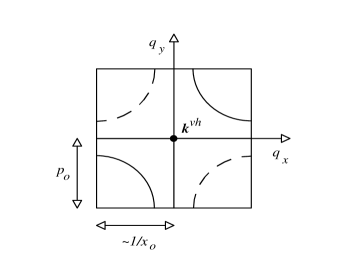
FIG. 1.: Constant energy contours of the quasiparticle dispersion near a 2D van Hove point ${\mathchoice{{\hbox{\boldmath$\displaystyle k$}}}{{\hbox{\boldmath$\textstyle k$}}}{{\hbox{\boldmath$\scriptstyle k$}}}{{\hbox{\boldmath$\scriptscriptstyle k$}}}^{vh}}$. $E({\mathchoice{{\hbox{\boldmath$\displaystyle k$}}}{{\hbox{\boldmath$\textstyle k$}}}{{\hbox{\boldmath$\scriptstyle k$}}}{{\hbox{\boldmath$\scriptscriptstyle k$}}}})-E^{vh}=q_{x}q_{y}$. The values of $\textstyle q$ are restricted to a region around the saddle point by the cutoffs $p_{o}$ and $x_{o}$.

Firstly, we evaluate the critical temperature at zero field when the vHs lies at the Fermi level. We need the ${\mathchoice{{\hbox{\boldmath$\displaystyle q$}}}{{\hbox{\boldmath$\textstyle q$}}}{{\hbox{\boldmath$\scriptstyle q$}}}{{\hbox{\boldmath$\scriptscriptstyle q$}}}}=0$ pair propagator (or pair susceptibility):[15]

$${\cal K}_{\beta}(0,0) = {\int_{x_{0}}^{\infty}dx\widetilde{K}_{\beta}(x,q_{y}=0)}$$ (9)

$$= {\int_{x_{o}}^{\infty}{dx\over x}\log\left[\tanh\left({x\pi\over{\beta_{c}p_{o}}}\right)\right]^{-1}}.$$ (10)

Here we have introduced a short distance cutoff $x_{0}$ in the x-direction.[16] At temperatures low compared with the bandwidth $x_{o}{\pi/{\beta p_{o}}}\ll 1$, the main contribution to the integral results from the small $x$ region and ${\cal K}_{\beta}(0,0)\sim 1/2\log^{2}\left[{x_{o}\pi}/{\beta p_{o}}\right]$. The zero field critical temperature is determined by the relation $1=g{\cal K}_{\beta_{c}}(0,0)$ and one recovers the standard result $T_{c}=\pi^{-1}x_{o}^{-1}p_{o}\exp(-\sqrt{2/g})$ compared to the weak coupling FL-BCS result $T_{c}\propto\exp(-1/\widetilde{g})$, where $\widetilde{g}\propto g$.

The pair propagator [Eq. (8)] can be evaluated in closed form at zero temperature and zero $\delta$. In this case, the gap equation [Eq. (3)] simplifies to

$$\widetilde{\Delta}(x)=g\int dx^{\prime}{1\over 2|x^{\prime}-x|}\log\left[{2p_{o}\over H|x^{\prime}+x|}\right]\widetilde{\Delta}(x^{\prime}),$$ (11)

with $|x^{\prime}-x|>x_{o}$. A lower bound for $H_{co}$ can be obtained by the variational method. A physically reasonable form for the gap function is $\widetilde{\Delta}(x)={1/\sqrt{2a}}\Theta(a-|x|)$, where $a$ is a length to be determined. The maximum eigenvalue is obtained for $a=e\sqrt{x_{o}p_{o}/2H}$ which leads to ${1/g}\gtrsim{1/4}\log^{2}\left({e^{2}p_{o}/2x_{o}H_{co}}\right).$ Thus $H_{co}\sim(e^{2}p_{o}/2x_{o})\exp(-2g^{-{1\over 2}})$. This implies

$${x_{o}H_{co}\over p_{o}}\sim\left({x_{o}T_{co}\over p_{o}}\right)^{\sqrt{2}}.$$ (12)

FIG. 2.: Variation of the $H_{c2}$ curve as a function of $\delta$, for $p_{o}/x_{0}=20$ and moderate coupling $g=0.2$, obtained by numerical lanczos solution of Eq. (3). Notice that $H_{co}$ has a much stronger dependence on $\delta$ that $T_{co}$. Upward curvature is observed in all curves down to a temperature of the order of $\delta$. For higher $\delta$, there is a small increase of $H_{c2}$ with temperature as the temperature averaged density of states increases.

This result should be contrasted with the usual FL-BCS scaling $H_{co}\sim T_{co}^{2}$. By expanding the kernel [Eq. (8)] around the zero temperature critical point, one can obtain the low temperature behavior of $H_{c2}$ and behaves as $H_{c}-H_{co}\sim-T\log{(H_{co}/T)}/\log{(x_{o}H_{co}/p_{o})}$. $H_{c}(T)$ does not saturate as $T$ goes to zero.

For temperatures close to the zero field critical temperature $T_{co}$, one can follow the Gorkov microscopic derivation of the Ginzburg-Landau equation to obtain

$$a\widetilde{\Delta}(x)+b(\partial^{2}_{x}-H^{2}x^{2})\widetilde{\Delta}(x)=0,$$ (13)

where

$$a = (T-T_{co}){d\over dT}\left[\int d^{2}{\mathchoice{{\hbox{\boldmath$\displaystyle r$}}}{{\hbox{\boldmath$\textstyle r$}}}{{\hbox{\boldmath$\scriptstyle r$}}}{{\hbox{\boldmath$\scriptscriptstyle r$}}}}K_{\beta}({\mathchoice{{\hbox{\boldmath$\displaystyle r$}}}{{\hbox{\boldmath$\textstyle r$}}}{{\hbox{\boldmath$\scriptstyle r$}}}{{\hbox{\boldmath$\scriptscriptstyle r$}}}})\right]_{T_{co}},$$ (14)

$$b = {1\over 2}\int d^{2}{\mathchoice{{\hbox{\boldmath$\displaystyle r$}}}{{\hbox{\boldmath$\textstyle r$}}}{{\hbox{\boldmath$\scriptstyle r$}}}{{\hbox{\boldmath$\scriptscriptstyle r$}}}}K_{\beta}({\mathchoice{{\hbox{\boldmath$\displaystyle r$}}}{{\hbox{\boldmath$\textstyle r$}}}{{\hbox{\boldmath$\scriptstyle r$}}}{{\hbox{\boldmath$\scriptscriptstyle r$}}}})x^{2}\cong{1\over 2}\int d^{2}{\mathchoice{{\hbox{\boldmath$\displaystyle r$}}}{{\hbox{\boldmath$\textstyle r$}}}{{\hbox{\boldmath$\scriptstyle r$}}}{{\hbox{\boldmath$\scriptscriptstyle r$}}}}K_{\beta}({\mathchoice{{\hbox{\boldmath$\displaystyle r$}}}{{\hbox{\boldmath$\textstyle r$}}}{{\hbox{\boldmath$\scriptstyle r$}}}{{\hbox{\boldmath$\scriptscriptstyle r$}}}})y^{2}.$$ (15)

Here, we have used the fact that $K_{\beta}({\mathchoice{{\hbox{\boldmath$\displaystyle r$}}}{{\hbox{\boldmath$\textstyle r$}}}{{\hbox{\boldmath$\scriptstyle r$}}}{{\hbox{\boldmath$\scriptscriptstyle r$}}}})$ is symmetric in the transformation $x\rightarrow y$. Setting $p_{o}\sim{1\over x_{o}}$, then $b_{x}\sim b_{y}$. For our van-Hove model with $\delta=0$, we have

$$a \sim {T_{co}-T\over T_{co}}\log\left[{p_{o}\over\pi x_{o}T_{co}}\right],$$ (16)

$$b \sim \left({p_{o}\over 2\pi T_{co}}\right)^{2},$$ (17)

$${dH_{c}\over dT} \sim -{x_{o}T_{co}\over p_{o}}\log\left[{p_{o}\over\pi x_{o}T_{co}}\right].$$ (18)

Note that for the 2D isotropic BCS superconductor, we would have $a\sim\rho(E_{F})(T_{c}-T)/T_{c}$. The vHs at the Fermi level is averaged out at a finite temperature $T_{co}$ and so, in the previous expressions, the density of states is replaced by an effective density of states $\log[\pi{x_{o}T_{co}/p_{o}}]$ giving a weak enhancement of the slope. Eqs. (12) and (18) show that there is an anomalous enhancement and consequently upward curvature of the upper critical field and that this upward curvature is strongly enhanced at weak coupling (low $T_{c}$). Thus in contrast to FL-BCS, normalized plots of ${H\over H_{co}}\left({T\over T_{co}}\right)$ do not fall on to a universal curve for different couplings.

To extend the above analysis to all temperatures and confirm the variational analysis requires a numerical approach. Discretizing in the $x$ direction, $x_{n}=n\epsilon$ where $n$ are integers, the integral gap equation becomes

$$\widetilde{\Delta}_{i}=g\sum_{ij}\widetilde{K}_{ij}\widetilde{\Delta}_{j}.$$ (19)

While the system is now discrete it remains infinite dimensional. However, the system can be truncated for finite $H$ because we need only consider solutions $\widetilde{\Delta}_{i}$ which are localized about the origin on a scale of the magnetic length.

The highest eigenvalue and corresponding gap function of Eq. (19) were obtained by the Lanczos method.

FIG. 3.: Gap functions $\widetilde{\Delta}(x)$ for two points of the $H_{c2}$ curve with $p_{o}/x_{0}=20$, $g=.2$ and $\delta=0$. One of the points is near the top of the $H_{c2}$ curve and the other near the bottom. Although the range of the gap functions is roughly the same (of the order of the magnetic length in each case), the functional forms of the two curves are different. For low $H_{c}/H_{co}$ we have the conventional behavior $\widetilde{\Delta}(x)\sim e^{-x^{2}H}$, while for $H_{c}/H_{co}\sim 1$, the gap function has an anomalously slow decay.

The results are displayed in Figs. 2 and 3. In Fig. 2, we have $H_{c2}$ curves for different values of $\delta$ and fixed coupling $g$. $H_{c2}$ saturates when $T<\delta$. When $\delta=0$, that is, when the Fermi energy coincides with the vHs, there is no saturation and the $H_{c2}$ curve shows an upward curvature through the complete temperature range in complete agreement with the variational calculation.

A qualitative understanding of these results is obtained as follows. In FL-BCS, the upper critical field is given by $1=g\rho(E_{F})\log(H+T^{2})$. In the vHs case, $\rho(E)$ is logarithmic divergent. Finite magnetic field or temperature smear out the density of states and $\rho(E_{F})$ should be replaced by $\log(H+T)$ at zero $\delta$. Thus $1\sim g\log(H+T)\log(H+T^{2})$. This leads to $H_{co}\sim T_{co}^{\sqrt{2}}$ as found above.

In conclusion, we have studied the suppression of the mean field superconducting instability of a clean weak coupling BCS superconductor in finite magnetic field at a 2D vHs. The upper critical field is strongly enhanced relative to $T_{c}$; this enhancement is described by the relation $H_{c2}(0)\sim T_{c}^{\sqrt{2}}$. The upper critical field falls linearly with temperature near $T=0$. These effects disappear rapidly when the Fermi level is tuned away from the Fermi level; more precisely, they are absent when $T_{c}<\delta$ defined above. The 2D vHs provides a simple example of a system where non-Fermi liquid normal state correlations show up strongly in the temperature dependence of the superconducting upper critical field.

RD would like to thank Junta Nacional de Investigação Científica e Tecnológica (Lisbon) for financial support.

REFERENCES

• [1] Also at: Cavendish Laboratory, Cambridge University, United Kingdom.
• [2] J. Labbe et al, Phys. Rev. Lett. 19, 1039 (1967).
• [3] J. E. Hirsch and D. J. Scalapino, Phys. Rev. Lett. 56, 2732 (1986).
• [4] J. Friedel,J. Phys. Condens. Matter 1, 7757 (1989); J. Labbe and J. Bok, Europhys. Lett. 3,1225 (1987).
• [5] C. C. Tsuei, D. M. Newns, C. C. Chi and P. C. Pattnaik, Phys. Rev. Lett. 65, 2724, (1990); D. M. Newns, C. C. Tsuei, P. J. M. van Bentum, P. C. Pattnaik and C. C. Chi, Phys. Rev. Lett. 73, 1695 (1994).
• [6] J. Friedel,J. Phys. (Paris) 48, 1787 (1987).
• [7] R. G. Dias and J. M. Wheatley, Phys. Rev. B 50,13887 (1994).
• [8] A. Sudbo, Phys. Rev. Lett. 74, 2575 (1995).
• [9] D. E. Prober et al, Phys. Rev. B 21, 2717 (1980);
• [10] A. P MacKenzie et al, Phys. Rev. Lett. 71, 1238 (1993); M. S. Osofsky et al, Phys. Rev. Lett. 71, 2315, (1993).
• [11] K. Murata et al, Synth. Met. A 341, 27 (1988).
• [12] L. P. Gorkov, JEPT 10, 593 (1960).
• [13] A. A. Abrikosov, L. P. Gorkov and I. E. Dzayloshinskii, Methods of Quantum Field Theory in Statistical Physics, p.323, Dover (1963).
• [14] There is some freedom in the choice of the phase term. An equivalent expression would be $\exp\{i[2{A}({r})]({r^{\prime}}-{r})\}$ and it would lead to the same results.
• [15] An equivalent expression is
$${\cal K}(0,0)={\int_{0}^{p_{o}}dp_{y}{1\over p_{y}}\log\left[{\tanh\left({\pi\over\beta}{x_{o}\over p_{y}}\right)}\right]^{-1}},$$
where the integrand is the 2D isotropic uniform pair propagator with Fermi velocity $v_{F}=p_{y}$.
• [16] It can be shown that $H_{c2}(T)$ depends only on the ratio $p_{o}/x_{o}$.