TPBU-95-6
Critical exponent of the localization length for the symplectic case

abstract

A new summability method was tested to calculate the critical exponent $\nu$ of the localization length for the symplectic case derived from the non-linear $\sigma$-model. Although we used the same series as Hikami and others, unlike them we were able to resum the series in two-dimensions (2D) and obtain the result $\nu\sim 1$. Values of $\nu$ in $2+\varepsilon$ dimensions seem to saturate the Harris inequality up to $\varepsilon=0.2$.

PACS numbers : 02.30.Lt, 71.30.+h, 72.15.Rn

(J. Phys. A: Math. Gen. 29, 289-294 (1996))

1. Introduction.- Anderson localization is known as a problem where the wave function localizes due to a random potential scattering [1]. The critical behaviour of the localization transition is described by the non-linear (NL) $\sigma$-model [2]. The NL$\sigma$-model explains succesfully various aspects of the Anderson localization, including the nonsingular density of states and three different universality classes - the orthogonal, unitary, and symplectic, depending on whether time-reversal symmetry is preserved or spin-flip scattering occurs.

The critical exponent $\nu$ describes the behaviour of the localization length $\lambda$ near the mobility edge $E_{c}$,

$$\lambda\sim(E_{c}-E)^{-\nu}.$$ (1)

To obtain critical exponents at the transition point in the framework of the NL$\sigma$-model, the scheme of the minimal subtraction by the dimensional regularization is usually used. The critical exponent $\nu$ of the correlation length or the localization length is then given by the relation

$$\nu=-\frac{1}{\beta^{\prime}(t_{c})},$$ (2)

where $t_{c}$ is the zero of the $\beta$ function and $\beta^{\prime}$ is t he derivative of $\beta$ with respect to $t$ [3]. In general, the $\beta$ function of the NL$\sigma$-model in $2+\varepsilon$ dimensions is given as

$$\beta(t)=\varepsilon\,t-\sum_{n=2}^{\infty}a_{n}t^{n},$$ (3)

where the coefficients $a_{n}{}^{\prime}s$ do not depend on $\varepsilon$ and $a_{2}\neq 0$ [4]. In the symplectic case, which is the universality class corresponding to time-reversal symmetry and strong spin-orbit coupling, the $\beta$ function to five-loop order is given by

$$\beta_{so}(t)=\varepsilon\,t+t^{2}-\frac{3}{4}\zeta(3)\,t^{5}-\frac{27}{64}\zeta(4)\,t^{6}+{\cal O}(t^{7}),$$ (4)

where $\zeta$ is the Riemann $\zeta$-function [4].

2. Methods.- To extract the critical exponent $\nu$, only the Borel-Padé method has been used so far [4]. The Borel summability method, when applied to the series of the form (3), consists in the following transformation,

$$\sum_{n=1}^{\infty}a_{n}t^{n}\longrightarrow\frac{1}{t}\int_{0}^{\infty}e^{-u/t}\sum_{n=1}^{\infty}a_{n}\frac{u^{n}}{n!}\,du.$$ (5)

For finite series, relation (5) is useless since it is an identity. One can integrate term by term, by using

$$\frac{1}{t}\int_{0}^{\infty}e^{-u/t}u^{n}du=n!\,t^{n}.$$

However, for infinite series the second form in (5) may have a much wider range of applicability. For example, in the case of the series $\sum_{n=0}^{\infty}z^{n}$ the second form converges in the whole complex halfplane Re $z<1$ despite that the original series being divergent for $|z|>1$, outside its radius of convergence. Having only a finite number of a series up to order $N$ at one’s disposal, such as in the present case, the integrand in (5) can be approximated by the Padé approximation which generates an infinite power series coinciding up to order $N$ with the original series. The resulting method is called the Borel-Padé method.

Figure 1: a) The actual region of convergence for the Borel method in the case of the Taylor series of an analytic function $f(z)$ is a polygon which is obtained by removing half-planes from the complex plane which lie behind a perpendicular to the ray from the origin passing through the singularity (a cross). b) In the case of our method, the actual region of convergence is obtained by only removing the part of the ray behind each singularity. Such region is called the Mittage-Leffler star.

Several years ago we have developed a method [5] which consists in a similar transformation as (5) but with $e^{-u/t}$ replaced by $e^{-e^{u/t}}$ and $n!$ replaced by

$$\mu(n)=\int_{0}^{\infty}e^{-e^{u}}u^{n}\,du.$$ (6)

Moments $\mu(n)$ are increasing more slowly then $n!$ (they behave roughly as $\ln^{n}(n)$ when $n\rightarrow\infty$), but as far as analytic properties are concerned this results in a wider region of convergence. If $f(z)$ denotes an analytic continuation of a power series with a non-zero radius of convergence, then our method gives a finite result $f(z)$ in the so-called Mittag-Leffler star of $f(z)$ [5]. In the case of the series $\sum_{n=0}^{\infty}z^{n}$ it means that our method converges in the whole complex plane except for the interval $[1,\infty)$. For a general power series, the Mittag-Leffler star is obtained in the following way (see Fig. 1). First, one draws rays from the origin and passing through singularities of $f(z)$. The Mittage-Leffler star is the region which remains in the complex plane after the part of the ray beyond each singularity is removed. We recall that the actual region of convergence for the Borel method is a polygon which is obtained by removing half-planes from the complex plane which lie behind a perpendicular to the ray from the origin passing through the singularity (see Fig. 1). If one has only a finite number of terms of a series at disposal, one can use the Padé approximation of the integrand in (5) in the same way as when the Borel method is used. We shall call the resulting method the $\mu$-Padé method. Both, the Borel method and our method are so-called analytic moment-constant summability methods [5, 6]. They can be applied to both convergent and divergent series.

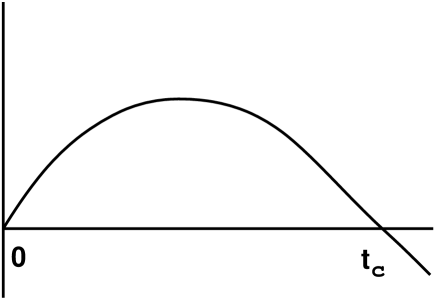
Figure 2: Typical behaviour of the $\beta$ function for the symplectic case after it has been resummed by the diagonal $\mu$-Padé method.

3. Results.- One of the motivations in using the $\mu$-Padé method for the symplectic case was the fact the series (4) is not Borel summable and the Borel-Padé method does not work for this case [4]. In the $2D$ symplectic case, to leading order, so-called weak anti-localization occurs [7] and until recently it appeared that this result remain unchanged by higher order terms. This included the strange result that there is no fixed point (and hence no transition and no localization) for the $2D$ symplectic case [8]. We have applied the diagonal [3/3] $\mu$-Padé method directly to the $\beta_{so}(t)$ and looked for its zero $t_{c}(\varepsilon)$ as a function of $\varepsilon$ (see Fig. 2). By using relation (2) we have found that as $\varepsilon\downarrow 0$, the critical exponents

$$\nu\rightarrow 0.98$$ (7)

in the $2D$ symplectic case. The $\beta$ function for the orthogonal universality class is related to $\beta$ function for the symplectic universality class by substituting $t$ in Eq. (4) by $-2t$ [4]. Therefore, because the diagonal [3/3] $\mu$-Padé method works for the symplectic case, it cannot be applied to the orthogonal case, since the Padé approximant, having a polynomial of order $3$ in the denominator, develops a pole in the integration interval. A similar statement applies to the diagonal [3/3] Borel-Padé method, which, in contrast, works for the orthogonal case and therefore does not for the symplectic case [4].

In the following, we have scanned the $\varepsilon$-expansion by varying $\varepsilon=d-2$, where $d$ is the space dimension, within the interval $\varepsilon\in(0,1]$. Results are presented in Table I.

TABLE I. $\beta^{\prime}(t_{c})$ and the critical coefficient $\nu$ as a function of $\varepsilon$

$\varepsilon$	0.1	0.2	0.3	0.4	0.5	0.6	0.7	0.8	0.9	1.0
$\beta^{\prime}(t_{c})$	-1.05	-1.14	-1.27	-1.47	-1.74	-2.1	-2.58	-3.2		-0.50
$\nu$	0.95	0.88	0.79	0.68	0.57	0.48	0.39	0.31		2

4. Discussion.- We have checked whether our results satisfy the Harris inequality [9],

$$\nu\geq\frac{2}{d},$$ (8)

derived under the assumption of the validity of one-parameter scaling. Up to an error due to the finite number of terms for $\beta_{so}(t)$ [see (4)], our result seems to saturate the inequality (8) up to $\varepsilon=0.2$. As $\varepsilon$ increases further, $\nu$ ceases to satisfy (8) and eventually around $\varepsilon=0.9$ the diagonal $\mu$-Padé method collapses. The reason is that the Padé approximant develops a pole on the integration interval. For $\varepsilon=1$, the $\mu$-Padé method starts to work again and our result

$$\nu=2$$ (9)

satisfies inequality (8). However, because of the collapse of the diagonal $\mu$-Padé method at $\varepsilon=0.9$, this result must be taken with some reservations. Since the $\epsilon$ expansion (3) is an asymptotic expansion, it is difficult to make an extrapolation too far away from the limiting point ($D=2$ in our case), given that the extrapolation is based on incomplete knowledge of the $\beta$ function. Nevertheless, it provides a substational improvement over previous analytical results, and there is always a chance that further terms of the $\beta$ function will make our results better. It is worthwhile to mention that the actual convergence or divergence of an asymptotic series is not as important for applicability of an analytic summability method as whether asymptotic series obey the strong asymptotic conditions (SAC) [5, 10]. The latter ensure that there exists only one function with the required analytic properties and a given asymptotic expansion. For example, given a convergent asymptotic series $\sum_{0}^{\infty}z^{n}$ in the right complex half plane, without the validity of the SAC the sum of this series can be any function of the form $1/(1-z)+As^{B}e^{-C/z}$ with $A$, $B$, and $C>0$ arbitrary constants.

In the $2D$ symplectic case, our result (7) for the critical exponent $\nu$ is smaller than $\nu\sim 2.5$ [11] or $\nu\sim 2.74$ [12] obtained by numerical scaling analysis using, respectively, the Evangelou-Ziman model [13] or Ando’s model [14]. A similar disagreement between field theory predictions and tight-binding scaling methods is also known to exist for the $3D$ orthogonal case, where the former yields $\nu\sim 1$ and the latter $\nu\sim 1.4$. It is interesting to note that a disagreement also exists for the results for the critical exponent $\nu$ obtained by the numerical scaling analysis and that obtained by the best fit to the critical level distribution $P(s)$ in the $2D$ symplectic case at the mobility edge [15],

$$P(s)=Bs^{4}\exp\left(-As^{\gamma}\right).$$ (10)

Here parameter $\gamma$ is given by

$$\gamma=1-\frac{1}{\nu^{*}d},$$ (11)

$d$ is the dimensionality of the system, $A$ is a numerical factor which depends on the dimensionality, and $B$ is to be found from the normalization conditions [15]. The critical exponent $\nu^{*}$ in (11) should be identical to $\nu$. However recent numerical analysis implies that $\nu^{*}=0.7\pm 0.08$ [16] or $\nu^{*}\sim 0.77$ [17] for Ando’s model [14], and $\nu^{*}=0.83\pm 0.7$ [11] for the Evangelou-Ziman model [13]. A comparison with (8) shows that $\nu^{*}$ even violates the Harris inequality [9] [however $\nu^{*}$ satisfies a weaker relation, $\nu^{*}>1/d$, which suffices to derive (10)]. Surprisingly enough, our result (7) for the critical exponent $\nu$ in the $2D$ symplectic case for the localization length is actually very close to $\nu^{*}$ and it seems to be tempting to say that the critical exponent obtained from the NL$\sigma$ is just $\nu^{*}$. That, however, would be premature, because in the $3D$ orthogonal case the overall behaviour of $P(s)$ has been claimed to be well fitted with $\nu$ obtained from the numerical scaling analysis [18].

To conclude, we have demonstrated that the $\mu$-Padé method can be useful in determining critical exponents. In principle, our method can be used as an alternative to the Borel-Padé summability method, whenever a result is obtained in a form of a power (asymptotic) series, such as in the case of high temperature expansion, weak coupling expansion, etc. In connection with disordered systems, it would be interesting to use our method for a calculation of the density of states and the diffusion constant for the problem of an electron moving in two dimensions in the lowest Landau level and in a random potential, which has been analyzed by the Borel-Padé method [19]. It was suggested that our summability method be used for the location of critical points [10], since it finds singularities of an analytic function much more precisely than the Borel method (cf. Fig. 1). An application of the $\mu$-Padé method to other problems will be given elsewhere.

I should like to thank I. V. Lerner for discussion and suggestions on the literature and M. W. Long for his help with computer facilities. I should also like to thank referees for useful suggestions. This work was supported by EPSRC grant number GR/J35214. Partial support by the Grant Agency of the Czech Republic under Project No. 202/93/0689 is also gratefully acknowledged.

References

- [1] Anderson P W 1958 Phys. Rev. 109 1492
-
[2]
Wegner F 1979 Z. Phys. B 35 207
Hikami S 1981 Phys. Rev. B 24 2671 - [3] Brézin E and Zinn-Justin J 1976 Phys. Rev. B 14 3110
- [4] Hikami S 1992 Prog. Theor. Phys. 107 Suppl. 213
- [5] Moroz A 1990 Czech. J. Phys. B 40 705; 1990 Commun. Math. Phys. 133 369; 1991 PhD thesis, Prague Institute of Physics (compuscript without figures available in the hep-th network as hep-th/9206074).
- [6] Hardy G 1949 Divergent series (Oxford: Oxford Univ. Press)
- [7] Oppermann R and Jüngling K 1980 Phys. Lett. 76A 449
- [8] Kramer B and MacKinnon A 1993 Rep. Prog. Phys. 56 1469
-
[9]
Harris A B 1974 J. Phys. C: Solid State Phys.
7 1671
Chayes J T, Chayes L, Fisher D S and Spencer T 1986 Phys. Rev. Lett. 57 2999
See also Kramer B 1993 Phys. Rev. B 47 9888 - [10] Moroz A 1992 Czech. J. Phys. B 42 753
- [11] Evangelou S N 1995 Phys. Rev. Lett. 75 2550
- [12] Fastenrath U et al. 1991 Physica A 172 302
- [13] Evangelou S N and Ziman T 1987 J. Phys. C: Solid State Phys. 20 L235
- [14] Ando T 1989 Phys. Rev. B 40 5325
- [15] Aronov A G, Kravtsov V E, and Lerner I V 1994 JETP Lett. 59 39
- [16] Schweitzer L and Zharakeshev I Kh 1995 J. Phys.: Cond. Matt. 7 L377
- [17] Ohtsuki T and Ono Y (cond-mat/9509146)
-
[18]
Evangelou S N 1994 Phys. Rev. B 49 16 805
Hofstetter E and Schreiber M 1994 Phys. Rev. B 49 14 726 -
[19]
Hikami S 1984 Phys. Rev. B 29 3726
Singh R R P and Chakravarty S 1985 Nucl. Phys. B265 265