cond-mat/9507xxx
Roughness of randomly crumpled elastic sheets

Abstract

We study the roughness of randomly crumpled elastic sheets. Based on analytical and numerical calculations, we find that they are self affine with a roughness exponent equal to one. Such crumpling occurs e.g. when wet paper dries. We also discuss the case of correlated crumpling, which occurs in connection with flattening of randomly folded paper.

Take a sheet of paper. Wet it with water and let it dry. The sheet will crumple. A closer look at the dried surface does not reveal any preferred length scale in the crumpling. Rather, smaller crumples appear inside the larger ones, and so on to smaller and smaller scales, finally to reach the scale of the fibers making up the paper. Surfaces having this appearance are in fact abundant in nature. For example, fracture surfaces show roughness on all scales, as do surfaces that have been corroded [1, 2, 3, 4]. Recently, mathematical tools have been developed to describe such surfaces in terms of their scaling properties [5, 6]. We will in this letter analyse the roughness of dried paper surfaces in light of these scaling properties based on a theoretical model originating from the theory of linear elasticity of thin plates [7, 8]. We also note the connection between this problem and the problem of unfolding a randomly wrapped paper [9]: Wrap a sheet of paper randomly into a tight ball. Then unfold it and try to flatten it as much as possible. It will stay rough by much the same mechanism that makes dried paper rough. However, the foldings of the paper have introduced long-range correlations between the local crumpling of the paper. These long-range correlations may change the roughness of the sheets. Experimental measurements of this roughness show, however, that it is within the experimental uncertainty equal to the roughness due to uncorrelated crumpling. We generalize the one-dimensional model of reference [9] to a two-dimensional elastic sheet. However, the roughness found in this model is larger than the one found in the random crumpling case and in the experiments.

The scaling properties alluded to above, are more precisely described through the concept of self affinity. We choose for a given surface the $(x,y)$ plane to be the mean plane, and the $z$ axis to be the normal direction. The surface is self affine if it is (statistically) invariant under the rescaling transformation

$$\cases{x&$\to\lambda x$\cr y&$\to\lambda y$\cr z&$\to\mu(\lambda)z\;,$\cr}$$ (1)

where $\lambda$ is a arbitrary scaling factor, and $\mu$ is a function of $\lambda$. Group properties on the transformation (1) imply that $\mu$ is a homogeneous function of $\lambda$ characterized by an exponent $H$, $\mu\propto\lambda^{H}$. This exponent is the roughness index. The aim of this letter is to determine the roughness index of a randomly crumpled elastic sheet.

We return to the problem of wetting and then drying paper. By pouring water on one side of a sheet of paper, it immediately curls up away from the wetted side. This is due to the paper expanding locally on the wetted side. If, however, the paper is wetted on both sides, a uniform expansion occurs, and the now thoroughly wet paper will stay flat. However, as it begins to dry, it roughens. There are two mechanisms behind this roughening: (1) internal torques which bend the surface locally due to inhomogeneous contractions in the perpendicular direction of the sheet, which in turn are due to inhomogeneities in the structure of the paper itself and/or differences in the drying drying rates from the two sides of the paper, and (2) buckling due to locally homogenous in-plane contractions of the paper. In deciding which of these two mechanisms is the dominant one, we note that buckling, which is a non-linear elastic problem, produce multiple stable bending modes, while the first process to a first approximation is a linear problem producing unique bending modes. Using whether a unique roughened shape of the paper results when the paper has dried, or there are several equivalent ones, we find that mostly the former is the case. We thus conclude that it is the internal torques which dominate.

When wrapped paper is flattened, the resulting roughness is caused by internal torques and not buckling.

In light of the above discussion, we base our modeling on the linearized equation for flexion of an elastic plate under a loading $q(x,y)$ in the $z$ direction:

$$D\Delta\Delta\zeta=q\;,$$ (2)

where $D$ is the flexural rigidity of the plate, (chosen to be unity, $D=1$, in the following), and $\zeta(\vec{x})$ is the vertical deflection of the plate at $\vec{x}=(x,y)$ [8]. Equation (2) is known as the Germain equation. However, the forces acting on the surface in the case of drying paper are not external. We are rather seeking a behavior where locally the surface at $\vec{x}$ would adopt a non-zero curvature $\Delta\zeta=\eta(\vec{x})$ if it were isolated from its neighborhood. The $\eta(\vec{x})$ is chosen here to be a random field. This noise term is assumed to represent the fluctuations in curvature due to the local inhomgeneous contractions of the paper. However, $\Delta\zeta$ is not a force, $\Delta\Delta\zeta$ is, see equation (2). Therefore, the equation that balances the forces locally in the plane is

$$\Delta\Delta\zeta=\Delta\eta\;.$$ (3)

With the assumption that $\eta(\vec{x})$ is an uncorrelated random field, we have that $\langle\eta(\vec{x}_{1})\eta(\vec{x}_{2})\rangle=c^{2}\delta(\vec{x}_{1}-\vec{x}_{2})$, where $\langle\dots\rangle$ signify ensemble average, and $\delta(\vec{x})$ is the Dirac distribution. Note, however, that modeling the unfolded and flattened paper, the stochastic field $\eta$ has long range correlations build into it stemming from the folding process.

Let us assume a system of size $L\times L$ where $L$ is large. The height fluctuations, $\langle(\zeta(\vec{x}_{1})-\zeta(\vec{x}_{2}))^{2}\rangle$, may easily be calculated by using Green’s method. We have that

$$\zeta(\vec{x})=\int d\vec{y}\>G(\vec{x}-\vec{y})\Delta_{y}\eta(\vec{y})=\int d\vec{y}\>\Delta_{x}G(\vec{x}-\vec{y})\eta(\vec{y})\;,$$ (4)

where $G(\vec{x})$ is the solution of $\Delta\Delta\zeta=\delta(\vec{x})$, which in Fourier space is $\tilde{G}(\vec{k})=1/k^{4}$. Thus, we have that

$$\langle\zeta(\vec{x}_{1})\zeta(\vec{x}_{2})\rangle = \int\int d\vec{y}_{1}d\vec{y}_{2}\>\Delta_{x_{1}}G(\vec{x}_{1}-\vec{y}_{1})\Delta_{x_{2}}G(\vec{x}_{2}-\vec{y}_{2})\langle\eta(\vec{y}_{1})\eta(\vec{y}_{2})\rangle$$ (5)

$$= c^{2}\int k^{4}\>d\vec{k}\>\tilde{G}(\vec{k})\tilde{G}(-\vec{k})e^{i(\vec{x}_{1}-\vec{x}_{2})\cdot\vec{k}}=c^{2}\int{{d\vec{k}}\over{k^{4}}}e^{i(\vec{x}_{1}-\vec{x}_{2})\cdot\vec{k}}\;.$$ (6)

We may now calculate the height fluctuations:

$$\langle(\zeta(\vec{x}_{1})-\zeta(\vec{x}_{2}))^{2}\rangle=2c^{2}\int_{0}^{2\pi}d\phi\>\int_{1/L}^{\infty}{{dk}\over{k^{3}}}\>\left(1-e^{i|\vec{x}_{1}-\vec{x}_{2}|k\cos(\phi)}\right)=CL|\vec{x}_{1}-\vec{x}_{2}|^{2}\;,$$ (7)

where $C$ is a constant. This last result shows that the roughness index is

$$H=1\;.$$ (8)

One should also note that the variance of the height scales as

$$\langle\zeta^{2}(\vec{x})\rangle\propto c^{2}L^{2}$$ (9)

with the system size. The square dependence on $L$ is also a reflection of $H=1$.

A direct way to model numerically surfaces following equation (3), is to integrate this equation to get

$$\Delta\zeta=\eta+\phi\;,$$ (10)

where $\phi$ is a solution of the equation $\Delta\phi=0$. We now assume that our system of size $L\times L$ has biperiodic boundary conditions. Then, we have that $\langle\Delta\zeta\rangle=0$ if the field $\zeta$ is to be continuous. Equation (10) then leads to the condition $\langle\phi\rangle=-\langle\eta\rangle$ on $\phi$. The solution of the Laplace equation with biperiodic boundary conditions is a constant, $\phi=constant=-\langle\eta\rangle$. Thus, we have in Fourier space that

$$\tilde{\zeta}={1\over k^{2}}\left(\tilde{\eta}-\langle\eta\rangle\right)\;.$$ (11)

This is straight forward to implement on the computer.

In addition to generating the solution of equation (3) through equation (11), we have discretized (3) and solved it through an iterative method. This method raises principal questions in that the noise term $\eta$ is not a smooth function, but varies rapidly on all scales, including the one chosen as our lattice constant in the discretization. This is a typical problem faced when modeling strongly disordered systems. However, we note that a priori a continuum description of a strongly disordered system (where this is at all possible) is not more fundamental than a description based on a discrete system.

The discretization we have chosen is the following one: We use a triangular tiling of rhombical plaquettes as shown in figure 1 [11]. The flexural energy associated with plaquette $0394$ (the numbering refers to the nodes of figure 1) is $\epsilon_{0394}=(\zeta_{0}-\zeta_{3}+\zeta_{9}-\zeta_{4}+\eta_{34})^{2}$, where $\eta_{34}$ corresponds to the noise $\eta$ of equation (3). Each elementary triangle is covered by three plaquettes, e.g. triangle $034$ is the intersection of plaquettes $0394$, $0345$ and $0234$. With this construction, the dependence of the elastic energy of the network on a given node 0 in figure 1 is given by the sum

$$\epsilon_{0} = (\zeta_{0}-\zeta_{1}+\zeta_{7}-\zeta_{2}-\eta_{12})^{2}+(\zeta_{0}-\zeta_{2}+\zeta_{8}-\zeta_{3}-\eta_{23})^{2}$$ (12)

$$+ (\zeta_{0}-\zeta_{3}+\zeta_{9}-\zeta_{4}-\eta_{34})^{2}+(\zeta_{0}-\zeta_{4}+\zeta_{A}-\zeta_{5}-\eta_{45})^{2}$$ (13)

$$+ (\zeta_{0}-\zeta_{5}+\zeta_{B}-\zeta_{6}-\eta_{56})^{2}+(\zeta_{0}-\zeta_{6}+\zeta_{C}-\zeta_{1}-\eta_{61})^{2}$$ (14)

$$+ (\zeta_{0}-\zeta_{1}+\zeta_{2}-\zeta_{3}+\eta_{02})^{2}+(\zeta_{0}-\zeta_{2}+\zeta_{3}-\zeta_{4}+\eta_{03})^{2}$$ (15)

$$+ (\zeta_{0}-\zeta_{3}+\zeta_{4}-\zeta_{5}+\eta_{04})^{2}+(\zeta_{0}-\zeta_{4}+\zeta_{5}-\zeta_{6}+\eta_{05})^{2}$$ (16)

$$+ (\zeta_{0}-\zeta_{5}+\zeta_{6}-\zeta_{1}+\eta_{06})^{2}+(\zeta_{0}-\zeta_{6}+\zeta_{1}-\zeta_{2}+\eta_{01})^{2}\;.$$ (17)

The total elastic energy of the network is the sum $E=\sum_{i=1}^{N}\epsilon_{i}/12$, where $i$ runs over all $N$ nodes. In the limit of a vanishing lattice constant, $\delta$, $\partial\epsilon_{0}/\partial\zeta_{0}=0$ leads to the equation

$$\delta^{4}\Delta\Delta\zeta={{\delta^{2}}\over{12}}\Delta\eta+{{4\delta^{4}}\over 3}\Delta\Delta\eta+\dots\;.$$ (18)

When $\eta$ is a smooth function in the scale of $\delta$, the second term on the right hand side of equation (18) is small compared to the first term. However, if $\eta$ is not smooth, it will be of the same order as $\Delta\sim 1/\delta^{2}$, and the second term (and those we have not explicitly written in (18)) will be of the same size as the first. This is the case we deal with here. However, even though the implementation (12) does not reproduce (3) on small scale when $\eta$ is not smooth, the large scale features will be the same as predicted by the continuum equations. Had our basic equations not been linear, however, such a conclusion could not have been drawn. We note, furthermore, that equation (12) is an equally accurate but distinct modelization of the original problem, as the one based on the continuum theory, (3).

The noise term $\eta_{ij}$ in (12) is associated with the bond $ij$, which in turn is associated with a plaquette. We choose the value of $\eta_{ij}$ to be either 1 or $-1$ with equal probability. We implement biperiodic boundary conditions. For a given distribution of noise terms $\eta_{ij}$, we minimize the total energy $E$ using a conjugate gradient algorithm as described in [12]. In figure 2, we show a typical crumpled surface of size $L\times L=256\times 256$.

In order to measure the roughness index we generated an ensemble consisting of 1000 networks of size $L=10$, 1000 samples of size $L=20$, 800 samples of size $L=30$, 600 samples of size $L=40$, 200 samples of size $60$, 80 samples of size $L=80$, 40 samples of size $L=100$, 20 samples of size $L=150$, and 10 samples of size $L=200$. For each sample we measured the width defined as $w^{2}=(\sum_{i}\zeta_{i}^{2})/N-(\sum_{i}\zeta_{i})^{2}/N^{2}$, which corresponds to (9), and then averaged this quantity over all samples with the same size $L$. The result is shown in figure 3. We find that $w\propto L^{H}$ with $H=1.0\pm 0.05$, in agreement with the predicted $H=1$. In figure 4 we show the power spectrum $P(k)$, which is the Fourier transform of the height-height correlation function, measured along one-dimensional profiles and averaged over 10 samples of size $256\times 256$. $k$ is the wave number. For a self-affine surface, one expects $P(k)\propto k^{-(1+2H)}$. We find a slope equal to $-3.0\pm 0.1$ in figure 4, again consistent with a roughness index equal to one.

Thus, we have succeded in demonstrating how a simple linear elastic theory of crumpled surfaces can generate non-trivial self-affine surfaces. It would be very interesting to see how these theoretical results match with experiments. We furthermore note that we may use these results to generate large self-affine surfaces by e.g. spotwise random heating of elastic plates.

We now turn to the problem of randomly folded paper. The folding process induces in the paper a bending along the fold line somewhat similar to that observed when wet paper dries. Suppose now we fold the paper a first time. This produces a straight bend. However, the next fold — when the paper is unwrapped again — will change direction when it meets the first fold, unless this second folding is perpendicular to the first one. In addition, the bending of the second fold will change “sign” when it crosses the first fold. Thus, taking as starting point the one dimensional geometrical model introduced in reference [9], we implement the following two-dimensional model. We associate with each plaquette in a square lattice of size $2^{N}\times 2^{N}$ a value $\eta$. Assign to the line of plaquettes with coordinates $(2^{(}N-1),j)$, where $j=1$, … $2^{N}$, equal values for $\eta$, either $+1$ or $-1$. Then, go to line $(i,2^{N-1})$, where $i=1$, …, $2^{N-1}$. Assign to the first node an $\eta$-value equal to either $+1$ or $-1$ with equal probability. This value is reproduced for all subsequent nodes along this line until the previous line is encountered at $(i=2^{N-1},2^{N-1})$. Then, for all $(i>2^{N-1},2^{N-1})$, we assign the opposite value for $\eta$. We then go to the line $(2^{N-2},j)$, choose an $\eta$-value equal to $\pm 1$ for node $(2^{N-2},1)$, reproduce this value until we cross an older line, and then change sign for the subsequent $\eta$ values. Each time an older line is met, we change sign in the assigning of $\eta$ values. This construction is repeated over and over until all nodes has a value for $\eta$ associated with it. We show in figure 5 a pattern of bending lines produced this way for a $64\times 64$ lattice. Black line means an associated $\eta=1$, and gray means that the associated $\eta=-1$.

We then proceed to solve equation (3) with this distribution of $\eta$ values. In practice, we used the solution given in equation (11). We show in figure 6 a $256\times 256$ sheet produced this way. We note the similarity with figure 2 that was generated from a random distribution of $\eta$ values. However, an analysis of the power spectrum of an ensemble of such lattices (20 samples of size $256\times 256$) gave the result shown in figure 7, where we plot on log-log scale $P(k)$ vs. $k$ in the same way as in figure 4. There is a rich structure in this power spectrum which reflects the correlations induced by the folding process. Attempting to extract a power law from this structure, we show astraight line that follows the densest region of the plot. This curve has a slope of $-4$, thus indicating a roughness index equal to $1.5\pm 0.1$ (from $1+2H=4$). This is appreciably larger than what was found for the randomly crumpled paper, $H=1$, and the experimental study of the randomly folded paper [9]: $Hi\approx 0.9$.

We have, thus, shown in this letter how a random internal bending process of an elastic plate leads to a self affine structure with roughness index equal to one. Such processes are met e.g. when wet paper dries. We have also studied the case of a correlated bending process, i.e. when paper is crumpled into a tight ball and then unfolded and flattened. We find through a simple model for the correlations a roughness index which is higher than the one found in the random crumpling case.

F.T. thanks Lafarge-Coppée and the CNRS through the Groupement de Recherche Milieux Hétérogènes Complexes for financial support. A.H. thanks the ESPCI for a visiting professorship during which tenure this work was done. Further support came from the CNRS and the NFR through a Programme Internationale de Coopération Scientifique.

FIG. 1.: The numerical calculation is done using a triangular tiling of rhombical elastic plaquettes as shown in this figure.

FIG. 2.: A randomly crumpled sheet of size $256\times 256$.

FIG. 3.: Average width $w$ of sheets of size $L\times L$. The slope of the broken line is 1.0.

FIG. 4.: Power spectrum $P(k)$ as a function of wave number $k$ measured along one-dimensional profiles of surfaces that have been randomly crumpled. The curve is an average over all 256 profiles of each of 10 samples of size $256\times 256$. The slope of the broken line is $-3.0$.

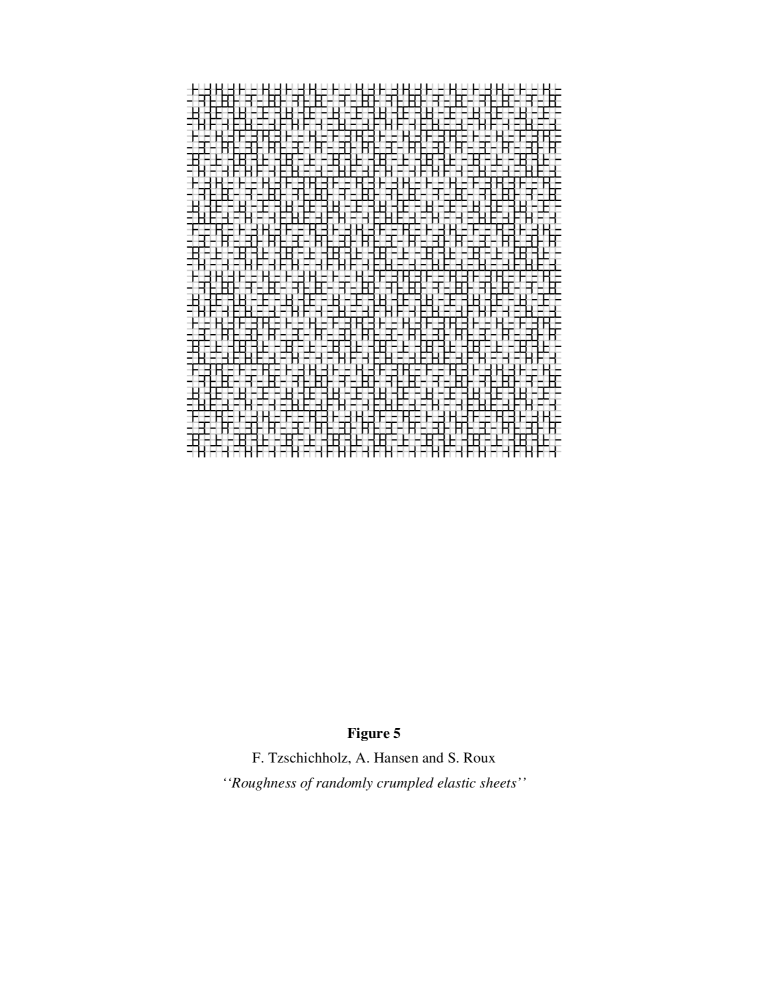
FIG. 5.: A folding pattern generated by the algorithm described in the text. Black line means the bend is “upwards” while a gray line means that the bend is “downwards.” The size here is $64\times 64$.

FIG. 6.: A sheet that has been been crumpled through the random folding algorithm. The size is $256\times 256$.

FIG. 7.: Power spectrum $P(k)$ as a function of wave number $k$ for the randomly folded surfaces. We measured along one-dimensional profiles over 20 samples of size $256\times 256$. The slope of the broken line is $-4.0$.

REFERENCES

- [1] F. Family and T. Vicsek, Dynamics of fractal surfaces (World Sci. Publ., Singapore, 1991).
- [2] P. Meakin, Phys. Rep. 235, 189 (1993).
- [3] T. Halpin-Healy and Y.C. Zhang, Phys. Rep. 254, 215 (1994).
- [4] A.L. Barabási and H.E. Stanley, Fractal concepts in surface growth (Cambridge University Press, Cambridge, 1995).
- [5] B.B. Mandelbrot, The fractal geometry of nature (W.H. Freeman, San Fransisco, 1982).
- [6] J. Feder, Fractals (Academic Press, New York 1988).
- [7] A. E. H. Love, A treatise on the mathematical theory of elasticity (Dover, New York, 1944).
- [8] M. Filonenko-Borodich, Theory of elasticity (Dover, New York, 1965).
- [9] F. Plouraboué and S. Roux, Roughness of randomly crumpled surfaces: Experimental study preprint, 1995.
- [10] S.P. Timoshenko, History of Strength of Materials (McGraw-Hill, New York, 1953).
- [11] S. Roux and A. Hansen, J. Phys. A 21, L941 (1988).
- [12] G.G. Batrouni and A. Hansen, J. Stat. Phys. 52, 747 (1988).