Off-equilibrium dynamics in finite dimensional spin glass models

Abstract

The low temperature dynamics of the two- and three-dimensional Ising spin glass model with Gaussian couplings is investigated via extensive Monte Carlo simulations. We find an algebraic decay of the remanent magnetization. For the autocorrelation function $C(t,t_{w})=[\langle S_{i}(t+t_{w})S_{i}(t_{w})\rangle]_{av}$ a typical aging scenario with a $t/t_{w}$ scaling is established. Investigating spatial correlations we find an algebraic growth law $\xi(t_{w})\sim t_{w}^{\alpha(T)}$ of the average domain size. The spatial correlation function $G(r,t_{w})=[\langle S_{i}(t_{w})S_{i+r}(t_{w})\rangle^{2}]_{av}$ scales with $r/\xi(t_{w})$. The sensitivity of the correlations in the spin glass phase with respect to temperature changes is examined by calculating a time dependent overlap length. In the two dimensional model we examine domain growth with a new method: First we determine the exact ground states of the various samples (of system sizes up to $100\times 100$) and then we calculate the correlations between this state and the states generated during a Monte Carlo simulation.

I Introduction

In spin glasses [1] below the transition temperature characteristic non-equilibrium phenomena can be observed [2]. The typical experiment where these phenomena are encountered is the measurement of the (thermo-)remanent magnetization. The procedure is the following: A spin glass sample is rapidly cooled within a magnetic field to a temperature below the transition temperature $T_{g}$ and then the field is switched off after a certain waiting time $t_{w}$. The striking observation then is that the decay of the magnetization $M(t)$ is found to depend on the waiting time $t_{w}$ even on laboratory time scales, a phenomenon called aging [3]. Aging is not restricted to spin glasses and has also been found in other disordered or amorphous systems such as polymers [4], high temperature superconductors [5] and charge-density wave systems [6] where certain quantities show a characteristic history dependence.

Several attempts have been made to explain this behavior theoretically. However, it has not been possible up to now to determine the non-equilibrium dynamics of short-range, finite-dimensional spin glass models starting from a microscopic Hamiltonian analytically. Thus one depends on phenomenological models which are either of a hierarchical type where the relaxation process is described by diffusion in a tree like structure of phase-space [7, 8] or scaling theories which consider the energetically low lying excitations in real space which are supposed to be connected cluster of reversed spins [9, 10]. An important ingredience of the latter theories are domain growth laws which determine the growth of the average domain size in dependence of the waiting time. Experimentally this quantity cannot be measured whereas in Monte Carlo (MC) Simulations one has direct access to all quantities of interest. Thus MC Simulations are an important touchstone for phenomenological theories and their underlying assumptions.

In this paper we present the results of large scale MC simulations of the two (2D)- and three-dimensional (3D) Ising spin glass model with nearest neighbour interactions and a continuous bond distribution. The focus is on the three dimensional model whose low-temperature dynamics is examined in detail by calculating correlation functions in time and space. In earlier works [11, 12] mainly the case of a binary bond distribution was studied and the focus was on the time-dependent auto- correlations. Thus by also calculating correlations in space one might hope to gain a deeper insight into the aging process and a more direct check of the phenomenological theories. In contrast to the two dimensional model the 3D-model is known to have a finite spin glass transition temperature of $T_{g}\sim 0.9$ [14, 15, 16] for Gaussian couplings. The non-equilibrium dynamics of the two-dimensional model has been investigated in a previous paper [13] and an interrupted aging scenario was reported there which means that the aging process is interrupted as soon as the waiting time exceeds the equilibration time of the system which is finite for non-vanishing temperatures in 2D. This led to the conclusion that a finite transition temperature is not necessary to observe aging effects. Even in simpler models without frustration [18] or disorder [19, 20] aging was found. In the present paper we present the results of a new method to identify domains in the two dimensional model. In systems whose ground state is not known, this is a non-trivial problem and in the previous work [13] as well as in the three-dimensional model a replica method has been used. However, it is possible to compute the ground state of the 2D model for fairly large system sizes which is used to calculate the average, time dependent domain size and we compare the results of both methods.

The outline of the paper is as follows: In Sec. II the three-dimensional spin glass model is introduced. In Sec. III and IV the simulation results of the autocorrelation function and the spatial correlations are given. In Sec. V the spatial correlations in the two-dimensional spin glass model are examined.

II The three-dimensional spin glass model

We consider the three-dimensional Ising spin glass with nearest-neighbour interactions whose Hamiltonian is given by

$$H=-\sum_{\langle ij\rangle}J_{ij}S_{i}S_{j}\;.$$ (1)

The $S_{i}=\pm 1$ are Ising spins on a $L\times L\times L$ simple cubic lattice and the random interaction strengths $J_{ij}$ are drawn from a Gaussian distribution

$$P(J_{ij})=\frac{1}{\sqrt{2\pi}}\exp\left(-\frac{J_{ij}^{2}}{2}\right)\;,$$ (2)

with zero mean and variance one. We used single-spin-flip Glauber dynamics where each spin is flipped with probability

$$w(-S_{i}\rightarrow S_{i})=\frac{1}{1+\exp(\Delta E/T)}\;,$$ (3)

$\Delta E$ being the energy difference between the new state with $S_{i}=+1$ and the old state with $S_{i}=-1$. Time is measured in Monte Carlo sweeps (MCS) through the whole lattice and periodic boundary conditions were implied.

The simulations were performed below the transition temperature $T_{g}=0.9\pm 0.1$ [14] in the spin glass phase. Depending on temperature $T$, lattice sizes from $L=14$ to $L=32$ were used. For lower temperatures smaller lattice sizes were sufficient since the correlation length grows less rapidly for smaller temperatures (see Sec. IV). As the correlation length is much smaller than the system sizes finite-size effects can be excluded which we checked also explicitly by varying the system sizes.

An Intel Paragon XP/S 10 parallel computer with 136 i860XP nodes and a Parsytech GCel1024 transputer cluster with 1024 T805-processors have been used for the simulations. A single correlation function took about 16 hours of CPU time on 128 nodes of the Paragon system. On the Transputer cluster a single processor is roughly 10 times slower than on the Intel machine and thus one run took about 160 hours on 128 nodes there.

III The autocorrelation function in the 3D model

A simple way to observe aging effects in the present model is to calculate the autocorrelation function

$$C(t,t_{w})=\frac{1}{N}\sum_{i}[\langle S_{i}(t+t_{w})S_{i}(t_{w})\rangle]_{av}$$ (4)

which measures the overlap of the spin configurations at times $t+t_{w}$ and $t_{w}$. $[\ldots]_{av}$ indicates an average over different realizations of the bond disorder and $\langle\ldots\rangle$ is a thermal average, i.e. an average over different initial conditions and realizations of the thermal noise. Initially the spins take on random values $S_{i}=\pm 1$ corresponding to a quench from $T=\infty$ to the temperature $T<T_{g}$ at which the simulation is run.

First we discuss the quantity $C(t,0)$ which corresponds to the remanent magnetization $M(t)$ after a quench from infinite magnetic field. Note that for a symmetric bond distribution the fully magnetized state ($S_{i}=+1$ for all $i$) and a random initial configuration are completely equivalent. In Fig. 1 the remanent magnetization is shown for different temperatures in a log-log plot. One observes that after a few time steps the decay of $C(t,0)$ clearly is algebraic. Fits to the function

$$M(t)\sim t^{-\lambda(T)}$$ (5)

give the set of exponents $\lambda(T)$ which are shown in Fig. 2. Temperatures were converted to ratios $T/T_{g}$ with $T_{g}=0.9$. We also tried logarithmic fits of the data as was proposed in [9] within the droplet theory but they did not give acceptable results. For better readability a linear fit of $\lambda(T)$ is also shown. The exponents $\lambda(T)$ increase linearly with temperature to a good approximation.

The remanent magnetization can also be measured experimentally. This can be done by fully polarizing a sample in a magnetic field, switching off the field and then measuring the decay of the time dependent magnetization. In experiments with an amorphous, metallic spin glass $\rm(Fe_{0.15}Ni_{0.85})_{75}P_{16}B_{6}Al_{3}$ [22] an algebraic decay of $M(t)$ was found for temperatures below $T_{g}$. We read off the resulting exponents from figure 4(b) in [22] and included them in Fig. 2. Comparing these exponents with the ones from the simulations one finds that there are quantitative differences but that the difference between them diminishes close to the critical temperature.

Next we consider the autocorrelation function $C(t,t_{w})$ for the waiting times $t_{w}=10^{n}\quad(n=1,\ldots,5)$. Fig. 3 shows $C(t,t_{w})$ for $T=0.2$ and $T=0.6$ in a log-log plot. The curves show a characteristic crossover from a slow algebraic decay for times $t\ll t_{w}$ to a faster algebraic decay for $t\gg t_{w}$. This is very similar to what has been observed in other spin glass models, as for instance in the 3D Ising spin glass with $\pm J$ couplings [12], a mean-field spin glass model [17] and the one- and two-dimensional spin glass models for low temperatures [13, 18]. The crossover from a slow quasi-equilibrium decay for $t\ll t_{w}$ to a faster non-equilibrium decay for $t\gg t_{w}$ can be understood in terms of equilibrated domains: During the waiting time $t_{w}$ the domains have reached a certain average size. On time scales $t\ll t_{w}$ processes then take place inside the domains and thus are of a quasi-equilibrium type whereas for $t\gg t_{w}$ the domains continue to grow and the situation is a non-equilibrium one resulting in a faster decay of the correlations.

The difference between the model considered here and the models in one- and two-dimensions is that the latter do not have a spin glass transition at non-vanishing temperature which leads to a finite equilibration time $\tau_{eq}$ for $T>0$. Therefore in one- and two-dimensions $C(t,t_{w})$ becomes independent of $t_{w}$ for $t_{w}>\tau_{eq}$ and the curves for different $t_{w}$ then coincide [18, 13]. In three dimensions the equilibration time is infinite below the transition temperature and thus such data collapse is not expected to occur. This can be verified in Fig. 1 where the absence of data collapse of $C(t,t_{w})$ even for the higher temperature $T=0.6$ can be seen, at least on the time scales accessible in the simulations.

It should be noted that $C(t,t_{w})$ and the waiting time dependent remanent magnetization behave similarly but differences between them exist: Only in thermal equilibrium the fluctuation dissipation theorem (FDT) holds and the two quantities are simply proportional. In a non-equilibrium situation the FDT is violated [11, 21] and a simple relation between them does not exist.

Algebraic fits for the long time behavior of $C(t,t_{w})$

$$C(t,t_{w})\sim t^{-\lambda(T,t_{w})}\qquad t\gg t_{w}$$ (6)

yield the set of exponents $\lambda(T,t_{w})$ which are shown in Fig. 2. One observes that the exponents for fixed temperature decrease with increasing waiting time and that the waiting time dependence is stronger for higher temperatures. The exponents for $t_{w}=10^{4}$ and $t_{w}=10^{5}$ are not shown since the available time range for the fits is too small. We also tried to fit the data to a logarithmic function $C(t,t_{w})\sim(\ln t)^{-\lambda/\psi}$ as has been proposed in [9] but the results were not acceptable over the whole time range.

For the short time behavior $t\ll t_{w}$ the decay of the autocorrelation function is also algebraic and we fitted the data to

$$C(t,t_{w})\sim t^{-x(T)}\qquad t\ll t_{w}\;.$$ (7)

Again we tried logarithmic fits but the results for the algebraic fits are more convincing even though it is harder to discriminate between a logarithmic and an algebraic decay for the short time behavior of $C(t,t_{w})$ since the quasi-equilibrium exponent $x(T)$ is much smaller than the non-equilibrium exponent $\lambda(T,t_{w})$. As can already be seen in Fig. 3 the exponent $x(T)$ for fixed temperature is independent of the waiting time and thus the data for $t_{w}=10^{5}$ have been used for the fits since the quasi-equilibrium time range is longest there. $x(T)$ is shown in Fig. 4. For comparison the corresponding quantities for the 3D spin glass model with a binary distribution of the couplings which were determined in [12] are also shown. One observes that $x(T)$ increases with temperature and that the shape of the curves is similar for both distributions but quantitative differences between the exponents exist which however depend on the assumed critical temperatures. For the model with Gaussian couplings $T_{g}$ is not known to great accuracy. To our knowledge three different values for $T_{g}$ have been determined: $T_{g}=0.9-1.0$ [14], $T_{g}=1.0\pm 0.2$ [15] and $T_{g}=0.8\pm 0.1$ [16]. If one assumes $T_{g}=1.0$ instead of $T_{g}=0.9$, the curve for Gaussian couplings in Fig. 4 is shifted to the left and both curves then roughly coincide. The exponent $x(T)$ has also been measured experimentally in the short range Ising spin glass $\rm Fe_{0.5}Mn_{0.5}TiO_{3}$ [23] and close to $T_{g}$ ($T/T_{g}=1.029$) $x=0.07$ was found.

Next we examine the scaling behavior of $C(t,t_{w})$. The droplet theory of Fisher and Huse [9] predicts a scaling $C(t,t_{w})\sim\tilde{\Phi}(\ln t_{w}/\ln t)$ whereas in MC simulations of some of the above mentioned spin glass models [12, 18, 13] and in a mean-field like model [17] a scaling law $C(t,t_{w})\sim\Phi(t/t_{w})$ was found. In the present model a logarithmic scaling can be clearly ruled out whereas the data do speak in favour of a $t/t_{w}$ scaling. This can be seen from Fig. 5 where scaling plots of the form

$$C(t,t_{w})\sim(\ln t)^{-\theta/\psi}\tilde{\Phi}\left(\frac{\ln(t/\tau)}{\ln(t_{w}/\tau)}\right)$$ (8)

and

$$C(t,t_{w})=c_{T}t^{-x(T)}\Phi_{T}(t/t_{w})\;.$$ (9)

are shown. $x(T)$ is the exponent describing the quasi-equilibrium decay of $C(t,t_{w})$ in (7). For the logarithmic scaling law the ratio $\theta/\psi$ and the variable $\tau$ have been used as parameters in order to obtain maximum data collapse. Best results were obtained for $\theta/\psi=0$ but scaling remains unsatisfactory which is similar to what is reported in [8] where the scaling behavior of experimental data for the waiting time dependent remanent magnetization is investigated.

IV Domain growth in the 3D spin glass model

Since it has been proposed that an extremely slow domain growth is the reason why aging can be observed in short range spin glasses [9, 10] and because domain growth laws are an important ingredience of phenomenological models as pointed out in the introduction we also examined spatial correlations in the simulations in order to calculate a time dependent correlation length. This correlation length can be thought of as a measure of the average domain size in the system after the temperature quench. The situation is similar to ferromagnets, where the non-equilibrium dynamics after a temperature quench is characterized by growth of domains where the spins are aligned as in either one of the two ground states.

In spin glasses the identification of domains is more difficult since the ground state is unknown in three dimensions. A suitable correlation function has to be used instead. The generalization of the usual ferromagnetic correlation function $G(r)=\langle S_{i}S_{i+r}\rangle$ to spin glasses is $G(r)=[\langle S_{i}S_{i+r}\rangle^{2}]_{av}$. However, as became obvious in MC simulations of the two-dimensional spin glass [13], the square makes it difficult to get good statistics for the quantity $G(r)$ since it leads to a positive bias in the signal. Instead, a replica method has been used where the square is substituted by the spins of two replicas of the system, i.e. systems with identical couplings $J_{ij}$ but different initial conditions and thermal noise. This leads to the generalized time dependent correlation function

$$G_{T}(r,t_{w})=\frac{1}{N}\sum_{i=1}^{N}\frac{1}{t_{w}}\sum_{t=t_{w}}^{2t_{w}-1}[\langle S_{i}^{a}(t)S_{i+r}^{a}(t)S_{i}^{b}(t)S_{i+r}^{b}(t)\rangle]_{av}$$ (10)

which is suitable to measure the expected domain growth. Note that in two dimensions the (up to a global spin flip) unique ground state for Gaussian couplings can be calculated and be used in (10) instead of the spins of one of the replicas. The results of such an analysis are presented in Sec. V.

The waiting times were chosen to be $t_{w}=4^{n}\quad(n=1,\ldots,10)$ or $t_{w}=5^{n}\quad(n=1,\ldots,8)$ respectively. To improve the statistics of $G_{T}(r,t_{w})$ for smaller waiting times the number of samples was chosen to be waiting time dependent such that the product $\#\mbox{samples}\cdot t_{w}$ was approximately constant. For larger waiting times the average was taken over at least 128 samples; for the smallest waiting time ($t_{w}=4$) 520000 samples have been used.

$G_{T}(r,t_{w})$ is shown for two different temperatures in a log-linear plot in Fig. 6. The different curves correspond to different waiting times $t_{w}$. One observes that the correlations fall off rapidly with $r$ for small waiting times which means that the typical domain size is only of the order of a few lattice spacings. For larger waiting times, however, the correlations increase. This is caused by the growth of ordered domains as mentioned earlier. In the log-linear plot the curves look approximately linear which means that the decay of $G_{T}(r,t_{w})$ is roughly exponential. In contrast to the two-dimensional spin glass the curves for larger waiting times do not coincide which means that the system is not equilibrated even after the longest waiting time in the simulations. This is in agreement with what has been said about the autocorrelation function $C(t,t_{w})$ in the previous section.

In principle an effective correlation length can be determined from $G_{T}(r,t_{w})$ by calculating the integral

$$\xi_{T}(t_{w})=2\int_{0}^{\infty}G_{T}(r,t_{w})\;dr\;.$$ (11)

This definition is motivated by the fact that for a purely exponential decay $G_{T}(r,t_{w})\sim\exp(-r/\xi)$ this effective correlation length is equal to the length scale $\xi$. The factor 2 in (11) is introduced since $G(r,t_{w})$ in (10) measures the square of a correlation function.

When evaluating the integral (11) the periodic boundary conditions have to be taken into account. In a system of length $L$ the correlations can only be calculated up to $r=L/2$. Furthermore, for fixed $r$ one actually measures the correlation $G(r,t_{w})+G(L-r,t_{w})$. Thus the integral $I$ over the function measured in the simulations has contributions from $G(r,t_{w})$ and $G(L-r,t_{w})$:

$$I=\int_{0}^{L/2}G(r,t_{w})\;dr+\int_{0}^{L/2}G(L-r,t_{w})\;dr\;.$$ (12)

Assuming an exponential decay of $G(r,t_{w})\sim\exp(-r/\xi(t_{w}))$ one obtains an implicit equation for $\xi(t_{w})$:

$$I=\xi(t_{w})(1-\exp(-L/\xi(t_{w})))\;.$$ (13)

The resulting values of $\xi(t_{w})$ are shown for different temperatures in Fig. 7. On the left hand side logarithmic fits

$$\xi(t_{w})-\xi_{0}\sim(\log(t_{w}))^{1/\psi}$$ (14)

and on the right hand side algebraic fits

$$\xi(t_{w})\sim t_{w}^{\alpha(T)}$$ (15)

are plotted. As can be seen, both fits are of the same quality and in terms of a $\chi^{2}$-test there is no difference between them. Via the algebraic fit one obtains a set of temperature dependent exponents $\alpha(T)$ which increase approximately linearly with temperature, for instance it is $\alpha(T=0.2)=0.026$ and $\alpha(T=0.7)=0.081$. These exponents are very small since the correlation length grows only slowly with time. Even for the highest temperature $T=0.7$ used in the simulations $\xi(t_{w})$ is less than four lattice spacings after $10^{6}$ MCS. The logarithmic fit yields a roughly temperature independent value of $\psi\approx 0.71\pm 0.02$ which is in agreement with the bound $\psi\leq d-1$ given in [9]. Recently a value of $\psi\approx 0.8$ has been determined experimentally [25] in the Ising spin glass $\rm Fe_{0.5}Mn_{0.5}TiO_{3}$ via dynamic scaling.

Considering the scaling law (9) of the autocorrelation function one expects a similar scaling law to hold for the spatial correlation function $G(r,t_{w})$. This can be seen in Fig. 8 where a scaling plot of the form

$$G(r,t_{w})\sim\tilde{g}(r/\tilde{\xi}(t_{w}))$$ (16)

with the characteristic length scale $\tilde{\xi}(t_{w})\sim t_{w}^{\tilde{\alpha}(T)}$ is shown. The exponents $\tilde{\alpha}(T)$ have been determined such that best scaling behavior was achieved. They concur within the error bars with the exponents $\alpha(T)$ determined by the above integration procedure. Thus the characteristic length scale $\xi(t_{w})$ can be obtained via the scaling law (16) in a different and more simple way than by (11) since the problems arising from the periodic boundary conditions and the extrapolation to infinity are avoided. The numerical errors are roughly the same for both methods.

Considering the algebraic decay (6), (7) and the scaling behavior (9) of the autocorrelation function $C(t,t_{w})$ an algebraic growth law (15) for the correlation length gives a more consistent picture from our point of view for the following reason: Assuming a logarithmic growth law (14) one obtains a logarithmic decay of $C(t,t_{w})$ since $C(t,t_{w})\sim[L(t_{w})/L(t+t_{w})]^{\lambda}$ and thus also logarithmic scaling which is not compatible with the results of the simulations as was shown above. However, with an algebraic growth law (15) the autocorrelation function decays algebraically and scales with $t/t_{w}$ which is exactly what we found. A logarithmic growth law was used in [9] by Fisher and Huse. They assumed a particular scaling law $B(L)\sim L^{\psi}$ for the (free-) energy barriers on length scale $L$ and via activated dynamics obtained $R(t_{w})\sim(\ln t)^{1/\psi}$ for the average domain size. As has already been noted in [12] a modified activated dynamics scenario with a scaling law

$$B(L)\sim\Delta(T)\log(L)$$ (17)

for the energy barriers leads to algebraic domain growth $\xi(t_{w})\sim t_{w}^{\alpha(T)}$ with $\alpha(T)=T/\Delta(T)$ and thus is appropriate to describe the results of the simulations. In [26] the dependence of the barrier height on length scale $L$ has been examined explicitly by an annealing procedure and there was no evidence for an algebraic dependence but also a logarithmic law $B_{L}\sim\log L$ was found thus supporting our results. The predictions for the different scaling assumptions are summarized in Table I.

Finally we want discuss the concept of an overlap length. It has been argued [9, 10, 27] that the correlations in the spin glass phase are extremely sensitive to temperature- and field changes. This sensitivity should be observable via the correlation function

$$\Theta(r,T_{1},T_{2})=[\langle S_{i}S_{i+r}\rangle_{T_{1}}\langle S_{i}S_{i+r}\rangle_{T_{2}}]_{av}\;.$$ (18)

This function is expected to decay as $\Theta(r,T_{1},T_{2})\sim\exp(-r/L(T_{1},T_{2}))$ with the length scale $L(T_{1},T_{2})$ being the overlap length. Thus the correlations at temperatures $T_{1}$ and $T_{2}$ are the same for length scales smaller than $L(T_{1},T_{2})$ whereas the correlations on larger length scales are completely destroyed.

It is expected [27] that $L(T_{1},T_{2})$ is finite even below the spin glass transition temperature where the usual correlation length $\xi_{eq}$ is infinite. In thermal equilibrium $L(T_{1},T_{2})\sim|T_{1}-T_{2}|^{-1/\zeta}$ with positive $\zeta=d_{s}/2-\theta$ is predicted [27]. $d_{s}$ is the fractal dimension of the droplets in the droplet theory and $\theta$ the exponent describing the free energy of the droplets $F_{L}\sim L^{\theta}$.

To check the existence of such an overlap length we calculated the (non-equilibrium) correlation function (10) but with the two replicas $a$ and $b$ having the temperatures $T_{1}$ and $T_{2}$ respectively, which yields $\Theta(r,t_{w};T_{1},T_{2})$. Note that $\lim_{t_{w}\rightarrow\infty}\Theta(r,t_{w};T_{1},T_{2})=\Theta(r,T_{1},T_{2})$ as defined in (18). The resulting curves look very similar to the correlation functions in Fig. 6. Thus we determined the waiting time dependent overlap length in the same way as the correlation length $\xi(t_{w})$ by calculating the integral over the function $\Theta(r,t_{w},T_{1},T_{2})$ as in (11):

$$L(t_{w};T_{1},T_{2})=2\int_{0}^{\infty}\Theta(r,t_{w};T_{1},T_{2})\;dr\;.$$ (19)

The results are shown in Fig. 9 where $L(t_{w};T_{1},T_{2})$ and for comparison the correlation length $\xi_{T}(t_{w})$ are shown. One observes that the overlap length for temperatures $T_{1}$ and $T_{2}$ $(T_{1}<T_{2})$ increases faster than the correlation length with both temperatures set to $T_{1}$ as can be seen for example by comparing the overlap length for $T_{1}=0.4$ and $T_{2}=0.6$ with the correlation length for $T=0.4$. With increasing temperature difference $T_{2}-T_{1}$ the overlap length does not change significantly (see the curves for $T_{1}=0.4$ and $T_{2}$=0.5, 0.6, 0.7 and $0.8$ respectively), in particular it does not decrease with increasing temperature difference, contrary to what one might expect according to the arguments given above. This means that either an overlap length in its original sense does not exist or more likely, that the overlap length is much larger than the correlation lengths reached in the simulations, which would make it impossible to observe the effects of its existence on the accessible time scales. The only effect of setting one replica to $T_{1}$ and the other replica to $T_{2}$ $(T_{1}<T_{2})$ is that the faster dynamics at the higher temperature $T_{2}$ leads to faster domain growth and thus the correlations increase faster than with both replicas having temperature $T_{1}$. However, the increase of the correlations seems to be limited by the lower of the two temperatures.

This interpretation is compatible with the outcome of temperature cycling experiments for the same model (with binary couplings) [28]. However, note that similar to the situation with regards to experiments [29, 30, 31, 32, 33], also other interpretations have been suggested [34].

V Domain growth in the 2D spin glass model

In this section we consider the two-dimensional spin glass model and present the results of an alternative method to identify domains. The model is the two-dimensional analogue to the 3D-model introduced in Sec. II, i.e. we have nearest-neighbour interactions, periodic boundary conditions, Gaussian couplings and Glauber dynamics.

In contrast to the 3D-model (1), it is now possible to calculate the ground state of the model in two dimensions. A very fast implementation of a branch and cut algorithm [35] has been used making it possible to obtain ground states for lattice sizes up to $150\times 150$ on an ordinary workstation. Thus it is not necessary to introduce a replica system to identify domains since the ground state can be used instead. An analysis using a replica system has been performed in a previous work [13] and we compare the results of both methods.

In Fig.10 the time evolution of an initially random spin configuration is shown. The domains have been identified by calculating for each spin $i$

$$q_{i}^{EA}(t_{w})=\frac{1}{\Delta}\sum_{t=t_{w}}^{\Delta-1}S_{i}^{a}(t)S_{i}^{b}(t)$$ (20)

for the replica method and

$$q_{i}^{gs}(t_{w})=\frac{1}{\Delta}\sum_{t=t_{w}}^{\Delta-1}S_{i}(t)S_{i}^{0}$$ (21)

by using the ground state. $\Delta$ is a suitably chosen time window and $S_{i}^{0}$ denotes the ground state of the spin at site $i$. In both methods the same couplings were used. Obviously both methods show an increasing average domain size but the method using ground states shows larger domains since in the replica method one has two thermally active systems. Note that the domain structures look very different in both methods even though the initial configuration of one of the replicas was the same as that of the system used in the ground state method. In contrast to ferromagnetic systems even for very large waiting times very small domains exist. These are either very stable clusters because strong bonds have to be broken to flip the spins or new domains within the bigger ones appear since less strongly bound spins initialize the formation of a new domain.

To compare both methods quantitatively we measured the correlation function

$$G(r,t_{w})=\frac{1}{N}\sum\limits_{i=1}^{N}\frac{1}{t_{w}}\sum\limits_{t=t_{w}}^{2t_{w}-1}[\langle S_{i}(t)S_{i+r}(t)S_{i}^{0}S_{i+r}^{0}\rangle]_{av}$$ (22)

in the simulations. This correlation function is different from the one (10) used in the 3D-model in that the spins of the replica system have been substituted by the ground state. We used 128 ground states of $40\times 40$ lattices to perform our investigation. In order to obtain good statistics also for smaller waiting times we averaged over up to 4000 different initial configurations and realizations of the thermal noise for each ground state.

Fig.11 shows $G(r,t_{w})$ for two different temperatures in a log-linear plot. As in the 3D-model $G(r,t_{w})$ decreases rapidly with $r$ but the decay is slower than in the 3D-model. For lower temperatures (see the curve for $T=0.3$) $G(r,t_{w})$ increases monotonously with waiting time as in the 3D-model whereas for higher temperatures (see $G(r,t_{w})$ for $T=0.8$) the curves for higher waiting times coincide. This means that the system is equilibrated at a certain waiting time and the correlations take on their equilibrium values which is due to the fact that the 2D-model has $T_{g}=0$ and thus the equilibration time is finite. For lower temperatures the equilibration time is larger than the simulation time which makes the resulting curves qualitatively indistinguishable from the ones in the 3D-model.

As in the 3D-model an effective correlation length can be calculated from $G(r,t_{w})$ by

$$\xi(t_{w})=\int\limits^{\infty}_{0}G(r,t_{w})\;dr\;.$$ (23)

The factor 2 present in (11) is left out here because the correlation function defined in (22) is similar to a ferromagnetic correlation function. Our results for $\xi(t_{w})$ are shown in Fig.12 and for somewhat higher temperatures in Fig. 13. Again logarithmic fits according to (14) and algebraic fits according to (15) have been done. Only the low temperatures have been considered since for higher temperatures the correlation length saturates for small waiting times thus limiting the time range for the fits. Obviously our data can nicely be fitted to the logarithmic growth law as well as to the algebraic law. Comparing the values of the correlation length to the earlier investigation [13] where the replica method has been used, we obtain smaller values for the correlation length. However, the exponents $\alpha(T=0.2)=0.046$, $\alpha(T=0.3)=0.068$ and $\alpha(T=0.4)=0.090$ describing the algebraic growth of the correlation length and also the roughly temperature independent value of $\psi=0.61\pm 0.05$ agree within the errorbars with those obtained from the replica method. Furthermore it should be mentioned that the exponents $\alpha(T)$ grow linearly with temperature.

The scaling behavior of $G(r,t_{w})$ is shown in Fig. 14. As in (16) for the 3D-model the exponents $\tilde{\alpha}(T)$ for the characteristic length scale $\xi(t_{w})\sim t_{w}^{\tilde{\alpha}(T)}$ have been determined such that best scaling was achieved. Analogous to the 3D-model the values for the resulting exponents $\tilde{\alpha}(T)$ also agree within the errorbars with those obtained from the integration method.

VI Conclusion

Concluding we examined the non-equilibrium dynamics of the two- and three- dimensional spin glass model in detail by calculating correlation functions in time and space. In the 3D-model algebraic decay of the autocorrelation function including the remanent magnetization was found. The exponents of the decay of the remanent magnetization are in quantitative agreement with experimental values. The autocorrelation function was found to scale with $t/t_{w}$ and a typical aging scenario was established. A comparison of the exponents describing the quasi-equilibrium decay of $C(t,t_{w})$ for a Gaussian and a binary distribution of the couplings showed that they take on roughly the same values but it is hard to decide whether they are universal quantities or not since the critical temperature for the model with Gaussian couplings is not known to adequate accuracy. The investigation of the spatial correlations showed that the average domain size depends algebraically on the waiting time. These results can explained consistently within a modified droplet theory where the original barrier law $B(L)\sim L^{\psi}$ is replaced by $B(L)\sim\log L$. The investigation of the sensitivity of the spatial correlations with respect to temperature changes did not show evidence for the existence of a finite overlap length on time scales accessible in the simulations.

The investigation of the spatial correlations in the two dimensional model using ground states gave the same results as the previously used replica method. This makes us confident that the latter method also yields sensible results in three dimensions where the ground state is unknown. In particular it is worth noting that the two-replica correlation function is sensible to the presence of a large number of nearly degenerate states, whereas the ground state overlap measure only correlations of the spin configurations with the global minimum of the energy function.

Thus, having the concept of many pure states in spin glasses in mind this, this observation seems to be pretty important: in two dimensions the non-equilibrium dynamics is surprisingly similar to the one-dimensional case, where no frustration is present, and if the same observation could be made in the three-dimensional EA-model, it behaves like a disguised ferromagnet with the ferromagnetic ground state replaced by some other state and the magnetization as an order parameter replaced by the global overlap with this state and identical to the (now trivial) EA-order parameter. The dynamics is slowed down by the presence of many metastable states and (free) energy barriers between them that obey an extremely broad distribution — but otherwise nothing dramatical might be observable: neither chaos in spin glasses [9, 27] nor aging in various asymptotic regimes [21, 36].

Of course the latter remarks are speculative. However, this is essentially the picture that emerges from our simulations and the results that we have reported in this paper. One conclusion might be that the characteristics of the spin glass dynamics, which discriminates itself from a slow quasi-ferromagnetic domain growth, become observable only on much larger length (and time) scales than those attainable by Monte Carlo simulations. The same, as we think, is also true with respect to experiments: although the number of decades (in time) that can be explored in a single experiments is approximately 5 (e.g. from 1 to $10^{4}$ seconds in a typical aging setup [30, 31, 22]) and thus even smaller than in our simulations, the time scales themselves can vary over a much broader range. However, assuming a microscopic time of $10^{-12}$ seconds, which we deliberately identify for the moment with 1 Monte Carlo step in our simulations, the above mentioned experimental time scale could only be reached by performing $10^{12}$ to $10^{16}$ MC-steps, which looks hopeless at the moment. The length scales that are physically relevant are indeed comparable, though, simply for the reason of the extremely sluggish domain growth: if the latter would be logarithmic, as proposed by the droplet theory [9], the correlation length reached in the experiments will be not much larger (depending on the exponent $\psi$) than twice the correlation length of the Monte Carlo simulations. We do not think that the physics is much different then.

The lesson that we have to learn from it is the following: Most of the existing theories for the non-equilibrium dynamics of spin glasses, which are claimed to be valid on asymptotic time scales, seem to be inappropriate for the description of the physics on intermediate length scales that are relevant for the experiments and for the results obtained in this paper. We have suggested a modified scaling picture, whose basic assumption is a logarithmic growth of energy barriers as a function of the domain size, which describes consistently the physics of the two- and three-dimensional spin glass models on the length scales we were able to explore. Obviously a more complete theory is asked for, which might reveal the deeper reason for these ad hoc scaling assumption, which we leave open as a challenge to future research.

VII Acknowledgement

We would like to thank the Center of Parallel Computing (ZPR) in Köln and the HLRZ at the Forschungszentrum Jülich for the generous allocation of computing time on the transputer cluster Parsytec–GCel1024 and on the Intel Paragon XP/S 10. This work was performed within the SFB 341 Köln–Aachen–Jülich.

		Droplet-model [9]	MC-sim.
Energy barrier	B	$\Delta L^{\psi}$	$\Delta(T)\log L$	$\bullet$
Activated dynamics	$\tau$	$\tau\sim\exp\,B/T$	$\tau\sim\exp\,B/T$
Domain size	L(t)	$\left(\frac{T}{\Delta}\log\,t\right)^{1/\psi}$	$t^{\alpha(T)}$	($\bullet$)
Remanent Magnetization	MTRM	$\left(\frac{T}{\Delta}\log\,t\right)^{-\delta/\psi}$	$t^{-\lambda(T)}$	$\bullet$
Aging	C(t,tw)	$\overline{C}\left(\frac{\log(t/\tau)}{\log(t_{w}/\tau)}\right)$	$\tilde{C}\left(\frac{t}{t_{w}}\right)$	$\bullet$
Asymptotic decay	t$\gg$tw	$(\log\,t)^{-\delta/\psi}$	$t^{-\lambda(T)}$	$\bullet$
	t$\ll$tw	$(\log\,t)^{-\theta/\psi}$	$t^{-x(T)}$	($\bullet$)

TABLE I.: Predictions of different scaling assumptions. The bullets indicate that the Monte Carlo simulations confirm the corresponding prediction in the last colomn. A bullet with brackets means that the numerical data can also be interpreted according to the predictions of the droplet model. Concluding the hypothesis (17) seems to give a more consistent description of experimental and numerical results on aging in spin glasses presented so far.

FIG. 1.: The remanent magnetization of the 3D EA-model (1) for temperatures $T=0.2$ to $T=0.8$ (from top to bottom).

FIG. 2.: The non-equilibrium exponent ${\lambda(T,t_{w})}$ of the 3D EA-model. The straight line is a linear fit of ${\lambda(T)}$ and is a guideline for the eye only. The experimentally determined exponents are taken from [22].

FIG. 3.: The autocorrelation function $C(t,t_{w})$ of the 3D EA-model for temperatures $T=0.2$ (top) and $T=0.6$ (bottom). Note the different y-ranges for the two temperatures. The decay of $C(t,t_{w})$ is much faster at $T=0.6$. The waiting times are $t_{w}=10^{n}\quad(n=1,\ldots,5)$ (from bottom to top).

FIG. 4.: The equilibrium exponent $x(T)$ of the 3D EA-model for Gaussian and $\pm J$ couplings.

FIG. 5.: Scaling of the autocorrelation function $C(t,t_{w})$ of the 3D EA-model. Logarithmic scaling plot (top) and $t/t_{w}$ scaling (bottom). Obviously $C(t,t_{w})$ scales with $t/t_{w}$.

FIG. 6.: The spatial correlation function $G(r,t_{w})$ of the 3D EA-model for temperatures $T=0.4$ and $T=0.5$. The waiting times are $t_{w}=4^{n}\quad\mbox{(n=1,\ldots,10)}$ (from bottom to top).

FIG. 7.: Algebraic (top) and logarithmic (bottom) fits of the correlation length $\xi(t_{w})$ of the 3D EA-model for different temperatures.

FIG. 8.: Scaling plot of $G(r,t_{w})$ of the 3D EA-model for $T=0.4$. The characteristic length scale $\xi(t_{w})$ grows as $\xi(t_{w})\sim t_{w}^{\tilde{\alpha}(T)}$

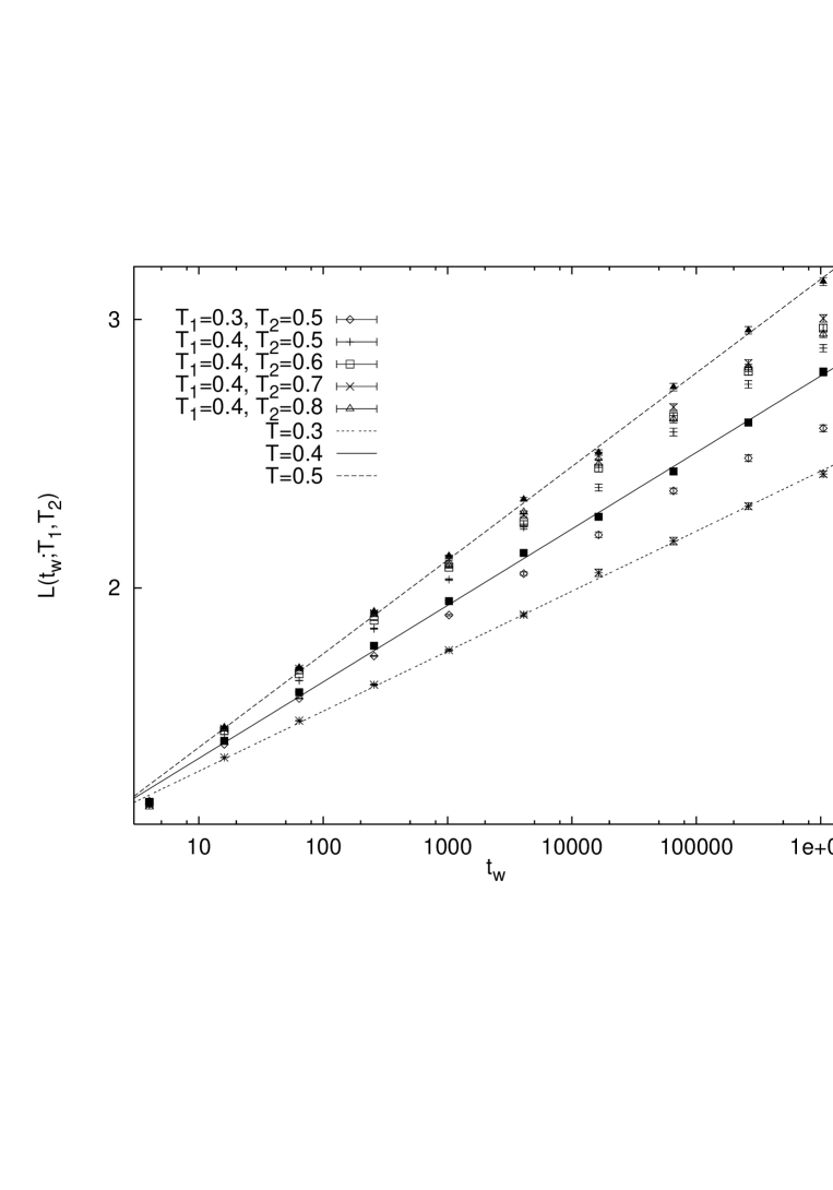
FIG. 9.: The overlap length $L(t_{w};T_{1},T_{2})$ of the 3D EA-model and the correlation length $\xi(t_{w})$ for different temperatures.

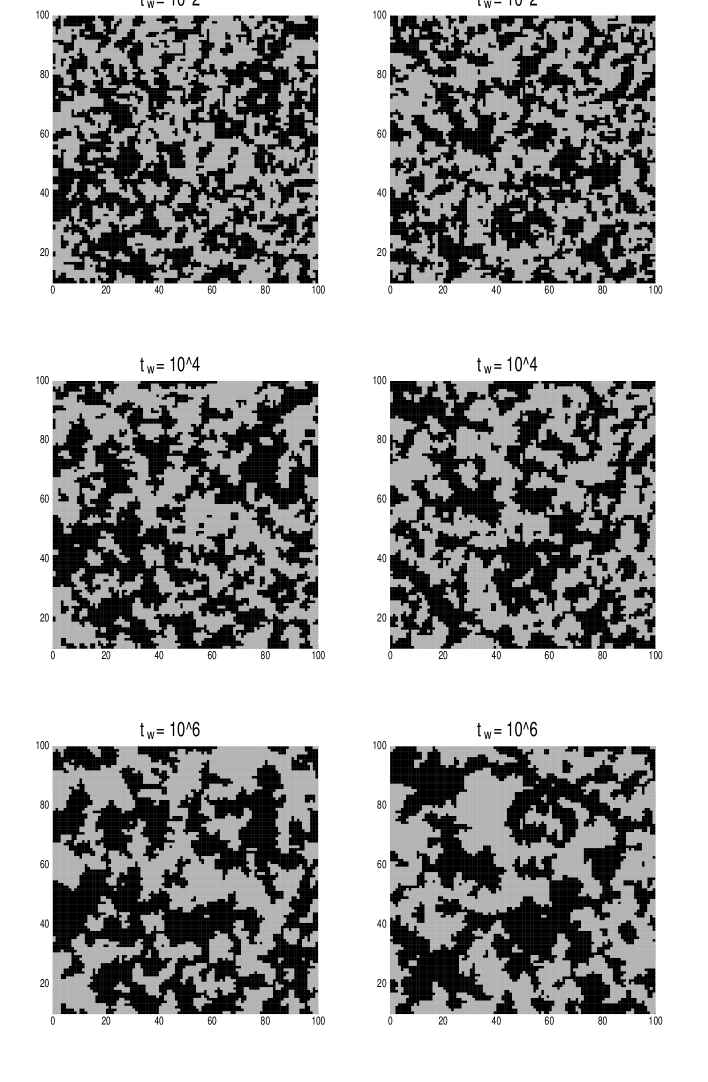
FIG. 10.: Domain growth in the 2D EA-model with Gaussian couplings. The right hand side shows the domains relative to the ground state and the left hand side shows the same configuration relative to a replica system.

FIG. 11.: The spatial correlation function $G(r,t_{w})$ of the 2D EA-model spin glass and temperatures $T=0.3$ and $T=0.8$. The waiting times are $t_{w}=5^{n}\quad\mbox{(n=1,\ldots,9)}$.

FIG. 12.: Algebraic (top) and logarithmic (bottom) fits of the correlation length $\xi(t_{w})$ of the 2D EA-model for different temperatures.

FIG. 13.: The correlation length $\xi(t_{w})$ of the 2D EA-model for higher temperatures.

FIG. 14.: Scaling plot of $G(r,t_{w})$ of the 2d EA-model for $T=0.3$

REFERENCES

- [1] K. Binder and A. P. Young, Rev. Mod. Phys. 58 (1986) 801.
- [2] For a recent review see H. Rieger, Monte Carlo studies of spin glasses and random field systems in Ann. Rev. Comp. Phys. II, 295 (1995), and references therein.
- [3] L. Lundgren, P. Svedlindh, P. Nordblad, and O. Beckmann, Phys. Rev. Lett. 51 (1983) 911.
- [4] L. C. E. Struik, Physical Aging in Amorphous Polymers and other materials, Elsevier, North-Holland (1978).
- [5] C. Rossel, Y. Maeno and I. Morgenstern, Phys. Rev. Lett. 62 (1989) 681.
- [6] K. Biljakovic, J. C. Lasjaunias, P. Monceau and F. Levy, Phys. Rev. Lett. 62 (1989) 1512 und 67 (1991) 1902.
- [7] P. Sibani and K. H. Hoffmann, Phys. Rev. Lett. 63 (1989) 2853
- [8] J. P. Bouchaud, J. Physique I 2 (1992) 1705 and J. P. Bouchaud and D. S. Dean, preprint cond-mat/9410022 (1994).
- [9] D. S. Fisher and D. A. Huse, Phys. Rev. B 38 (1988) 386 and Phys. Rev. B 38 (1988) 373.
- [10] G. J. M. Koper and H. J. Hilhorst, J. Phys. France 49 (1988) 429.
- [11] J. O. Andersson, J. Mattsson and P. Svedlindh, Phys. Rev. B 46 (1992) 8297.
- [12] H. Rieger, J. Phys. A 26 (1993) L615.
- [13] H. Rieger, B. Steckemetz and M. Schreckenberg, Europhys. Lett. 27 (1994) 485.
- [14] R. N. Bhatt and A. P. Young, Phys. Rev. B 37 (1988) 5606.
- [15] W. L. McMillan, Phys. Rev. B 31 (1985) 340 and Phys. Rev. B 30 (1984) 476.
- [16] A. J. Bray and M. A. Moore, Phys. Rev. B 31 (1985) 631.
- [17] L. Cugliandolo, J. Kurchan and F. Ritort, Phys. Rev. B 49 (1994) 6331.
- [18] H. Rieger, J. Kisker and M. Schreckenberg, Physica A 210 (1994) 326.
- [19] J. Kisker, H. Rieger and M. Schreckenberg, J. Phys. A 27 (1994) L853.
- [20] L. F. Cugliandolo, J. Kurchan and G. Parisi, J. Physique I (1994) 1641.
- [21] S. Franz and H. Rieger, J. Stat. Phys. 79 (1995) 749.
- [22] P. Granberg, P. Svedlindh, P. Nordblad, L. Lundgren and H. S. Chen, Phys. Rev. B 35 (1987) 2075.
- [23] K. Gunnarsson, P. Svedlindh, P. Nordblad and L. Lundgren, Phys. Rev. Lett. 61 (1988) 754.
- [24] A. Ito, H. Aruga, E. Torikai, M. Kikuchi, Y. Syono and H. Takei, Phys. Rev. Lett. 57 (1986) 483.
- [25] J. Mattson, T. Jonsson, P. Nordblad, H. A. Katori and A. Ito, Phys. Rev. Lett. 74 (1995) 4305.
- [26] P. Sibani and J. O. Andersson, Physica A 206 (1994) 1.
- [27] A. J. Bray and M. A. Moore, Phys. Rev. Lett. 58 (1987) 57.
- [28] H. Rieger, J. Physique I 4 (1994) 883.
- [29] F. Lefloch, J. Hammann, M. Ocio and E. Vincent, Europhys. Lett. 18 (1992) 647.
- [30] P. Refregier, E. Vincent, J. Hammann and M. Ocio, J. Physique 46 (1987) 1533.
- [31] E. Vincent, J. Hammann and M. Ocio in Recent Progress in Random Magnets (World Scientific, Singapore, 1992)
- [32] P. Granberg, L. Lundgren and P. Nordblad, J. Magnetism and Magnetic Materials 92 (1990) 228.
- [33] J. Mattson, C. Djurberg, P. Nordblad, L. Hoines, R. Stubi and J. A. Cowen, Phys. Rev. B 47 (1993) 14626.
- [34] J. O. Andersson, J. Mattson and P. Svedlindh, Physica B 194 (1994) 307.
- [35] C. De Simone, M. Diehl, M. Jünger, P. Mutzel, G. Reinelt and G. Rinaldi, J. Stat. Phys., in press (1995).
- [36] L. Cugliandolo and J. Kurchan, J. Phys. A 27 (1994) 5749. S. Franz and M. Mézard, Physica A 210 (1994) 43.