Representations of the quadratic Algebra and
Partially Asymmetric Diffusion with Open Boundaries
Fabian H.L. Eßler and Vladimir Rittenberg

Physikalisches Institut der Universität Bonn
Nussallee 12
53115 Bonn, GERMANY

ABSTRACT

We consider the one-dimensional partially asymmetric exclusion model with open boundaries. The model describes a system of hard-core particles that hop stochastically in both directions with different rates. At both boundaries particles are injected and extracted. By means of the method of Derrida, Evans, Hakim and Pasquier the stationary probability measure can be expressed as a matrix-product state involving two matrices forming a Fock-like representation of a general quadratic algebra. We obtain the representations of this algebra, which were unknown in the mathematical literature and use the two-dimensional one to derive exact expressions for the density profile and correlation functions. Using the correspondence between the stochastic model and a quantum spin chain, we obtain exact correlation functions for a spin-$\frac{1}{2}$ Heisenberg XXZ chain with non-diagonal boundary terms. Generalizations to other reaction-diffusion models are discussed.

PACS numbers: 05.40+j, 05.60.+w, 64.60, 75.10J

I Introduction

One dimensional reaction-diffusion processes recently have attracted much attention for a variety of reasons. Pure diffusion models have been studied in relation with interface growth [1], traffic-flow [2], the dynamics of shocks [3, 4], and magnetophoresis of tagged polymers [5]. More general reaction-diffusion models are of interest from a mathematical point of view due to their relation to integrable quantum chain hamiltonians [6]. It is interesting to note the important role played by the boundary conditions in these models [7], which completely control the physics in some cases. For the case of two-state models for example, in the corresponding quantum chain hamiltonians (which are XXZ models) the boundary conditions generally break the particle number $U(1)$ symmetry and are not easily treatable by the usual methods like the Bethe Ansatz [8, 9]. The problem is that although the chains can be shown to be integrable [10], the Bethe Ansatz so far has not been constructed due to the lack of a reference state.

An important step forward in these types of problems was made by Derrida, Domany and Mukamel [11] in the case of completely asymmetric diffusion with particle injection at one end of the chain, and particle extraction at the other end of the chain. They showed that there exists a recursion, which relates the probability distribution of the steady state for a $L$ sites to the one for $L-1$ sites. An equivalent formulation of this property was given by Derrida, Evans, Hakim and Pasquier (DEHP)[12], who demonstrated that the probability distribution can be written in a factorized form with coefficients that are not c-numbers but (infinite-dimensional) matrices. For the two-state model there are two matrices which form a Fock representation of the quadratic algebra. Using representations of this algebra one can compute in principle all correlation functions. In particular the density profile was determined in [12, 13], and in a special case (when the injection rate is equal to the extraction rate) even the two-point correlation function [14] was obtained. If one considers the more general problem with particle injection and extraction at both ends, and partially asymmetric diffusion, the DEHP approach is still applicable, but the representations of the quadratic algebra were not known. In a remarkable paper [15], Sandow was able to compute some important matrix elements in the envelopping algebra, which allowed him to compute the currents and to obtain the phase diagram, which coincides with the mean-field predictions.

In the present paper we start by determining all Fock representations of the most general quadratic algebra, which depends on seven parameters (section II). They might be of interest in other physical contexts as well. It turns out that the representations can be either finite-dimensional or infinite-dimensional. For each finite-dimensional representation one obtains a constraint equation for the seven parameters. This constraint depends on the dimension of the representation. The matrix elements of the two matrices appearing in the quadratic algebra are given by recursion relations. We show that for some special cases these recursions can be easily solved.

Next we review the connection between the steady-state probability distribution and the ground state of certain (in general non-hermitian) quantum chains (section III). In section IV we give a summary of the DEHP Ansatz and establish the connection with the quadratic algebra discussed in section II. In section V we consider the most general master equation for one-dimensional systems with two-body interactions (one has twelve independent rates) and particle injection and extraction at both boundaries and apply the DEHP Ansatz. One gets a quadratic algebra and two additional quadratic relations on the matrices. This implies that only finite-dimensional representations have a chance to be useful. We found that there exists a one-dimensional representation with three conditions for the twelve rates and the four parameters describing the injection and extraction of particles at the ends of the chain. The question of the existence of higher-dimensional representations and their physical relevance is left open. In Appendix B we study the applicability of the DEHP formalism to the steady state of a master equation with three-body interactions. We show that is this case one obtains, as expected, cubic algebras. Their representations and physical interest remains to be studied.

After these mathematical investigations we turn to a detailed study of the problem of partially asymmetric diffusion with particle injection/extraction at both boundaries. We start with a review of the known results in section VI, using the phase diagram obtained by Sandow [15] as a basis. In the following sections we concentrate on the application of the two-dimensional representation of the quadratic algebra to concrete calculations. In sections VII and VIII we show that as a result of the constraint equation for the existence of the representation one can cover parts of the phases $A_{II}$, $B_{II}$, the complete phases $A_{I}$ and $B_{I}$ as well as the coexistence line (in terms of the definitions of Schütz and Domany[13]). The calculation of the density profiles and two-point correlation functions in the low- and high-density phases is presented in section IX. One remarkable result is that the density around the center of the chain has a simple expression in terms of the parameters of the problem and that it coincides with the mean-field results (which are derived in Appendix F). The density profile and two-point function on the coexistence line are presented in section X.

Some by-products of our investigations are presented in the appendices. In Appendix C we give some identities concerning normal-ordered expressions of q-oscillators. In Appendix D we show how the DEHP Ansatz can be used to construct irreducible representations of the quantum group $U_{q}(SU(2))$. We close with a discussion of our results and some remarks on the time-dependence of correlation functions.

II Fock Representations of the quadratic Algebra

We are interested in Fock representations of the most general quadratic algebra

$$x_{1}A^{2}+x_{2}AB+x_{3}BA+x_{4}B^{2}=x_{5}A+x_{6}B+x_{7}\ ,$$ (1)

$$A|V\rangle\ =0\ ,\quad\langle W|B=0\ ,\quad\langle W|V\rangle\neq 0\ .$$ (2)

Here $x_{i}$ are complex parameters and quantities of physical interest are given by vacuum average values of monomials written in terms of $A$ and $B$, e.g.

$$\langle W|A^{r_{1}}B^{r_{2}}\ldots B^{r_{n}}|V\rangle\ .$$ (3)

Obviously (2) generalizes the algebra of creation and annihilation operators and its q-deformations. As far as we know the problem formulated above has not been considered in the mathematical literature (presumably because up to now there was no motivation to do so). General quadratic algebras were studied in [16] but no Fock-representations were considered. We will show in the present work that solving the above problem allows for the computation of concentration profiles and various correlation functions in the physical problem of partially asymmetric diffusion with open boundaries.

One can ask the question about the conditions on the $x_{i}$’s in (2) such that algebra determines the vacuum expectation value (3). This implies that the system of equations for words of length two, three, etc have solutions. Direct calculations show that an infinite set of inequalities have to be satisfied

$$x_{2}\neq 0\ ,\quad x_{1}x_{4}-x_{2}^{2}\neq 0\ ,\quad x_{2}(x_{2}^{2}-x_{1}x_{4})+(x_{3}-x_{2})x_{1}x_{4}\neq 0\ ,\quad{\sl etc}\ .$$ (4)

In section IV we will give, in a different parametrization, a simpler expression for these conditions. Instead of solving linear equations for words of different lengths it is useful to look for matrix representations of the algebra. Once those are known the calculation of the quantities (3) is simple. We are interested for obvious reasons in the representations of the smallest dimension because this is sufficient to compute the relevant quantities. As we are going to show the representations of the quadratic algebra are infinite-dimensional unless there exist certain constraints on the parameters $x_{i}$. The simplest such constraint is $x_{7}=0$, for which the representation is one-dimensional: $A=B=0$. From now on we will take $x_{7}\neq 0$. First we consider the case $x_{5}\neq 0\neq x_{6}$. We then define

$$\tilde{A}=\frac{x_{5}}{x_{7}}A\ ,\quad\tilde{B}=\frac{x_{6}}{x_{7}}B\ ,$$ (5)

in terms of which the algebra reads

$$z_{1}\tilde{A}^{2}+z_{2}\tilde{A}\tilde{B}+z_{3}\tilde{B}\tilde{A}+z_{4}\tilde{B}^{2}=\tilde{A}+\tilde{B}+1\ ,$$ (6)

where the $z_{i}$ are given in terms of the $x_{j}$ and where

$$\langle W|\tilde{B}=\tilde{A}|V\rangle\ =0,\quad\langle W|V\rangle\neq 0\ .$$ (7)

It is convenient to define

$$\xi=-\frac{z_{1}}{z_{2}}=-\frac{x_{1}x_{6}}{x_{2}x_{5}}\ ,\ \lambda=-\frac{z_{3}}{z_{2}}=-\frac{x_{3}}{x_{2}}\ ,\ \eta=-\frac{z_{4}}{z_{2}}=-\frac{x_{4}x_{5}}{x_{2}x_{6}}\ ,\ z_{2}=\frac{x_{2}x_{7}}{x_{5}x_{6}}\ .$$ (8)

One can show (see Appendix A) that through a similarity transformation the matrices $\tilde{A}$ and $\tilde{B}$ can be brought to a tridiagonal form with $|V\rangle=\pmatrix{1\cr 0\cr\vdots\cr 0}$ and $\langle W|=\pmatrix{1&0&\vdots&0}$. Using this fact together with equation (6) we obtain

$$\tilde{A}=\left(\matrix{a_{1}&f_{1}&0&0&0&0&0\ldots\cr\alpha_{1}\eta f_{1}&a_{2}&f_{2}&0&0&0&0\ldots\cr 0&\alpha_{2}\eta f_{2}&a_{3}&f_{3}&0&0&0\ldots\cr 0&0&\alpha_{3}\eta f_{3}&a_{4}&f_{4}&0&0\ldots\cr 0&0&0&\alpha_{4}\eta f_{4}&a_{5}&f_{5}&0\ldots\cr\ldots&&&&\ldots&&\cr}\right)$$ (9)

$$\tilde{B}=\left(\matrix{b_{1}&\alpha_{1}\xi f_{1}&0&0&0&0&0\ldots\cr f_{1}&b_{2}&\alpha_{2}\xi f_{2}&0&0&0&0\ldots\cr 0&f_{2}&b_{3}&\alpha_{3}\xi f_{3}&0&0&0\ldots\cr 0&0&f_{3}&b_{4}&\alpha_{4}\xi f_{4}&0&0\ldots\cr 0&0&0&f_{4}&b_{5}&\alpha_{5}\xi f_{5}&0\ldots\cr\ldots&&&&\ldots&&\cr}\right)\ .$$ (10)

The quantities $\alpha_{n},a_{n},b_{n}$ and $f_{n}$ are given recursively. First the $\alpha_{n}$’s are to be determined from

$$\alpha_{n}=\frac{1+\lambda\alpha_{n-1}}{1-\eta\xi\alpha_{n-1}}\ ,\ \alpha_{1}=0\ .$$ (11)

Next one determines $a_{n}$ and $b_{n}$ from

$$\pmatrix{a_{n+1}\cr b_{n+1}} = M\left[\left(\matrix{\xi(1-\alpha_{n})&\lambda+\eta\xi\alpha_{n}\cr\lambda+\eta\xi\alpha_{n}&\eta(1-\alpha_{n})\cr}\right)\pmatrix{a_{n}\cr b_{n}}+\frac{1}{z_{2}}\pmatrix{1+\xi\alpha_{n}\cr 1+\eta\alpha_{n}\cr}\right]\ ,$$ (12)

$$M = \frac{1}{\eta\xi(1+\lambda\alpha_{n})^{2}-(1-\eta\xi\alpha_{n})^{2}}\left(\matrix{-\eta(1+\lambda\alpha_{n})&-1+\eta\xi\alpha_{n}\cr-1+\eta\xi\alpha_{n}&-\xi(1+\lambda\alpha_{n})\cr}\right)\ ,$$ (13)

$$a_{1} = 0=b_{1}\ .$$ (14)

Finally the $f_{n}$’s are then given as

$$f_{n}^{2} = f_{n-1}^{2}\frac{\lambda+2\eta\xi\alpha_{n-1}-\eta\xi\alpha_{n-1}^{2}}{1-2\eta\xi\alpha_{n}-\lambda\eta\xi\alpha_{n}^{2}}+\frac{\xi a_{n}^{2}+\eta b_{n}^{2}+(\lambda-1)a_{n}b_{n}+\frac{a_{n}+b_{n}+1}{z_{2}}}{1-2\eta\xi\alpha_{n}-\lambda\eta\xi\alpha_{n}^{2}}\ ,$$ (15)

$$f_{0} = 0\ .$$ (16)

For later use we give the first few values

$$\alpha_{2} = 1\ ,\ \alpha_{3}=\frac{1+\lambda}{1-\eta\xi}\ ,$$ (17)

$$a_{2} = \frac{1+\eta}{z_{2}(1-\eta\xi)}\ ,\ b_{2}=\frac{1+\xi}{z_{2}(1-\eta\xi)}\ ,$$ (18)

$$f_{1}^{2} = \frac{1}{z_{2}}\ ,\ f_{2}^{2}=\frac{\lambda+1}{z_{2}^{2}(1-2\eta\xi-\lambda\eta\xi)}\left[z_{2}+\frac{(1+\xi)(1+\eta)}{(1-\eta\xi)^{2}}\right].$$ (19)

We note that for $\lambda=-1$ it follows that $f_{2}=0$ and we thus obtain only two-dimensional representations like for one fermion (observe the appearance of an anticommutator in (6)). The recursion (11) for $\alpha_{n}$ can be solved by redefining

$$\alpha_{n}=\frac{1}{\eta\xi}\left(1+\sqrt{\lambda+\eta\xi}\frac{u_{n+1}}{u_{n}}\right),$$ (20)

where the $u_{n}$’s satisfy the following recursion relation

$$u_{n+1}+u_{n-1} = -\frac{1+\lambda}{\sqrt{\lambda+\eta\xi}}u_{n}\ ,$$ (21)

$$u_{1} = 1\ ,\quad u_{2}=-\frac{1}{\sqrt{\lambda+\eta\xi}}\ .$$ (22)

This is recognized as the special case $x=-\frac{1+\lambda}{2(\lambda+\eta\xi)}$ of the recursion relation for Chebyshev polynomials $U_{n+1}(x)+U_{n-1}(x)=2xU_{n}(x)$. Using the representation $U_{n}(x)=\frac{\sin((n-1)\arccos(x)+\phi)}{\sin(\phi)}$ and taking into account the initial conditions we arrive at the result

$$\alpha_{n} = \frac{1}{\eta\xi}\left[1+\sqrt{\lambda+\eta\xi}\ \frac{\sin\left((n-1)\theta+\phi\right)}{\sin\left((n-2)\theta+\phi\right)}\right]\ ,$$ (23)

$$\phi = \arctan\left[\frac{\sqrt{4\eta\xi-(1-\lambda)^{2}}}{\lambda-1}\right]\ ,\ \theta=\arccos\left[-\frac{1+\lambda}{2\sqrt{\lambda+\eta\xi}}\right]\ .$$ (24)

The recursion (14) for $a_{n}$ and $b_{n}$ can be decoupled into recursion relations for ${\tilde{a}}_{n}=\sqrt{\xi}a_{n}+\sqrt{\eta}b_{n}$ and ${\tilde{b}}_{n}=\sqrt{\xi}a_{n}-\sqrt{\eta}b_{n}$:

$${\tilde{a}}_{n+1}=g^{+}_{n+1}{\tilde{a}}_{n}+h^{+}_{n+1}\ ,\ {\tilde{b}}_{n+1}=g^{-}_{n+1}{\tilde{b}}_{n}+h^{-}_{n+1}\ ,\$$ (25)

where $h^{\pm}_{n+1}=c_{1}\pm c_{2}$, $g^{\pm}_{n+1}=c_{3}\pm c_{4}$, and

$$c_{1} = -\sqrt{\xi}\frac{\eta(1+\lambda\alpha_{n})(1+\xi\alpha_{n})+(1-\eta\xi\alpha_{n})(1+\eta\alpha_{n})}{z_{2}(\eta\xi(1+\lambda\alpha_{n})^{2}-(1-\eta\xi\alpha_{n})^{2})}\,$$ (26)

$$c_{2} = -\sqrt{\eta}\frac{(1+\xi\alpha_{n})(1-\eta\xi\alpha_{n})+\xi(1+\eta\alpha_{n})(1+\lambda\alpha_{n})}{z_{2}(\eta\xi(1+\lambda\alpha_{n})^{2}-(1-\eta\xi\alpha_{n})^{2})}\,$$ (27)

$$c_{3} = -\frac{(\lambda+\eta\xi)(1-\eta\xi\alpha_{n}^{2})}{\eta\xi(1+\lambda\alpha_{n})^{2}-(1-\eta\xi\alpha_{n})^{2}}\ ,$$ (28)

$$c_{4} = -\frac{\sqrt{\eta\xi}(\lambda+1)(1+(\lambda-1)\alpha_{n}+\eta\xi\alpha_{n}^{2})}{\eta\xi(1+\lambda\alpha_{n})^{2}-(1-\eta\xi\alpha_{n})^{2}}\ .$$ (29)

It is hard to simplify the recursion relations further. Using the expression (24) for the $\alpha_{n}$’s and (29) one can derive formulae for $a_{n}$, $b_{n}$ and hence $f_{n}$. The resulting expressions are obviously very cumbersome. From the expressions (9) and (10) for $\tilde{A}$ and $\tilde{B}$ it follows that the condition for having an $n$-dimensional representation is simply $f_{n}=0$. As one can see from the form of the recurrence relations this constraint is a complicated function of $\lambda,\xi,\eta$ and $z_{2}$. This is the reason why we will use for applications only the two-dimensional representation ($f_{2}=0$), for which the matrix elements of $\tilde{A}$ and $\tilde{B}$ are given by (19).

Let us now consider the case $x_{5}=x_{6}=0$. The cases where only $x_{5}$ or $x_{6}$ vanishes can be studied in a similar way and thus will not be considered in detail here. The algebra for case $x_{5}=x_{6}=0$ is

$$z_{1}A^{2}+z_{2}AB+z_{3}BA+z_{4}B^{2}=1\ ,$$ (30)

where $z_{i}=\frac{x_{i}}{x_{7}}$. We define, like in (8)

$$\xi=-\frac{z_{1}}{z_{2}}\ ,\ \lambda=-\frac{z_{3}}{z_{2}}\ ,\ \eta=-\frac{z_{4}}{z_{2}}\ .$$ (31)

The infinite-dimensional representation of (30) is of the form (9)-(10) with vanishing diagonal terms $a_{n}=b_{n}=0\ ,\forall n$, where $\eta,\xi,\lambda$ are defined in (31) and where $\alpha_{n}$ and $f_{n}$ are given by

$$\alpha_{n} = \frac{1+\lambda\alpha_{n-1}}{1-\eta\xi\alpha_{n-1}}\ ,\ \alpha_{1}=0\ ,$$ (32)

$$f_{n}^{2} = f_{n-1}^{2}\frac{\lambda+2\eta\xi\alpha_{n-1}-\eta\xi\alpha_{n-1}^{2}}{1-2\eta\xi\alpha_{n}-\lambda\eta\xi\alpha_{n}^{2}}+\frac{1}{z_{2}(1-2\eta\xi\alpha_{n}-\lambda\eta\xi\alpha_{n}^{2})}\ ,\ f_{0}^{2}=0\ .$$ (33)

Apart from this infinite-dimensional representation there are two kinds of finite-dimensional ones. The first kind is simply obtained by imposing the constraint $f_{N}=0$ on the parameters $z_{i}$, which leads to the decoupling of an $N\times N$ block in the upper left corner of the infinite-dimensional representation of $A$ and $B$ discussed above. The resulting finite-dimensional representation is given in terms of $N\times N$ matrices $A$ and $B$ with vanishing diagonal elements.

The matrices $A$ and $B$ of the second type of $N\times N$ representation take the following form

$$A=\left(\matrix{0&f_{1}&0&0&0&0&0\ldots&&\cr\alpha_{1}\eta f_{1}&0&f_{2}&0&0&0&0\ldots&&\cr 0&\alpha_{2}\eta f_{2}&0&f_{3}&0&0&0\ldots&&\cr 0&0&\alpha_{3}\eta f_{3}&0&f_{4}&0&0\ldots&&\cr 0&0&0&\alpha_{4}\eta f_{4}&0&f_{5}&0\ldots&&\cr\ldots&&&&\ldots&&&&\cr\ldots&&&&\ldots&&&&\cr\ldots&&&&\ldots&&\alpha_{N-2}\eta f_{N-2}&0&f_{N-1}\cr\ldots&&&&\ldots&&0&\alpha_{N-1}\eta f_{N-1}&a_{N}\cr}\right)\ ,$$ (34)

$$B=\left(\matrix{0&\alpha_{1}\xi f_{1}&0&0&0&0&0\ldots&&\cr f_{1}&0&\alpha_{2}\xi f_{2}&0&0&0&0\ldots&&\cr 0&f_{2}&0&\alpha_{3}\xi f_{3}&0&0&0\ldots&&\cr 0&0&f_{3}&0&\alpha_{4}\xi f_{4}&0&0\ldots&&\cr 0&0&0&f_{4}&0&\alpha_{5}\xi f_{5}&0\ldots&&\cr\ldots&&&&\ldots&&&&\cr\ldots&&&&\ldots&&&&\cr\ldots&&&&\ldots&&f_{N-2}&0&\alpha_{N-1}\xi f_{N-1}\cr\ldots&&&&\ldots&&0&f_{N-1}&b_{N}&\cr}\right)\ ,$$ (35)

where $\alpha_{n}$ and $f_{n}$ are determined by the recursion (33). The representation (34), (35) exists provided that

$$\alpha_{N}^{2}\eta\xi=1\ .$$ (36)

The variables $a_{N}$ and $b_{N}$ are obtained from the equations

$$b_{N} = \xi\alpha_{N}a_{N}\ ,$$ (37)

$$\left(-\lambda-2\xi\eta\alpha_{N-1}+\eta\xi\alpha_{N-1}^{2}\right)f_{N-1}^{2} = \xi a_{N}^{2}+\eta b_{N}^{2}+(\lambda-1)a_{N}b_{N}+\frac{1}{z_{2}}\ .$$ (38)

We are going to close this section with two cases, for which the recurrence relations can be solved in a trivial way.

• If $\lambda=-\eta\xi\neq-1$ (this case is as we will see physically interesting) the following simplifications take place for $x_{5}\neq 0\neq x_{6}$:

  $$a_{n} = a=\frac{1+2\eta-\lambda}{z_{2}(1+\lambda)^{2}}\ ,\ \forall n\geq 3\ ,a_{1}=0,\ a_{2}=\frac{1+\eta}{z_{2}(1+\lambda)}\ ,$$ (39)

  $$b_{n} = b=\frac{1+2\xi-\lambda}{z_{2}(1+\lambda)^{2}}\ ,\ \forall n\geq 3\ ,b_{1}=0,\ b_{2}=\frac{1+\xi}{z_{2}(1+\lambda)}\ ,$$ (40)

  $$f_{n}^{2} = f^{2}=\frac{\xi a^{2}+\eta b^{2}+(\lambda-1)ab+\frac{a+b+1}{z_{2}}}{(1+\lambda)^{2}}\ ,\ \forall n\geq 3\ ,$$ (41)

  $$f_{1}^{2} = \frac{1}{z_{2}},\ f_{2}^{2}=\frac{1}{z_{2}(1+\lambda)^{2}}\left(1+\lambda+\frac{1+\xi+\eta-\lambda}{z_{2}(1+\lambda)}\right)\ .$$ (42)

  Note that in this case there exist only 2-d ($f_{2}=0$), 3-d ($f_{3}=0$), and infinite-dimensional representations ! If $x_{5}=x_{6}=0$, one has an infinite-dimensional representation with vanishing diagonal elements $a_{n}=b_{n}=0\ ,\ \forall n$ with

  $$\alpha_{n}=1\ \forall n\geq 2,\quad f_{1}^{2}=\frac{1}{z_{2}}\ ,\ f_{2}^{2}=\frac{1}{z_{2}(1+\lambda)}\ ,\ f_{n}^{2}=\frac{1}{z_{2}(1+\lambda)^{2}}\ ,\ \forall n\geq 3\ ,$$ (43)

  where $\eta,\xi,\lambda$ are given by (31).

• $0=\eta=\xi$

  Here it is possible to choose $\tilde{B}=\tilde{A}^{\dagger}$, and

  $$\alpha_{n} = \frac{1-\lambda^{n-1}}{1-\lambda}\ ,\ a_{n}=\frac{1}{z_{2}}\left(\frac{1-\lambda^{n-1}}{1-\lambda}\right)\ ,\quad f_{n}^{2}=\frac{1}{z_{2}}\left(\frac{1-\lambda^{n}}{1-\lambda}\right)\left(1+\frac{1}{z_{2}}\frac{1-\lambda^{n-1}}{1-\lambda}\right),$$ (44)

  where we have assumed $x_{5}\neq 0\neq x_{6}$. A similar simplification holds if $x_{5}=0$ or $x_{6}=0$. Of particular physical interest is the case $\lambda=1$, which exhibits additional simplifications

  $$\alpha_{n}=n-1\ ,\qquad a_{n}=\frac{n-1}{z_{2}}\ ,\ f_{n}^{2}=\frac{n}{z_{2}}+\frac{n(n-1)}{z_{2}^{2}}\ .$$ (45)

III The Master Equation and the Quantum Chain Hamiltonian

Let us consider a one-dimensional open chain with $L$ sites. On each site $k(k=1,2,...L)$ we allow for two configurations described by means of the variable $\tau_{k}$, which takes the two values $0$ and $1$. For $\tau_{k}=0$ the site $k$ is empty (vacancy), for $\tau_{k}=1$ the site $k$ is occupied by a molecule $A$.

At time $t$ the probability to find a certain configuration of molecules and vacancies on the chain is given by the probability distribution

$$P_{L}\left(\tau_{1},\tau_{2},\ldots\tau_{L}|t\right)\ .$$ (46)

If we assume that interaction between molecules is described by two-body processes only (three-body processes are considered in Appendix B), the time evolution of the system is given by a master equation of the form

$$\frac{\partial P_{L}}{\partial t} = -\sum_{k=1}^{L-1}\sum_{\gamma_{k},\gamma_{k+1}}\left(H_{k,k+1}\right)_{\tau_{k},\tau_{k+1}}^{\gamma_{k},\gamma_{k+1}}P_{L}(\tau_{1},\tau_{2}\ldots\tau_{k-1},\gamma_{k},\gamma_{k+1},\tau_{k+2}\ldots\tau_{L}|t)$$ (48)

$$-\sum_{\gamma_{1}}\left(h_{1}\right)_{\tau_{1}}^{\gamma_{1}}P_{L}(\gamma_{1},\tau_{2}\ldots\tau_{L}|t)-\sum_{\gamma_{L}}\left(h_{L}\right)_{\tau_{L}}^{\gamma_{L}}P_{L}(\tau_{1},\tau_{2}\ldots\tau_{L-1},\gamma_{L}|t)\ ,$$

where the boundary contributions $h_{1}$ and $h_{L}$ describe injection (extraction) of particles with rates $\alpha$ and $\delta$ ($\gamma$ and $\beta$) at sites $1$ and $L$

$$h_{1}=\left(\matrix{\alpha&-\gamma\cr-\alpha&\gamma\cr}\right)\ ,\ h_{L}=\left(\matrix{\delta&-\beta\cr-\delta&\beta\cr}\right)\ ,$$ (49)

and where

$$\left(H_{k,k+1}\right)_{\tau_{k},\tau_{k+1}}^{\gamma_{k},\gamma_{k+1}}=\Bigg{\{}{\matrix{\sum^{\prime}_{\beta_{k},\beta_{k+1}}[{\Gamma_{k,k+1}}]_{\beta_{k},\beta_{k+1}}^{\gamma_{k},\gamma_{k+1}}\qquad\gamma_{j}=\tau_{j}\ ,\ j=k,k+1\cr-[{\Gamma_{k,k+1}}]_{\tau_{k},\tau_{k+1}}^{\gamma_{k},\gamma_{k+1}}\qquad{\rm else}\cr}}$$ (50)

Here $[\Gamma_{k,k+1}]^{\gamma_{k},\gamma_{k+1}}_{\tau_{k},\tau_{k+1}}$ represents the probability per unit time that the configuration $(\gamma_{k},\gamma_{k+1})$ on neighbouring sites $k$ and $k+1$ changes into the configuration $(\tau_{k},\tau_{k+1})$ and $\sum^{\prime}$ denotes the sum where the term $(\gamma_{k},\gamma_{k+1})=(\beta_{k},\beta_{k+1})$ is excluded. The following processes are included in the master equation (with $0$ a vacancy $(\tau=0)$ and $A$ a molecule $(\tau=1)$)

$$\begin{array}[]{lcr}{\mbox{Diffusion to the right:}}&A+0\to 0+A&({\mbox{rate}}\;\Gamma^{10}_{01})\\ {\mbox{Diffusion to the left:}}&0+A\to A+0&(\Gamma^{01}_{10})\\ {\mbox{Coagulation at the right:}}&A+A\to 0+A&(\Gamma^{11}_{01})\\ {\mbox{Coagulation at the left:}}&A+A\to A+0&(\Gamma^{11}_{10})\\ {\mbox{Decoagulation at the right:}}&A+0\to A+A&(\Gamma^{10}_{11})\\ {\mbox{Decoagulation at the left:}}&0+A\to A+A&(\Gamma^{01}_{11})\\ {\mbox{Birth at the right:}}&0+0\to 0+A&(\Gamma^{00}_{01})\\ {\mbox{Birth at the left:}}&0+0\to A+0&(\Gamma^{00}_{10})\\ {\mbox{Death at the right:}}&0+A\to 0+0&(\Gamma^{01}_{00})\\ {\mbox{Death at the left:}}&A+0\to 0+0&(\Gamma^{10}_{00})\\ {\mbox{Pair-annihilation:}}&A+A\to 0+0&(\Gamma^{11}_{00})\\ {\mbox{Pair-creation:}}&0+0\to A+A&(\Gamma^{00}_{11})\end{array}$$ (51)

Reaction-diffusion models of the type described above can be mapped to quantum spin chains in the following way [6]: a basis of the quantum-mechanical Hilbert space ${\cal H}$ (isomorphic to the tensor product $\otimes_{n=1}^{L}C^{2}$) is defined as

$$|\{\tau\}\rangle=|\tau_{1}\ldots\tau_{L}\rangle\ ,$$ (52)

and the inner product is taken as

$$\langle\{\tau\}|\{\tau^{\prime}\}\rangle=\prod_{j=1}^{L}\delta_{\tau_{j},\tau_{j}^{\prime}}.$$ (53)

This induces a map of the probability distribution $P_{L}$ to a state in ${\cal H}$

$$|P\rangle=\sum_{\{\tau\}}P_{L}(\tau_{1}\ldots\tau_{L}|t)|\{\tau\}\rangle\ ,$$ (54)

and the master equation (48) then implies an imaginary-time Schrödinger equation

$$\frac{\partial|P\rangle}{\partial t}=-{\hat{H}}|P\rangle\ .$$ (55)

Here ${\hat{H}}$ is a quantum hamiltonian defined in terms of a basis $E_{k}^{\alpha\beta}$ (which can be represented as $2\times 2$ matrices with entries ${E^{\alpha\beta}}_{\gamma\delta}=\delta_{\alpha\gamma}\delta_{\beta\delta}$) of quantum operators on the $k$’th site of the lattice via

$${\hat{H}}=\sum_{k=1}^{L-1}(H_{k,k+1})^{\alpha\beta}_{\gamma\delta}E_{k}^{\gamma\alpha}E_{k+1}^{\delta\beta}+(h_{1})^{\alpha}_{\gamma}E_{1}^{\gamma\alpha}+(h_{L})^{\alpha}_{\gamma}E_{L}^{\gamma\alpha}\ ,$$ (56)

where $h_{1}$, $h_{L}$ and $H_{k,k+1}$ are defined in (50). Note that in general the hamiltonian ${\hat{H}}$ will be non-hermitian. It is easy to see that

$$\langle 0|{\hat{H}}=0\ ,$$ (57)

where $\langle 0\mid$ is given by

$$\langle 0\mid=\sum_{\{\tau\}}\langle\{\tau\}\mid\;=\;\left\langle{1\choose 1}\otimes\right.{1\choose 1}\otimes\ldots\otimes{1\choose 1}\mid$$ (58)

Using (55) it follows from (57) that $\langle 0|$ is a left “stationary” state. Assuming that this is the unique left “stationary” state and given a unique right stationary state

$$|0\rangle=\sum_{\{\tau\}}P_{s}(\{\tau\})|\{\tau\}\rangle$$ (59)

the average of the observable $X\left(\tau_{1},\ldots\tau_{L}\right)=X(\{\tau\})$ is defined as

$$\langle X\rangle = \sum_{\{\tau\}}X(\{\tau\})P_{s}(\{\tau\})$$ (60)

$$= \langle 0\mid X\mid 0\rangle\ .$$ (61)

An example, with which we will be concerned in most of this paper is the case of partially asymmetric diffusion, which corresponds to the choice of rates

$$[{\Gamma_{k,k+1}}]^{10}_{01}=p\ ,\ [{\Gamma_{k,k+1}}]^{01}_{10}=q$$ (62)

(all other rates are taken to be zero) the quantum hamiltonian ${\hat{H}}$ obtained by the above mapping is related to an XXZ spin chain by a similarity transformation

$$H_{XXZ}=U{\hat{H}}U^{-1}\ ,\ U=\prod_{j=1}^{L}\left(E_{j}^{00}+E_{j}^{11}\Lambda{\cal Q}^{j-1}\right)=\prod_{j=1}^{L}\left(\matrix{1&0\cr 0&\Lambda{\cal Q}^{j-1}\cr}\right)$$ (63)

where ${\cal Q}=\sqrt{\frac{q}{p}}$, $\Lambda$ is a free parameter and

$$\frac{1}{\sqrt{pq}}H_{XXZ} = -\frac{1}{2}\sum_{j=1}^{L-1}\biggl{[}2(\sigma^{+}_{j}\sigma^{-}_{j+1}+\sigma^{-}_{j}\sigma^{+}_{j+1})+\frac{1}{2}({\cal Q}+{\cal Q}^{-1})\sigma^{z}_{j}\sigma^{z}_{j+1}$$ (65)

$$\qquad\qquad+\frac{{\cal Q}-{\cal Q}^{-1}}{2}(\sigma_{j+1}^{z}-\sigma_{j}^{z})-\frac{1}{2}({\cal Q}+{\cal Q}^{-1})\biggr{]}+B_{1}+B_{L}$$

$$B_{1} = \sigma_{1}^{z}\frac{\alpha-\gamma}{2\sqrt{pq}}-\sigma_{1}^{-}\frac{\Lambda\alpha}{\sqrt{pq}}-\sigma_{1}^{+}\frac{\gamma}{\Lambda\sqrt{pq}}+\frac{\alpha+\gamma}{2\sqrt{pq}}\ ,$$ (66)

$$B_{L} = \sigma_{L}^{z}\frac{\delta-\beta}{2\sqrt{pq}}-\sigma_{L}^{-}\frac{\Lambda\delta}{\sqrt{pq}}{\cal Q}^{L-1}-\sigma_{L}^{+}\frac{\beta}{\Lambda\sqrt{pq}}{\cal Q}^{1-L}+\frac{\beta+\delta}{2\sqrt{pq}}\ .$$ (67)

This is the $U_{q}(SU(2))$ invariant quantum spin chain [17] with added boundary terms $B_{1}$ and $B_{L}$. Notice that the boundary terms contain nondiagonal contributions ($\sigma_{1}^{\pm}$, $\sigma_{L}^{\pm}$) with $L$-dependent coefficients. In the absence of the boundary terms the spectrum of the hamiltonian is massive. As is shown below the boundary terms with generate phase transitions with massless phases. Although the hamiltonian (67) can be shown to be integrable [10], the Bethe Ansatz so far has not been constructed due to the lack of a reference state.

We note that the similarity transformation (63) does not change averages of observables

$$\langle 0|X|0\rangle=\langle 0|U^{-1}UXU^{-1}U|0\rangle=\ _{U}\!\langle 0|X_{U}|0\rangle_{U}\ .$$ (68)

Thus zero-temperature equal time correlation functions of the XXZ quantum spin chain and (stationary-state) averages of the partially asymmetric diffusion model are related in the following way

$$\langle\sigma^{z}_{j}\rangle = {}_{U}\!\langle 0|\sigma^{z}_{j}|0\rangle_{U}=2\langle\tau_{j}\rangle-1\ ,$$ (69)

$$\langle\sigma^{z}_{j}\sigma^{z}_{k}\rangle = {}_{U}\!\langle 0|\sigma^{z}_{j}\sigma^{z}_{k}|0\rangle_{U}=4\langle\tau_{j}\tau_{k}\rangle+1-2\langle\tau_{j}\rangle-2\langle\tau_{k}\rangle\ ,$$ (70)

$$\langle\sigma^{z}_{j}\sigma^{z}_{k}\rangle_{conn} = 4\langle\tau_{j}\tau_{k}\rangle_{conn}\ ,$$ (71)

where _conn denotes connected correlation functions. This means that all results concerning averages in the partially asymmetric diffusion model obtained in this paper can be immediately applied to the case of the XXZ chain described above.

IV The DEHP Ansatz

In a remarkable paper [12] it was shown that for the case of asymmetric diffusion the problem of determining the probability distribution $P_{L}(\tau_{1},\ldots\tau_{L})$ for a stationary state can be formulated in a completely algebraic framework. We now briefly review the relevant results. All rates except $[\Gamma_{k,k+1}]^{10}_{01}=p$ and $[\Gamma_{k,k+1}]^{01}_{10}=q$ ($k=1,\ldots L-1$) are taken to be zero, and the boundary conditions are chosen according to (49): particles are injected at sites $1$ and $L$ with rates $\alpha$ and $\delta$ and extracted with rates $\gamma$ and $\beta$ respectively. The algebraization of the problem of determining the unnormalized probability distribution $P_{L}(\tau_{1}\ldots\tau_{L})$ of a stationary state is performed in two steps: one first makes an Ansatz $P_{L}(\tau_{1},\ldots\tau_{L})$ in the form of a matrix-product state [12, 18]

$$P_{L}(\tau_{1},...,\tau_{L}) = \langle W|\prod_{i=1}^{L}(\tau_{i}D+(1-\tau_{i})E)|V\rangle\ .$$ (72)

Here $D$ and $E$ are in general infinite-dimensional matrices and $\langle W|$ and $|V\rangle$ are vectors connected with the boundary conditions. The normalization factor is obviously given by

$$Z_{L}=\langle W|C^{L}|V\rangle\ ,\qquad C=D+E\ .$$ (73)

In the second step the following sufficient conditions for $P_{L}$ to be a stationary solution of the master equation are imposed

$$\sum_{\gamma_{k},\gamma_{k+1}}\left(H_{k,k+1}\right)_{\tau_{k},\tau_{k+1}}^{\gamma_{k},\gamma_{k+1}} P_{L}(\tau_{1},\tau_{2}\ldots\tau_{k-1},\gamma_{k},\gamma_{k+1},\tau_{k+2}\ldots\tau_{L})$$ (74)

$$= x_{\tau_{k}}P_{L-1}(\tau_{1}\ldots\tau_{k-1}\tau_{k+1}\ldots\tau_{L})-x_{\tau_{k+1}}P_{L-1}(\tau_{1}\ldots\tau_{k}\tau_{k+2}\ldots\tau_{L})\ ,$$ (77)

$$\sum_{\gamma_{1}}(h_{1})_{\tau_{1}}^{\gamma_{1}}P_{L}(\gamma_{1}\tau_{2}\ldots\tau_{L})=-x_{\tau_{1}}P_{L-1}(\tau_{2}\ldots\tau_{L})$$

$$\sum_{\gamma_{L}}(h_{L})_{\tau_{L}}^{\gamma_{L}}P_{L}(\tau_{1}\ldots\tau_{L-1}\gamma_{L})=x_{\tau_{L}}P_{L-1}(\tau_{1}\ldots\tau_{L-1})\ .$$

Inserting (72) into (77) , (77) leads to algebraic relations between the matrices $D$ and $E$ and leads to conditions for the action of $D$ and $E$ on $|V\rangle$ and $\langle W|$ [12] (one finds that $x_{0}=-x_{1}$ and then sets $x_{1}=1$)

$$pDE-qED = D+E$$ (78)

$$(\beta D-\delta E)|V\rangle = |V\rangle$$ (79)

$$\langle W|(\alpha E-\gamma D) = \langle W|$$ (80)

$$\langle W|V\rangle \neq 0\ .$$ (81)

It is easy to see that for $\alpha\beta=\gamma\delta$ no representations of (81) exist. This can be seen by considering the inner product

$$\langle W|\left(\alpha E-\gamma D\right)|V\rangle\ .$$ (82)

Evaluating (82) once by acting to the left and once by acting to the right using that $\alpha E-\gamma D=-\frac{\gamma}{\beta}(\beta D-\delta E)$ (which holds because $\alpha\beta=\gamma\delta$) we obtain

$$\langle W|V\rangle=-\frac{\gamma}{\beta}\langle W|V\rangle\ ,$$ (83)

which has the only solution $\langle W|V\rangle=0$. This means that from now on we can constrain ourselves without loss of generality to the case $\alpha\beta\neq\gamma\delta$. Moreover one can show that all vacuum expectation values

$$\langle W|D^{r_{1}}E^{r_{2}}\ldots D^{r_{n}}|V\rangle$$ (84)

are determined by (81) if the following inequalities are satisfied

$$p^{k}\alpha\beta-q^{k}\gamma\delta\neq 0\ ,\quad k=0,1,2,\ldots$$ (85)

The proof uses the construction of [15] and one can show that if (85) is satisfied a representation exists even if its dimension is not the one of the smallest representation. In order to obtain $P_{L}$ it is now necessary to find matrices $D$ and $E$ together with vectors $\langle W|$ and $|V\rangle$ obeying (81).

For later use we note that physical quantities like the current $J$, density profile $\langle\tau_{j}\rangle$ and two-point function $\langle\tau_{j}\tau_{k}\rangle$ can be evaluated in the following way [12]

$$J = \frac{\langle W|C^{L-1}|V\rangle}{\langle W|C^{L}|V\rangle}\ ,$$ (86)

$$\langle\tau_{j}\rangle = \frac{\langle W|C^{j-1}DC^{L-j}|V\rangle}{\langle W|C^{L}|V\rangle}\ ,$$ (87)

$$\langle\tau_{j}\tau_{k}\rangle = \frac{\langle W|C^{j-1}DC^{k-j-1}DC^{L-k}|V\rangle}{\langle W|C^{L}|V\rangle}\ ,$$ (88)

where $C=D+E$.

It is possible to determine certain matrix elements of representations of the six-parametric algebra (81) directly. This was done by Sandow [15] who then was able to determine both the current $J$ (the computations of which involves only the matrix $C$) in the infinite volume limit $L\rightarrow\infty$ and, remarkably, the phase diagram of the system. In order to compute the density profile and the two-point function a much more detailed understanding of the representations is needed. In order to study representation theory of (81) we introduce two operators $A$ and $B$, which act trivially on $\langle W|$ and $|V\rangle$ respectively

$$A = \beta D-\delta E-1\ ,\ B=\alpha E-\gamma D-1\ ,$$ (89)

$$\langle W|B = 0=A|V\rangle\ ,$$ (90)

If $A$ and $B$ are known, one can get $D$ and $E$ since $\alpha\beta\neq\gamma\delta$. $A$ and $B$ are seen to obey the quadratic algebra (2) discussed in section II with

$$x_{1} = (p-q)\alpha\gamma\ ,\quad x_{2}=p\alpha\beta-q\gamma\delta\ ,\quad x_{3}=p\gamma\delta-q\alpha\beta\ ,\quad x_{4}=(p-q)\beta\delta\ ,$$ (91)

$$x_{5} = (\alpha+\gamma)(\alpha\beta-\gamma\delta)-(p-q)[\gamma(\alpha+\delta)+\alpha(\beta+\gamma)]\ ,$$ (92)

$$x_{6} = (\beta+\delta)(\alpha\beta-\gamma\delta)-(p-q)[\beta(\alpha+\delta)+\delta(\beta+\gamma)]\ ,$$ (93)

$$x_{7} = (\alpha+\beta+\gamma+\delta)(\alpha\beta-\gamma\delta)-(p-q)(\alpha+\delta)(\beta+\gamma)\ .$$ (94)

Note that the seven parameters $x_{i}$ are not independent, since they depend only on six variables $p,q,\alpha,\beta,\gamma,\delta$. Conversely the algebra (2) can be brought to the form (81) if

$$(x_{2}+x_{3})^{2}-4x_{1}x_{4}\neq 0\ .$$ (95)

One can easily verify that the inequalities (95) and (4) correspond to those of (85) for $k=0,1,2,3$.

We now observe that in the case $q=0$ of completely asymmetric diffusion we have $\lambda=-\eta\xi$ and the matrices $\tilde{A}$ and $\tilde{B}$ (which we recall were defined as $\tilde{A}=\frac{x_{5}}{x_{7}}A$ and $\tilde{B}=\frac{x_{6}}{x_{7}}B$) have the simple forms given by (42). The origin of this simplification can be traced back to the representation theory of quantum groups which also simplifies drastically in the crystal basis $q=0$ [20]. Another case for which $A$ and $B$ have a simple form is $p=q$ (symmetric diffusion). Here we have $\xi=\eta=0$,$\lambda=1$, and the representation is given by (45). Finally, if $\alpha=\beta=p-q$, $\gamma=\delta=0$, we can define

$$a=\sqrt{\frac{p}{p-q}}A\ ,\ a^{\dagger}=\sqrt{\frac{p}{p-q}}B$$ (96)

and the algebra (2) is rewritten as a Q-oscillator algebra[21, 22, 23]

$$aa^{\dagger}-Qa^{\dagger}a=1\ ,$$ (97)

where $Q=\frac{q}{p}$. The vectors $|V\rangle$ and $\langle W|$ turn into usual Fock-vacua $\langle 0|$ and $|0\rangle$ defined by $a|0\rangle=\langle 0|a^{\dagger}=0$. Some observations about this case can be found in Appendix C.

As noticed before in section III, in the absence of boundary terms the hamiltonian (67) is $U_{q}(SU(2))$ invariant. The ground state of this hamiltonian is $L+1$ times degenerate (recall that $L$ is the length of the lattice) corresponding to a $L+1$-dimensional representation of the algebra. We demonstrate in Appendix D that this representation can also be found through the DEHP-Ansatz.

V Further Applications of the DEHP Ansatz

It is an interesting question, to what extent the Ansatz (72) can be used to describe more general reaction-diffusion models of the type (51). Inserting (72) into the master equation (77) for a general reaction-diffusion process defined via (49)-(51) (note that we take all rates constant throughout the bulk, i.e., $[\Gamma_{k,k+1}]^{\alpha\beta}_{\gamma\delta}=\Gamma^{\alpha\beta}_{\gamma\delta}$), we obtain the algebra

$${\cal H}\pmatrix{E^{2}\cr ED\cr DE\cr D^{2}\cr}=\pmatrix{0\cr x_{0}D-x_{1}E\cr-x_{0}D+x_{1}E\cr 0\cr}\ ,$$ (98)

$${\cal H}\!=\!\left(\matrix{\Gamma^{00}_{01}\!+\!\Gamma^{00}_{10}\!+\!\Gamma^{00}_{11}&\!\!-\Gamma^{01}_{00}&\!\!-\Gamma^{10}_{00}&\!\!-\Gamma^{11}_{00}\cr-\Gamma^{00}_{01}&\!\!\Gamma^{01}_{00}\!+\!\Gamma^{01}_{10}\!+\!\Gamma^{01}_{11}&\!\!-\Gamma^{10}_{01}&\!\!-\Gamma^{11}_{01}\cr-\Gamma^{00}_{10}&\!\!-\Gamma^{01}_{10}&\!\!\Gamma^{10}_{00}\!+\!\Gamma^{10}_{01}\!+\!\Gamma^{10}_{11}&\!\!-\Gamma^{11}_{10}\cr-\Gamma^{00}_{11}&\!\!-\Gamma^{01}_{11}&\!\!-\Gamma^{10}_{11}&\!\!\Gamma^{11}_{00}\!+\!\Gamma^{11}_{01}\!+\!\Gamma^{11}_{10}\cr}\right),$$ (99)

whereas the boundary conditions (77) impose the following conditions on the vectors $|V\rangle$ and $\langle W|$

$$\sum_{\gamma_{1}}(h_{1})_{\tau_{1}}^{\gamma_{1}}\langle W|[\gamma_{1}D+(1-\gamma_{1})E]=-x_{\tau_{1}}\langle W|$$ (100)

$$\sum_{\gamma_{L}}(h_{L})_{\tau_{L}}^{\gamma_{L}}[\gamma_{L}D+(1-\gamma_{L})E]|V\rangle=x_{\tau_{L}}|V\rangle\ .$$ (101)

Here $h_{1}$ and $h_{L}$ are given by (49) and thus (101) are independent from (99). From (101) it follows that $x_{0}=-x_{1}$, so that we can choose $x_{0}=-1$, $x_{1}=1$ by fixing the overall normalization in (77).

It is easily seen that only three equations of (99) are linearly independent. These can be cast in the form

$$\kappa_{1}DE+\kappa_{2}ED = D+E\ ,$$ (102)

$$\kappa_{3}D^{2} = \kappa_{4}DE+\kappa_{5}ED\ ,$$ (103)

$$\kappa_{6}E^{2} = \kappa_{7}DE+\kappa_{8}ED\ ,$$ (104)

where $\kappa_{j}$ are given in terms of the rates $\Gamma^{\alpha\beta}_{\gamma\delta}$. These equations can be viewed in the following way: (102) is the basic requirement as it cannot be eliminated by adjusting the rates, whereas (103) and (104) are additional relations in the algebra which are absent in the simplest case where $\kappa_{3}\ldots\kappa_{8}$ are chosen to be zero (by adjusting the rates). This simplest case corresponds to partially asymmetric diffusion and will be studied in detail in what follows. The important point is that the set of representations of (102)-(104) is a subset of all representations of (102) for arbitrary $\kappa_{1}$ and $\kappa_{2}$. This means that in all cases physical quantities can be determined by using a representation of (102) only, and then impose the further relations on the matrix elements of $D$ and $E$ entering the computation. The existence of solutions of the complete system (101), (102)-(104) is established for the simple case of one-dimensional representations of in Appendix E. The question of existence of a two-dimensional representation is still open.

VI Asymmetric Diffusion: Known Results

Before we turn to the derivation of our results for current, density profile and correlation functions of the partially asymmetric exclusion model we give a short review of some important previously known exact results. So far exact results have mainly been derived for the case of completely asymmetric diffusion with injection of particles at one boundary, and extraction at the other. In our notation this corresponds to the choice $0=q=\gamma=\delta$, $p=1$. This corresponds to the infinite-dimensional representation given by (44) with $0=\lambda=\eta=\xi$. The phase diagram for this case is of the form given in Fig.1 [11, 12, 13]. Note that in order to make the connection to the partially asymmetric case easier we have plotted the phases as functions of $\kappa_{+}(\alpha)=-1+\frac{1}{\alpha}$ and $\kappa_{+}(\beta)=-1+\frac{1}{\beta}$ instead of $\alpha$ and $\beta$. There are three main phases: a high-density phase $A$, a low-density phase $B$, and a maximal-current phase $C$. Phases $A$ and $B$ are further subdivided into $A_{I}$, $A_{II}$ and $B_{I}$, $B_{II}$ respectively [13] (see below; note that we have changed notations by switching $A$ and $B$ as compared to [13] in order to comply with the notation of [15]). Phases $A$ and $B$ are separated by a line which is called “coexistence line”.

FIG. 1.:

Phase diagram of the completely asymmetric exclusion model.

The currents in the three phases are given by ($L\gg 1$)

$${\rm Phase\ A:}\quad J = \beta(1-\beta)\ ,$$ (105)

$${\rm Phase\ B:}\quad J = \alpha(1-\alpha)\ ,$$ (106)

$${\rm Phase\ C:}\quad J = \frac{1}{4}\ .$$ (107)

The density profile in the center of the chain ($j\sim\frac{L}{2}$, $L\gg 1$) is of the form

$${\rm Phase\ A\ (high\ density)\ :}\quad\langle\tau_{j}\rangle = \frac{\kappa_{+}(\beta)}{1+\kappa_{+}(\beta)}\ ,$$ (108)

$${\rm Phase\ B\ (low\ density)\ :}\quad\langle\tau_{j}\rangle = \frac{1}{1+\kappa_{+}(\alpha)}\ ,$$ (109)

$${\rm coexistence\ line:}\quad\langle\tau_{j}\rangle = \alpha+(1-2\alpha)\left(\frac{j}{L}\right)\ ,$$ (110)

$${\rm Phase\ C:}\quad\langle\tau_{j}\rangle = \frac{1}{2}\ .$$ (111)

The subdivision of phase $A$ into $A_{I}$ and $A_{II}$ (and similarly $B$ in to $B_{I}$ and $B_{II}$) was proposed in [13] and is based on an analysis of the behaviour of the density profile near the ends of the chain, which for $L\gg j\gg 1$ is of the form [12]

$${\rm Phase\ A_{I}:}\quad\langle\tau_{j}\rangle = \frac{\kappa_{+}(\beta)}{1+\kappa_{+}(\beta)}-(1-2\alpha)\left[\frac{\kappa_{+}(\beta)}{\kappa_{+}(\alpha)}\left(\frac{1+\kappa_{+}(\alpha)}{1+\kappa_{+}(\beta)}\right)^{2}\right]^{j}\ ,$$ (112)

$${\rm Phase\ A_{II}:}\quad\langle\tau_{j}\rangle = \frac{\kappa_{+}(\beta)}{1+\kappa_{+}(\beta)}-\frac{4^{j-1}[\beta(1-\beta)]^{j}}{\sqrt{\pi}j^{\frac{3}{2}}}\left(\frac{1}{(1-2\alpha)^{2}}-\frac{1}{(1-2\beta)^{2}}\right)\ ,$$ (113)

$${\rm Phase\ B_{I}:}\quad\langle\tau_{L-j}\rangle = \frac{1}{1+\kappa_{+}(\alpha)}+(1-2\beta)\left[\frac{\kappa_{+}(\alpha)}{\kappa_{+}(\beta)}\left(\frac{1+\kappa_{+}(\beta)}{1+\kappa_{+}(\alpha)}\right)^{2}\right]^{j+1}\ ,$$ (114)

$${\rm Phase\ B_{II}:}\quad\langle\tau_{L-j}\rangle = \frac{1}{1+\kappa_{+}(\alpha)}+\frac{4^{j}[\alpha(1-\alpha)]^{j+1}}{\sqrt{\pi}j^{\frac{3}{2}}}\left(\frac{1}{(1-2\beta)^{2}}-\frac{1}{(1-2\alpha)^{2}}\right)\ ,$$ (115)

$${\rm Phase\ C:}\quad\langle\tau_{L-j}\rangle = \frac{1}{2}-(1-\delta_{\beta,\frac{1}{2}})\frac{1}{2\sqrt{\pi}\ j^{\frac{1}{2}}}\ .$$ (116)

Note that if $\beta=\frac{1}{2}$ in phase C there is no $j$-dependent correction terms in the density. The mixed notation in terms of $\kappa_{+}(\alpha)$, $\kappa_{+}(\beta)$ and $\alpha$, $\beta$ has been chosen deliberately and is based on universal behaviour in the partially asymmetric case (see below).

Correlation functions for the completely asymmetric case ($0=q=\gamma=\delta$, $p=1$) and $\alpha=1=\beta$ were obtained in [14]. This corresponds to the point $0=\kappa_{+}(\alpha)=\kappa_{+}(\beta)$ in the phase diagram (this is the Q-oscillator representation (96) with $Q=0$). In the thermodynamic limit $L\rightarrow\infty$, $k_{1}\gg 1$, $k_{2}\gg 1$, $k_{j}$ fixed, the connected two-point function was found to exhibit an algebraic decay

$$\langle\tau_{k_{1}}\tau_{k_{1}}\rangle-\langle\tau_{k_{1}}\rangle\langle\tau_{k_{2}}\rangle=-\frac{1}{4(k_{1}k_{2})^{\frac{1}{2}}}\left[1-\left(1-\frac{k_{2}}{k_{1}}\right)^{\frac{1}{2}}\right]\ .$$ (117)

Finally, in [19] the density profile in the point $p=q$ ($\alpha,\beta,\gamma,\delta$ arbitrary) was computed. This again corresponds to a simple representation of the algebra (see (45)).

Much less is known about the partially asymmetric diffusion process. The current $J$ in the large-$L$ limit was determined in [15]. In analogy with the case of completely asymmetric diffusion discussed above, a phase diagram with only three different phases was proposed on the basis of the form of the current. The relevant variables for determining the phases are $\kappa_{+}(\alpha,\gamma)$ and $\kappa_{+}(\beta,\delta)$, where

$$\kappa_{+}(x,y)=\frac{1}{2x}[-x+y+p-q+\sqrt{(-x+y+p-q)^{2}+4xy}\;]\;\;.$$ (118)

Note that for $0=y=q,\ p=1$ this definition reduces to the one for $\kappa_{+}(\alpha)$ (see above). In terms of these variables the current phase-diagram exhibits the following three phases [15]

Phase A: $\kappa_{+}(\beta,\delta)>\kappa_{+}(\alpha,\gamma)$ , $\kappa_{+}(\beta,\delta)>1$. In the limit $L\rightarrow\infty$ the current $J$ is

$$J=\frac{1}{2(p-q)}\;\{\;(\beta-\delta)(p-q)-(\beta+\delta)^{2}+(\beta+\delta)\sqrt{(\beta-\delta-p+q)^{2}+4\beta\delta}\;\}\;\;.$$ (119)

Phase B: $\kappa_{+}(\alpha,\gamma)>\kappa_{+}(\beta,\delta)$ , $\kappa_{+}(\alpha,\gamma)>1$.

$$J=\frac{1}{2(p-q)}\;\{\;(\alpha-\gamma)(p-q)-(\alpha+\gamma)^{2}+(\alpha+\gamma)\sqrt{(\alpha-\gamma-p+q)^{2}+4\alpha\gamma}\;\}\;\;.$$ (120)

Phase C: $\kappa_{+}(\beta,\delta)<1$ , $\kappa_{+}(\alpha,\gamma)<1$.

$$J=\frac{p-q}{4}\;\;.$$ (121)

These results (which are the same as the corresponding mean-field results derived in Appendix D) are summarized in the phase-diagram shown in Fig. $2$ [15].

FIG. 2.:

Phase diagram for the current on a large lattice for $p>q$. The regions above the dotted line in phases $A$ and $B$ are accessible by finite-dimensional representations (see below).

We remark that in order to evaluate the current it is not necessary to first obtain a complete representation of (81), only certain matrix elements are required [15]. As we are interested in general correlators we now turn to a detailed study of representations of (81).

VII Finite-Dimensional Representations of the Quadratic Algebra and the Phase Diagram

As we have seen in the last section, the calculation of the density profile in the fully asymmetric case was done choosing the parameters of the problem such that one obtains an infinite-dimensional representation of a very simple form. We would like to do the calculation of the density and the correlation functions (which up to now are only known for $\alpha=\beta=p=1$, $\gamma=\delta=q=0$, which corresponds to $0=\kappa_{+}(\alpha,\gamma)=\kappa_{+}(\beta,\delta)$) in a large region of the parameter space. In order to do so, we will use the finite-dimensional representations of the algebra. What kind of results can one expect ? An inspection of the formulas (88) suggests that if one writes $C=\exp(-I\!\!H\!\!I)$, $I\!\!H\!\!I$ plays the role of a space-evolution operator although $|V\rangle$ and $\langle W|$ are not eigenvectors of $I\!\!H\!\!I$. Two scenarios are possible. If $C$ is diagonizable, one expects an exponential decay of the density and correlation functions. If $C$ is not diagonizable one can anticipate an algebraic behaviour. From the mean-field analysis one expects an algebraic behaviour on the coexistence line and in the domain $\kappa_{+}(\alpha,\gamma)\leq 1$ and $\kappa_{+}(\beta,\delta)\leq 1$. As we will see, the finite-dimensional representations will only access the coexistence line. Using finite-dimensional representations makes the calculation of the correlation functions relatively simple. However there is a price to pay, namely one has to solve the constraint equation which has a rather complicated expression in terms of the parameters $\alpha,\beta,\gamma,\delta,p,q$.

Let us first investigate the question which regions in the phase diagram given in Fig.2 are accessible by finite dimensional representations.

• One-dimensional representation

  It exists whenever the constraint $x_{7}=0$ is fulfilled. In terms of the variables $\kappa_{+}$ the constraint reads

  $$\kappa_{+}(\beta,\delta)=\frac{1}{\kappa_{+}(\alpha,\gamma)}\ .$$ (122)

  It is completely straightforward to evaluate the current and the density profile in this case. We find

  $$J = \frac{\alpha\beta-\gamma\delta}{\alpha+\beta+\gamma+\delta}\ ,$$ (123)

  $$\langle\tau_{j}\rangle = \frac{\alpha+\delta}{\alpha+\beta+\gamma+\delta}\equiv\frac{1}{1+\kappa_{+}(\alpha,\gamma)}=\frac{\kappa_{+}(\beta,\delta)}{1+\kappa_{+}(\beta,\delta)}\ .$$ (124)

  The second to last equality is established after some cumbersome computations using the constraint $x_{7}=0$.

• Two-dimensional representation

  Let us consider the 2-d representation in detail. The constraint $f_{2}=0$ is expressed in terms of the $x_{i}$’s as

  $$(x_{2}-x_{3})[x_{7}(x_{2}^{2}-x_{1}x_{4})^{2}+x_{2}(x_{2}x_{5}-x_{1}x_{6})(x_{2}x_{6}-x_{4}x_{5})]=0\ .$$ (125)

  Taking $x_{2}\neq x_{3}$ ($x_{2}=x_{3}$ corresponds to the unphysical situation $p=-q$) we can cast (125) in the form of a quadratic equation for $\gamma$

  $$0 = c\gamma^{2}+b\gamma+a\ ,$$ (126)

  $$a = \beta p^{2}(\alpha^{2}(\beta p+\delta q+pq)+\alpha q(\beta p-\delta p-p^{2}+2\delta q+pq)-\delta q^{2}(p-q))$$ (127)

  $$b = pq(\alpha\beta p(\beta-\delta-p+2q)+\alpha\delta q(\beta-\delta-2p+q)-\beta\delta q(2p-q)$$ (129)

  $$-\alpha pq(p-q)-\delta q^{2}(\delta+p-q))$$

  $$c = -\delta q^{2}(p\beta+q\delta+pq)\ .$$ (130)

  which allows us to readily express $\gamma$ as a function of the other five parameters. Note however that the solutions of (130) still have to be supplemented by the condition $\gamma>0$, which excludes one of the two roots of (130). The remaining one yields

  $$\gamma = \frac{\gamma_{1}+\gamma_{2}+\gamma_{3}}{\gamma_{4}}\ ,$$ (131)

  $$\gamma_{1} = -p(-\alpha\beta^{2}p+\alpha\beta\delta p+\alpha\beta p^{2}-\alpha\beta\delta q+\alpha\delta^{2}q-2\alpha\beta pq+2\alpha\delta pq)\ ,$$ (132)

  $$\gamma_{2} = -p(2\beta\delta pq+\alpha p^{2}q-\alpha\delta q^{2}-\beta\delta q^{2}+\delta^{2}q^{2}-\alpha pq^{2}+\delta pq^{2}-\delta q^{3})\ ,$$ (133)

  $$\gamma_{3} = p(\alpha\beta p+\alpha\delta q+\alpha pq+\delta q^{2})\sqrt{\beta^{2}+2\beta\delta+\delta^{2}-2\beta p+2\delta p+p^{2}+2q(\beta-\delta-p)+q^{2}}$$ (134)

  $$\gamma_{4} = 2\delta q(\beta p+\delta q+pq)\ .$$ (135)

  For the special case $\gamma=\delta=0$ (125) has the simple solution $\beta=-q+\frac{pq}{\alpha+q}$.

  Using (118) and (130) one can show that the region of the phase diagram accessible by the 2-d representation is (without loss of generality we assume $p\geq q$)

  $$\kappa_{+}(\beta,\delta)>\frac{1}{\kappa_{+}(\alpha,\gamma)}\ .$$ (136)

  This can be easily checked for the case $\gamma=\delta=0$, for the general case we carried out a numerical analysis. The region described by (136) covers the area above the dotted line in Fig. 2, i.e. most of the phases $A$ and $B$. We note that for the case of symmetric diffusion $p=q$ the two-dimensional representation does not exist. The infinite-dimensional representation is given by (45).

• Three-dimensional representation

  An analogous analysis of the constraint $f_{3}=0$ for the three-dimensional representation leads to the same constraint (136). We believe this to hold for any finite-dimensional representation as well.

VIII Matrix Elements of the Two-Dimensional Representation

Using (5),(9),(10) and (19) and performing a similarity transformation with

$$S=\left(\matrix{1&0\cr 0&\sqrt{\frac{x_{6}}{x_{5}}}\cr}\right)\ ,$$ (137)

we obtain the following form for the matrices $A$ and $B$

$$A=\left(\matrix{0&f_{1}\cr 0&a_{2}\cr}\right)\ ,\ B=\left(\matrix{0&0\cr f_{1}&b_{2}\cr}\right)\ ,\ |V\rangle=\pmatrix{1\cr 0\cr}\ ,\ \langle W|=\pmatrix{1&0\cr}\ ,$$ (138)

where

$$f_{1}^{2}=\frac{x_{7}}{x_{2}}\ ,\ b_{2}=\frac{x_{2}x_{5}-x_{1}x_{6}}{x_{2}^{2}-x_{1}x_{4}}\ ,\ a_{2}=\frac{x_{2}x_{6}-x_{4}x_{5}}{x_{2}^{2}-x_{1}x_{4}}\ .$$ (139)

Using the constraint $f_{2}=0$, $a_{2}$ and $b_{2}$ can be rewritten as e.g.

$$a_{2} = \frac{(\alpha\beta-\gamma\delta)(p\beta+q\delta)-(p-q)[p\beta(\alpha+\delta)+q\delta(\beta+\gamma)]}{p^{2}\alpha\beta-q^{2}\gamma\delta}\ ,$$ (140)

$$b_{2} = \frac{(\alpha\beta-\gamma\delta)(p\alpha+q\gamma)-(p-q)[p\alpha(\beta+\gamma)+q\gamma(\alpha+\delta)]}{p^{2}\alpha\beta-q^{2}\gamma\delta}\ .$$ (141)

For actual computations properties of the matrix

$$C=D+E=\frac{\alpha+\beta+\gamma+\delta}{\alpha\beta-\gamma\delta}+\frac{\alpha+\gamma}{\alpha\beta-\gamma\delta}A+\frac{\beta+\delta}{\alpha\beta-\gamma\delta}B$$ (142)

are of central importance. We have to distinguish between two cases: if $\alpha\neq\beta$ or $\gamma\neq\delta$, $C$ can be diagonalized

$$SCS^{-1} = \left(\matrix{\lambda_{+}&0\cr 0&\lambda_{-}\cr}\right)\ ,\ S=\frac{1}{\alpha\beta-\gamma\delta}\left(\matrix{(\beta+\delta)f_{1}&(\alpha+\gamma)a_{2}\cr(\beta+\delta)f_{1}&(\beta+\delta)b_{2}\cr}\right)\ ,$$ (143)

$$\lambda_{+} = \frac{\alpha+\beta+\gamma+\delta}{\alpha\beta-\gamma\delta}+\frac{\alpha+\gamma}{\alpha\beta-\gamma\delta}a_{2}\ ,$$ (144)

$$\lambda_{-} = \frac{\alpha+\beta+\gamma+\delta}{\alpha\beta-\gamma\delta}+\frac{\beta+\delta}{\alpha\beta-\gamma\delta}b_{2}\ .$$ (145)

Note that the determinant $\det S=(\beta+\delta)f_{1}(\lambda_{-}-\lambda_{+})$ is different from zero unless $\lambda_{-}\equiv\lambda_{+}$ (the prefactor vanishes only if $x_{7}=0$, in which case the 2-d representation breaks up into 1-d representations). In the case $\lambda_{+}=\lambda_{-}$, $C$ can no longer be diagonalized but only be brought to Jordan normal form. The condition $\lambda_{+}=\lambda_{-}$ can be rewritten as

$$0=\frac{(\alpha+\gamma)a_{2}-(\beta+\delta)b_{2}}{\alpha\beta-\gamma\delta}=\frac{p-q}{p^{2}\alpha\beta-q^{2}\gamma\delta}[\beta\gamma-\alpha\delta-p(\alpha-\beta)-q(\delta-\gamma)]\ .$$ (146)

As the 2-d representation does not exist for $p=q$ we conclude that the only case, in which $\lambda_{+}=\lambda_{-}$ is if

$$\gamma=\frac{\alpha\delta+p(\alpha-\beta)+q\delta}{\beta+q}\ .$$ (147)

A numerical analysis of the two conditions (135) and (147) yields that a necessary condition for $\lambda_{+}=\lambda_{-}$ is that $\alpha=\beta$ and $\gamma=\delta$, i.e. the coexistence line of Fig.2.

IX Correlation Functions Off the Coexistence Line ($\lambda_{+}\neq\lambda_{-}$)

The density profile $\langle\tau_{j}\rangle$ is readily evaluated using (88),(142) and (145)

$$\langle\tau_{j}\rangle = \frac{\langle W|C^{j-1}DC^{L-j}|V\rangle}{\langle W|C^{L}|V\rangle}=\frac{\langle W|S^{-1}SC^{j-1}S^{-1}SDS^{-1}SC^{L-j}S^{-1}S|V\rangle}{\langle W|S^{-1}SC^{L}S^{-1}S|V\rangle}$$ (148)

$$= \frac{\langle{\tilde{W}}|\left(\matrix{\lambda_{+}^{j-1}&0\cr 0&\lambda_{-}^{j-1}\cr}\right){\tilde{D}}\left(\matrix{\lambda_{+}^{L-j}&0\cr 0&\lambda_{-}^{L-j}\cr}\right)|{\tilde{V}}\rangle}{\langle{\tilde{W}}|\left(\matrix{\lambda_{+}^{L}&0\cr 0&\lambda_{-}^{L}\cr}\right)|{\tilde{V}}\rangle}\ ,$$ (149)

where $|{\tilde{V}}\rangle=\frac{(\beta+\delta)f_{1}}{\alpha\beta-\gamma\delta}\pmatrix{1\cr 1}$, $\langle{\tilde{W}}|=\frac{(\alpha\beta-\gamma\delta)}{f_{1}(\beta+\delta)[(\alpha+\gamma)a_{2}-(\beta+\delta)b_{2}]}\pmatrix{-(\beta+\delta)b_{2}\ ,&(\alpha+\gamma)a_{2}}$, and

$${\tilde{D}}=SDS^{-1}=\left(\matrix{\frac{\alpha+\delta+\alpha a_{2}}{\alpha\beta-\gamma\delta}&\frac{-a_{2}}{(\beta+\delta)}\cr 0&\frac{\alpha+\delta+\delta b_{2}}{\alpha\beta-\gamma\delta}\cr}\right).$$ (150)

Note that one of the matrix elements of $\tilde{D}$ vanishes. This will have consequences for the shape of the density profile and the two-point function.

The scalar products are easy to work out and lead to the following result for the density profile

$$\langle\tau_{j}\rangle=\Omega\left(\omega_{0}+\omega_{1}\exp\left(\frac{L-j}{\zeta}\right)+\omega_{2}\exp\left(\frac{L-1}{\zeta}\right)\right)\ ,$$ (151)

where

$$\Omega = \frac{1}{[\alpha+\beta+\gamma+\delta+(\alpha+\gamma)a_{2}][(\beta+\delta)b_{2}-(\alpha+\gamma)a_{2}\exp\left(\frac{L}{\zeta}\right)]}$$ (152)

$$\frac{1}{\zeta} = \ln\left(\frac{\lambda_{-}}{\lambda_{+}}\right)=\ln\left(\frac{\alpha+\beta+\gamma+\delta+(\beta+\delta)b_{2}}{\alpha+\beta+\gamma+\delta+(\alpha+\gamma)a_{2}}\right)\ ,$$ (153)

$$\omega_{0} = (\beta+\delta)b_{2}(\alpha+\delta+\alpha a_{2})\ ,$$ (154)

$$\omega_{1} = -a_{2}b_{2}\ (\alpha\beta-\gamma\delta)\ ,$$ (155)

$$\omega_{2} = -(\alpha+\gamma)a_{2}(\alpha+\delta+\delta b_{2})\ .$$ (156)

Two cases have to be distinguished:

• $\zeta<0$, which corresponds to the case $\kappa_{+}(\alpha,\gamma)>\kappa_{+}(\beta,\delta)$ i.e. Phase B. In this case the profile for $L\gg\zeta$ is of the form

  $$\langle\tau_{j}\rangle=m_{<}+c_{<}\exp\left(\frac{j-L}{|\zeta|}\right)+{\cal O}\left(\exp\left(-\frac{L}{|\zeta|}\right)\right)\ ,$$ (157)

  where

  $$m_{<} = \frac{\alpha+\delta+\alpha a_{2}}{\alpha+\beta+\gamma+\delta+(\alpha+\gamma)a_{2}}\ ,$$ (158)

  $$c_{<} = \frac{-a_{2}(\alpha\beta-\gamma\delta)}{[\alpha+\beta+\gamma+\delta+(\alpha+\gamma)a_{2}](\beta+\delta)}\ >0.$$ (159)

  The average density starts at the value $m_{<}$ at the left boundary, remains constant throughout the bulk, and eventually exhibits an exponential increase to the value $m_{<}+c_{<}$ at the right boundary.

• $\zeta>0$, which corresponds to the case $\kappa_{+}(\alpha,\gamma)<\kappa_{+}(\beta,\delta)$ i.e. Phase A. In this case the profile for $L\gg\zeta$ is of the form

  $$\langle\tau_{j}\rangle=m_{>}+c_{>}\exp\left(-\frac{j-1}{|\zeta|}\right)+{\cal O}\left(\exp\left(-\frac{L-1}{|\zeta|}\right)\right)\ ,$$ (160)

  where

  $$m_{>} = \frac{\alpha+\delta+\delta b_{2}}{\alpha+\beta+\gamma+\delta+(\beta+\delta)b_{2}}\ ,$$ (161)

  $$c_{>} = \frac{b_{2}(\alpha\beta-\gamma\delta)}{[\alpha+\beta+\gamma+\delta+(\beta+\delta)b_{2}](\alpha+\gamma)}<0\ .$$ (162)

  Here the density starts at the value $m_{>}+c_{>}\exp(-\frac{1}{\zeta})$ at the left boundary, increases exponentially to $m_{>}$, and remains constant until the right boundary.

Let us now take a closer look at the expressions for the bulk densities $m_{<}$ and $m_{>}$ and the correlation length $|\zeta|$. It turns out that they are “universal” in the sense that they depend only on the two variables $\kappa_{+}(\alpha,\gamma)$ and $\kappa_{+}(\beta,\delta)$ instead of all five independent parameters $\alpha,\beta,\delta,p,q$. We start with $m_{<}$ and $m_{>}$. One can show that

$$m_{<} = \frac{1}{1+\kappa_{+}(\alpha,\gamma)}\ ,$$ (163)

$$m_{>} = \frac{\kappa_{+}(\beta,\delta)}{1+\kappa_{+}(\beta,\delta)}\ .$$ (164)

The equality of (164) with (159) and (162) is established analytically only for $0=\gamma=\delta$, and numerically to machine accuracy for the general case. As we will now argue, we believe (164) to hold not only for the 2-d representation but in general for phases $A$ and $B$: in Appendix F a mean-field analysis of the partially asymmetric diffusion process is carried out, and $m_{<}$ and $m_{>}$ in phases B and A are determined. We denote the corresponding results (see Appendix D) by $m_{<,MF}$ and $m_{>,MF}$. It is straightforward to demonstrate analytically that

$$m_{<,MF}=\frac{1}{1+\kappa_{+}(\alpha,\gamma)}\ ,\ m_{>,MF}=\frac{\kappa_{+}(\beta,\delta)}{1+\kappa_{+}(\beta,\delta)}\ .$$ (165)

This shows that the mean-field theory result is universal in phases A and B, and in addition is exact whenever the 2-d representation exists. Based on this observation and the results of [12] for $0=\gamma=\delta=q$ (see eqn (116)) we conjecture that (164) holds true throughout phases A and B.

The value of $m_{>}$ amd $m_{<}$ as a function of $\kappa_{+}(\alpha,\gamma)$ and $\kappa_{+}(\beta,\delta)$ is shown in Fig.3. Accordingly phase A is identified as a high-density phase with $m_{>}>\frac{1}{2}$, and phase B as a low-density phase with $m_{<}<\frac{1}{2}$.

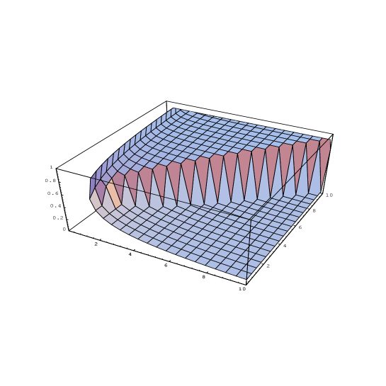
FIG. 3.:

Plot of the bulk densities $m_{>}$, $m_{<}$ in phases A and B in the region accessible by the 2-d representation.                                          $\kappa_{+}(\alpha,\gamma)$                                                                                                        $\kappa_{+}(\beta,\delta)$           $m_{>},m_{<}$

Unlike the quantities $m_{>}$ and $m_{<}$ the coefficients $c_{<}$ and $c_{>}$ of the exponentials are not universal in the sense that they are not only functions of $\kappa_{+}(\alpha,\gamma)$ and $\kappa_{+}(\beta,\delta)$. However, the correlation length $|\zeta|$ in the exponential can be expressed as

$$\exp\left(\frac{1}{\zeta}\right)=\frac{\kappa_{+}(\alpha,\gamma)}{\kappa_{+}(\beta,\delta)}\left(\frac{1+\kappa_{+}(\beta,\delta)}{1+\kappa_{+}(\alpha,\gamma)}\right)^{2}\ .$$ (166)

This shows that the correlation length $|\zeta|$ diverges when $\kappa_{+}(\alpha,\gamma)$ and $\kappa_{+}(\beta,\delta)$ approach the coexistence line: $\zeta\rightarrow\infty$ when approaching the coexistence line from phase $A$, and $\zeta\rightarrow-\infty$ from phase $B$. It is interesting to compare (116) with (166). Surprisingly enough, for phases $A_{I}$ and $B_{I}$ the $0=\gamma=\delta=q$ correlation length has precisely the expression (166). This ceases to be the case for phases $A_{II}$ and $B_{II}$. We would like to stress that although the mean-field values (164) are exact, the correlation length $\zeta$ given by (166) cannot be obtained in the mean-field approximation.

The two-point function can be evaluated in way analogous to the case of the one-point function discussed above. After some straightforward computations we obtain

$$\langle\tau_{j}\tau_{k}\rangle=\Omega^{\prime}\left(\omega_{3}+\omega_{4}\exp\left(\frac{L-k}{\zeta}\right)+\omega_{5}\exp\left(\frac{L-j-1}{\zeta}\right)+\omega_{6}\exp\left(\frac{L-2}{\zeta}\right)\right)\ ,$$ (167)

where

$$\Omega^{\prime} = \frac{1}{\lambda_{+}^{2}[(\beta+\delta)b_{2}-(\alpha+\gamma)a_{2}\exp\left(\frac{L}{\zeta}\right)]}\ ,$$ (168)

$$\omega_{3} = (\beta+\delta)b_{2}\left(\frac{\alpha+\delta+\alpha a_{2}}{\alpha\beta-\gamma\delta}\right)^{2}\ ,$$ (169)

$$\omega_{4} = -a_{2}b_{2}\ \frac{\alpha+\delta+\alpha a_{2}}{\alpha\beta-\gamma\delta}\ ,$$ (170)

$$\omega_{5} = -a_{2}b_{2}\ \frac{\alpha+\delta+\delta b_{2}}{\alpha\beta-\gamma\delta}\ ,$$ (171)

$$\omega_{6} = -(\alpha+\gamma)a_{2}\left(\frac{\alpha+\delta+\delta b_{2}}{\alpha\beta-\gamma\delta}\right)^{2}\ .$$ (172)

Again we have to distinguish between two cases

• $\zeta<0$ (low-density phase): The connected two-point function in the large $L$ limit is given by

  $$\langle\tau_{j}\tau_{k}\rangle-\langle\tau_{j}\rangle\langle\tau_{k}\rangle=c_{<}(m_{>}-m_{<})\exp\left(\frac{L-j}{\zeta}\right)-c_{<}^{2}\exp\left(\frac{2L-j-k}{\zeta}\right)\ ,$$ (173)

  It is different from zero only very close to the right boundary, from where it decays exponentially.

• $\zeta>0$ (high-density phase) :

  $$\langle\tau_{j}\tau_{k}\rangle-\langle\tau_{j}\rangle\langle\tau_{k}\rangle=c_{>}(m_{<}-m_{>})\exp\left(\frac{-k+1}{\zeta}\right)-c_{>}^{2}\exp\left(\frac{-j-k+2}{\zeta}\right)\ ,$$ (174)

  Thus the connected two-point function in phase A is different from zero only very close to the left boundary, where it exhibits an exponential behaviour.

X Correlation Functions on the Coexistence Line ($\lambda_{+}=\lambda_{-}$)

For the case $\alpha=\beta$, $\gamma=\delta$ we have $\kappa_{+}(\alpha,\gamma)=\kappa_{+}(\beta,\delta)>1$ with

$$\kappa_{+}(\alpha,\gamma)=\sqrt{\frac{p}{q}}$$ (175)

and are thus on the phase boundary between the high-density phase $A$ and the low-density phase $B$. Here we have taken into account the constraint (130) for the 2-d representation, which can be solved with the result

$$\gamma=-p+(\alpha+q)\sqrt{\frac{p}{q}}\ .$$ (176)

The matrix elements of the matrices $A$ and $B$ in (138) are found to be

$$a_{2}=b_{2}=-if_{1}=\sqrt{\frac{p}{q}}-1-\alpha\frac{\sqrt{q}+\sqrt{p}}{q\sqrt{p}}\ ,$$ (177)

which leads to the following form for the matrix $C$

$$C=\frac{1}{\alpha-\gamma}\left((2+a_{2})I+a_{2}P\right)\ ,\ P=\left(\matrix{-1&i\cr i&1\cr}\right)\ .$$ (178)

The matrix $P$ has the property $P^{2}=0$, which is important for carrying out the calculations below. Using the fact that $P^{2}=0$ it is easy to show that

$$C^{k}=\frac{(2+a_{2})^{k-1}}{(\alpha-\gamma)^{k}}\left(\matrix{2+(1-k)a_{2}&ika_{2}\cr ika_{2}&2+(1+k)a_{2}\cr}\right)\ ,$$ (179)

which implies that the normalization is given by

$$\langle W|C^{L}|V\rangle=\frac{(2+a_{2})^{L-1}}{(\alpha-\gamma)^{L}}(2+(1-L)a_{2})\ .$$ (180)

Using (180) we can easily evaluate the current

$$J=\left(\frac{\alpha-\gamma}{2+a_{2}}\right)\left(\frac{2+(2-L)a_{2}}{2+(1-L)a_{2}}\right).$$ (181)

In the thermodynamic limit this simplifies to

$$J=\frac{\alpha-\gamma}{2+a_{2}}=\sqrt{pq}\frac{1-{\cal Q}}{1+{\cal Q}}\ ,\quad{\cal Q}={\sqrt{\frac{q}{p}}}\equiv\frac{1}{\kappa_{+}(\alpha,\gamma)}\ ,$$ (182)

which in turn can be shown to be equal to (120).

The density profile is

$$\langle\tau_{j}\rangle=\frac{(\alpha+\gamma)(2+a_{2}(2-L))+a_{2}^{2}(\gamma-L\alpha)}{(\alpha+\gamma)(2+a_{2})(2+(1-L)a_{2})}+\frac{(\alpha-\gamma)a_{2}^{2}}{(\alpha+\gamma)(2+a_{2})(2+(1-L)a_{2})}j\ .$$ (183)

In the thermodynamic limit $j,L\rightarrow\infty$ $\frac{j}{L}=x$ fixed, this turns into

$$\langle\tau_{Lx}\rangle = \frac{{\cal Q}}{1+{\cal Q}}+\frac{{1-\cal Q}}{1+{\cal Q}}x\ .$$ (184)

This means that for $p>q$ the density increases linearly from $\frac{{\cal Q}}{1+{\cal Q}}$ at the left end of the chain to $\frac{1}{1+{\cal Q}}$, whereas for $q>p$ is decreases linearly from $\frac{{\cal Q}}{1+{\cal Q}}$ to $\frac{1}{1+{\cal Q}}$. Clearly the profile is symmetric under simulataneous interchange of $p$ and $q$ and left and right as it should be. The most remarkable feature of the profile (184) is the fact that it is independent of the injection/extraction rate $\alpha$. The only relevant parameter is the ratio $\frac{p}{q}$ of the diffusion rates to the right and to the left. This fact is probably a feature of the particular representation we work with since in the completely asymmetric case the current and density profile on the coexistence line are dependent on the boundary condition $\alpha$ (see (111)), and we expect that in general the current and density profile in the partially asymmetric case will depend on the boundary conditions as well.

The two-point function can be determined by using (179) in (88) and is found to be of the form

$$\langle\tau_{j}\tau_{k}\rangle=\omega_{7}+\omega_{8}j+\omega_{9}k\ ,$$ (185)

where

$$\omega_{7} = \frac{(\alpha+\gamma)^{2}[2+a_{2}(3-L)+a_{2}^{2}]+2a_{2}^{2}[\gamma^{2}-L\alpha(\alpha+\gamma)]+a_{2}^{3}[\gamma^{2}-L\alpha^{2}]}{(2+a_{2})^{2}(2+a_{2}(1-L))(\alpha+\gamma)^{2}}\ ,$$ (186)

$$\omega_{8} = \frac{(\alpha-\gamma)a_{2}^{2}(\alpha+\gamma+\gamma a_{2})}{(2+a_{2})^{2}(2+a_{2}(1-L))(\alpha+\gamma)^{2}}\ ,$$ (187)

$$\omega_{9} = \frac{(\alpha-\gamma)a_{2}^{2}(\alpha+\gamma+\alpha a_{2})}{(2+a_{2})^{2}(2+a_{2}(1-L))(\alpha+\gamma)^{2}}\ .$$ (188)

In the limit $j,k,L\rightarrow\infty$ with $\frac{j}{L}=x$ and $\frac{k}{L}=y$ fixed this simplifies essentially

$$\langle\tau_{Lx}\tau_{Ly}\rangle=\left(\frac{{\cal Q}}{1+{\cal Q}}\right)^{2}+\frac{1-{\cal Q}}{\left(1+{\cal Q}\right)^{2}}x+\frac{{\cal Q}(1-{\cal Q})}{\left(1+{\cal Q}\right)^{2}}y\ .$$ (189)

Using (184) we finally arrive at the following result for the connected two-point function

$$\langle\tau_{Lx}\tau_{Ly}\rangle-\langle\tau_{Lx}\rangle\langle\tau_{Ly}\rangle=\left(\frac{1-{\cal Q}}{1+{\cal Q}}\right)^{2}x(1-y)\ .$$ (190)

Like the density profile the connected two-point function is independent of $\alpha$. It takes its maximal value $\left(\frac{1-{\cal Q}}{2(1+{\cal Q})}\right)^{2}$ in the middle of the chain, and decreases to zero at both boundaries. It is interesting to note that a similar expression for the connected two-point function was obtained for the completely asymmetric (particles hop only to the right) deterministic exclusion model with stochastic boundary effects [24].

XI Summary and Conclusion

In this paper we have first presented the Fock representations of the quadratic algebra. The representations can be either infinite-dimensional or finite-dimensional. Each finite-dimensional representation is characterized by a constraint on the seven parameters of the algebra. The matrix elements of the two generators of the algebra are given by recurrence relations. Only in the cases where these relations can be solved in a simple way the corresponding Fock-representation is useful for studying the physical problem of partially asymmetric diffusion with open boundaries. Quadratic algebras with more than two generators, which are relevant for many-state problems, will be presented elsewhere. The structure of the associative algebra is different for these cases [28]. The boundary conditions define representations of a different type as compared to the Fock representations considered here.

The quadratic algebra appears in the DEHP Ansatz for the steady-state probability distributions of one-dimensional reaction diffusion problems with two-body rates and injection and extraction of particles at the ends of the chain. As shown in section V and also in [3, 25], the quadratic algebra appears also for some more general reaction-diffusion processes. As also shown in the present work, if one considers three-body rates, cubic algebras occur. We have not studied the representation theory for that case.

We have used the 2-d representation of the quadratic algebra to compute the density profile and correlation functions. Both have a special dependence on the coordinates (see (174) and (173)). The parameter dependence is also peculiar. Certain quantities like the density around the middle of the chain or the correlation length depend on the parameters $\alpha,\beta,\gamma,\delta,p,q$ only through two functions $\kappa_{+}(\alpha,\gamma)$ and $\kappa_{+}(\beta,\delta)$ defined in the text. Our results and those of [11, 12, 13] suggest that the density in the bulk is given by the mean-field prediction in the thermodynamic limit. Again from our results and those of [11, 12, 13] it looks like the correlation lengths again are “universal” (they depend only on $\kappa_{+}(\alpha,\gamma)$ and $\kappa_{+}(\beta,\delta)$) in regions $A_{I}$ and $B_{I}$ of the phase diagram.

By means of (71) our results (173), (174) and (190) for the connected two-point functions can be directly translated to the XXZ quantum-spin chain (65) with non-diagonal boundary terms. This yields new and nontrivial results for correlators in the XXZ chain with boundaries. We have not considered the problem of time-dependent correlation functions. Some recent numerical results of Bilstein [26] can give a hint in this direction. He studied the finite-size scaling bahaviour of the energy gaps of the quantum hamiltonian. It turns out that in the low- and high-density phases the system is massive. In phase $C$ (see Fig.2) the system is massless. Both real and imaginary parts of the energy gaps vanish like $L^{-\frac{3}{2}}$, where $L$ is the size of the system. The coexistence line is also massless but features a less simple length dependence.

Finally, as a by-product of our work on the DEHP construction, we have given a simple way to construct irreducible representations of the $U_{q}(SU(2))$ quantum group.

Acknowledgements

We are grateful to A. Berkovich for a useful suggestion and to K. Krebs, M. Scheunert, H.Z. Simon and G. Schütz for reading the manuscript and discussions. We thank A. Dzhumadildaev for pointing out refererences [16] and [28] to us.

Appendix A

We would like to show that in the Fock representation of the quadratic algebra (2) the matrices $A$ and $B$ can be written in tridiagonal form. This is a property of the Fock representation only, and is independent of the parameters $x_{i}$. Instead of presenting the general proof, we give two examples which will help the reader to see the mechanism behind the proof. We start with the 2-d representation. We choose $|V\rangle=\pmatrix{1\cr 0}$ and take $\langle W|=\pmatrix{w_{1},&w_{2}}$ with $w_{1}\neq 0$ such that $\langle W|V\rangle\neq 0$. We then perform a similarity transformation

$$S=\left(\matrix{1&\alpha\cr 0&1}\right)\ ,\ S|V\rangle=|V\rangle\ ,\ \langle W|S^{-1}=\pmatrix{w_{1},&-\alpha w_{1}+w_{2}}\ ,$$ (191)

where we choose $\alpha=\frac{w_{2}}{w_{1}}$ and $w_{1}=1$, which results in $\langle W|=\pmatrix{1,&0}$ and $\langle W|V\rangle=1$. In this basis $A$ and $B$ now must be of the form

$$A=\left(\matrix{0&a_{12}\cr 0&a_{22}\cr}\right)\ ,\ B=\left(\matrix{0&0\cr b_{21}&b_{22}\cr}\right)\ .$$ (192)

We now perform another similarity transformation

$$S=\left(\matrix{1&0\cr 0&\beta\cr}\right)\ ,\ \langle W|S^{-1}=\langle W|\ ,\ S|V\rangle=|V\rangle$$ (193)

where we choose $\beta^{2}=\frac{a_{12}}{b_{21}}$ and find two equivalent representations

$$A=\left(\matrix{0&\pm\sqrt{a_{12}b_{21}}\cr 0&a_{22}\cr}\right)\ ,\ B=\left(\matrix{0&0\cr\pm\sqrt{a_{12}b_{21}}&b_{22}\cr}\right)\ .$$ (194)

Here we have assumed that both $a_{12}$ and $b_{21}$ are different from zero. One can show that if $a_{12}=0$ or $b_{21}=0$ the algebra (2) yields the condition $x_{7}=0$, which corresponds to the 1-d representation and thus the 2-d representation is not interesting. Renaming the entries of $A$ and $B$ we arrive at

$$A=\left(\matrix{0&f_{1}\cr 0&a_{2}\cr}\right)\ ,\ B=\left(\matrix{0&0\cr f_{1}&b_{2}\cr}\right)\ .$$ (195)

Let us now consider the 3-d representation. We can repeat the similarity transformations from the 2-d case to bring $A$ and $B$ to the form ($f_{1}^{\prime}\neq 0$)

$$A=\left(\matrix{0&f_{1}^{\prime}&g_{1}^{\prime}\cr 0&a_{22}^{\prime}&a_{23}^{\prime}\cr 0&a_{32}^{\prime}&a_{33}^{\prime}\cr}\right)\ ,\ B=\left(\matrix{0&0&0\cr f_{1}^{\prime}&b_{22}^{\prime}&b_{23}^{\prime}\cr g_{1}^{\prime}&b_{32}^{\prime}&b_{33}^{\prime}\cr}\right)\ ,$$ (196)

where $|V\rangle=\pmatrix{1\cr 0\cr 0\cr}$ and $\langle W|=\pmatrix{1,&0,&0}$. Taking the further similarity transformation

$$S=\left(\matrix{1&0&0\cr 0&\cos(\theta)&\sin(\theta)\cr 0&-\sin(\theta)&\cos(\theta)\cr}\right)\ ,\quad\tan(\theta)=\frac{g_{1}^{\prime}}{f_{1}^{\prime}}$$ (197)

we get

$$A=\left(\matrix{0&f_{1}&0\cr 0&a_{22}&a_{23}\cr 0&a_{32}&a_{33}\cr}\right)\ ,\ B=\left(\matrix{0&0&0\cr f_{1}&b_{22}&b_{23}\cr 0&b_{32}&b_{33}\cr}\right)\ .$$ (198)

Finally, by means of a diagonal similarity transformation we can bring $A$ and $B$ to the form

$$A=\left(\matrix{0&f_{1}&0\cr 0&a_{2}&f_{2}\cr 0&h_{2}&a_{3}\cr}\right)\ ,\ B=\left(\matrix{0&0&0\cr f_{1}&b_{2}&k_{2}\cr 0&f_{2}&b_{3}\cr}\right)\ .$$ (199)

This procedure can be generalized to any dimension of the representation. We can thus search for representations of the quadratic algebra starting with the tridiagonal form

$$\tilde{A}=\left(\matrix{0&f_{1}&0&0&0&0&0\ldots\cr 0&a_{2}&f_{2}&0&0&0&0\ldots\cr 0&h_{2}&a_{3}&f_{3}&0&0&0\ldots\cr 0&0&h_{3}&a_{4}&f_{4}&0&0\ldots\cr\ldots&&&&\ldots&&\cr}\right)$$ (200)

$$\tilde{B}=\left(\matrix{0&0&0&0&0&0&0\ldots\cr f_{1}&b_{2}&k_{2}&0&0&0&0\ldots\cr 0&f_{2}&b_{3}&k_{3}&0&0&0\ldots\cr 0&0&f_{3}&b_{4}&k_{4}&0&0\ldots\cr\ldots&&&&\ldots&&\cr}\right)\ .$$ (201)

Appendix B

In this appendix we discuss a generalization of the DEHP-formalism to chemical processes of the types given in (51) that incorporate three neighbouring sites. By construction all models discussed above are contained in the present formulation. From a physical point of view this generalization is quite interesting. For purely diffusive processes it allows us e.g. to let particles hop to the next-nearest neighbour site if the nearest neighbour site is unoccupied. In the corresponding traffic-flow picture this corresponds to letting cars move faster or slower depending on whether the road ahead is free for a long or a short distance.

We consider a master-equation of the form

$$0=\frac{\partial P}{\partial t} = -\sum_{k=1}^{L-2}\sum_{\gamma_{k},\gamma_{k+1},\gamma_{k+2}}\left(H_{k,k+1,k+2}\right)_{\tau_{k},\tau_{k+1},\tau_{k+2}}^{\gamma_{k},\gamma_{k+1},\gamma_{k+2}}P_{L}(\tau_{1},\tau_{2}\ldots\tau_{k-1},\gamma_{k},\gamma_{k+1},\gamma_{k+2},\tau_{k+3}\ldots\tau_{L})$$ (203)

$$-\sum_{\gamma_{1}\gamma_{2}}(h_{12})_{\tau_{1}\tau_{2}}^{\gamma_{1}\gamma_{2}}P_{L}(\gamma_{1}\gamma_{2}\tau_{3}\ldots\tau_{L})-\sum_{\gamma_{L-1}\gamma_{L}}(h_{L-1L})_{\tau_{L-1}\tau_{L}}^{\gamma_{L-1}\gamma_{L}}P_{L}(\tau_{1}\ldots\tau_{L-2}\gamma_{L-1}\gamma_{L})\ ,$$

where

$$\left(H_{k,k+1,k+2}\right)_{\tau_{k},\tau_{k+1},\tau_{k+2}}^{\gamma_{k},\gamma_{k+1},\gamma_{k+2}}=\Bigg{\{}\matrix{\sum^{\prime}_{\beta_{k},\beta_{k+1},\beta_{k+2}}\Gamma_{\beta_{k},\beta_{k+1},\beta_{k+2}}^{\gamma_{k},\gamma_{k+1},\gamma_{k+2}}\qquad\gamma_{j}=\tau_{j}\ ,\ j=k,k+1,k+2\cr-\Gamma_{\tau_{k},\tau_{k+1},\tau_{k+2}}^{\gamma_{k},\gamma_{k+1},\gamma_{k+2}}\qquad{\rm else\ .}\cr}$$ (204)

Here $\Gamma^{\alpha\beta\gamma}_{\alpha^{\prime}\beta^{\prime}\gamma^{\prime}}$ is the probability per unit time that the configuration $(\alpha\beta\gamma)$ on three neighbouring sites changes to the configuration $(\alpha^{\prime}\beta^{\prime}\gamma^{\prime})$. Following the analysis in section $1$ above we demand for the probability distribution in the bulk that

$$-\sum_{\gamma_{k},\gamma_{k+1},\gamma_{k+2}} \left(H_{k,k+1,k+2}\right)_{\tau_{k},\tau_{k+1},\tau_{k+2}}^{\gamma_{k},\gamma_{k+1},\gamma_{k+2}}P_{L}(\tau_{1},\tau_{2}\ldots\tau_{k-1},\gamma_{k},\gamma_{k+1},\gamma_{k+2},\tau_{k+3}\ldots\tau_{L})$$ (205)

$$= x_{\tau_{k}}P_{L-1}(\tau_{1}\ldots\tau_{k-1}\tau_{k+1}\ldots\tau_{L})-x_{\tau_{k+1}}P_{L-1}(\tau_{1}\ldots\tau_{k}\tau_{k+2}\ldots\tau_{L})$$ (209)

$$+y_{\tau_{k}}P_{L-1}(\tau_{1}\ldots\tau_{k-1}\tau_{k+1}\ldots\tau_{L})-y_{\tau_{k+2}}P_{L-1}(\tau_{1}\ldots\tau_{k+1}\tau_{k+3}\ldots\tau_{L})$$

$$+z_{\tau_{k+1}}P_{L-1}(\tau_{1}\ldots\tau_{k}\tau_{k+2}\ldots\tau_{L})-z_{\tau_{k+2}}P_{L-1}(\tau_{1}\ldots\tau_{k+1}\tau_{k+3}\ldots\tau_{L})$$

$$+t_{\tau_{k}\tau_{k+1}}P_{L-2}(\tau_{1}\ldots\tau_{k-1}\tau_{k+2}\ldots\tau_{L})-t_{\tau_{k+1}\tau_{k+2}}P_{L-2}(\tau_{1}\ldots\tau_{k}\tau_{k+3}\ldots\tau_{L}).$$

This ensures that there will be no contribution from the bulk to the r.h.s. of (203), as all terms will cancel when summed over $(k,k+1,k+2)$. As compared to (77) it is now possible to include terms containing probability distributions $P_{L-2}$ with two fewer particles. The r.h.s. of (209) can be simplified by introducing the notation

$$\mu_{b_{k}}=x_{b_{k}}+y_{b_{k}}\ ,\ \nu_{b_{k}}=z_{b_{k}}-x_{b_{k}}\ ,\ \lambda_{b_{k}}=-\mu_{b_{k}}-\nu_{b_{k}}\ .$$ (210)

From the boundaries we get the conditions that

$$\sum_{\gamma_{1}\gamma_{2}}(h_{12})_{\tau_{1}\tau_{2}}^{\gamma_{1}\gamma_{2}}P_{L}(\gamma_{1}\gamma_{2}\tau_{3}\ldots\tau_{L})=t_{\tau_{1}\tau_{2}}P_{L-2}(\tau_{3}\ldots\tau_{L})+\mu_{\tau_{1}}P_{L-1}(\tau_{2}\ldots\tau_{L})$$ (211)

$$\hskip 113.81102pt-\lambda_{\tau_{2}}P_{L-1}(\tau_{1}\tau_{3}\ldots\tau_{L})$$ (212)

$$\sum_{\gamma_{L-1}\gamma_{L}}(h_{L-1L})_{\tau_{L-1}\tau_{L}}^{\gamma_{L-1}\gamma_{L}}P_{L}(\tau_{1}\ldots\tau_{L-2}\gamma_{L-1}\gamma_{L})=$$ (213)

$$-t_{\tau_{L-1}\tau_{L}}P_{L-2}(\tau_{1}\ldots\tau_{L-2})-\mu_{\tau_{L-1}}P_{L-1}(\tau_{1}\ldots\tau_{L-2}\tau_{L})+\lambda_{\tau_{L}}P_{L-1}(\tau_{1}\ldots\tau_{L-1})\ .$$ (214)

Here we have allowed for arbitrary processes of the type introduced in (51) to occur on the first two and last two sites of the lattice. Putting everything together we arrive at the following algebra

$$-{\cal H}\pmatrix{D^{3}\cr D^{2}E\cr DED\cr ED^{2}\cr DE^{2}\cr EDE\cr E^{2}D\cr E^{3}\cr}=\pmatrix{0\cr\mu_{1}DE+\nu_{1}DE+\lambda_{0}D^{2}+t_{11}E-t_{10}D\cr\mu_{1}ED+\nu_{0}D^{2}+\lambda_{1}DE+t_{10}D-t_{01}D\cr\mu_{0}D^{2}+\nu_{1}ED+\lambda_{1}ED+t_{01}D-t_{11}E\cr\mu_{1}E^{2}+\nu_{0}DE+\lambda_{0}DE+t_{10}E-t_{00}D\cr\mu_{0}DE+\nu_{1}E^{2}+\lambda_{0}ED+t_{01}E-t_{10}E\cr\mu_{0}ED+\nu_{0}ED+\lambda_{1}E^{2}+t_{00}D-t_{01}E\cr 0\cr}\ ,$$ (215)

where

$${\cal H}=\left(\matrix{H^{111}_{111}&\Gamma^{110}_{111}&\Gamma^{101}_{111}&\Gamma^{011}_{111}&\Gamma^{100}_{111}&\Gamma^{010}_{111}&\Gamma^{001}_{111}&\Gamma^{000}_{111}\cr\Gamma^{111}_{110}&H^{110}_{110}&\Gamma^{101}_{110}&\Gamma^{011}_{110}&\Gamma^{100}_{110}&\Gamma^{010}_{110}&\Gamma^{001}_{110}&\Gamma^{000}_{110}\cr\Gamma^{111}_{101}&\Gamma^{110}_{101}&H^{101}_{101}&\Gamma^{011}_{101}&\Gamma^{100}_{101}&\Gamma^{010}_{101}&\Gamma^{001}_{101}&\Gamma^{000}_{101}\cr\Gamma^{111}_{011}&\Gamma^{110}_{011}&\Gamma^{101}_{011}&H^{011}_{011}&\Gamma^{100}_{011}&\Gamma^{010}_{011}&\Gamma^{001}_{011}&\Gamma^{000}_{011}\cr\Gamma^{111}_{100}&\Gamma^{110}_{100}&\Gamma^{101}_{100}&\Gamma^{011}_{100}&H^{100}_{100}&\Gamma^{010}_{100}&\Gamma^{001}_{100}&\Gamma^{000}_{100}\cr\Gamma^{111}_{010}&\Gamma^{110}_{010}&\Gamma^{101}_{010}&\Gamma^{011}_{010}&\Gamma^{100}_{010}&H^{010}_{010}&\Gamma^{001}_{010}&\Gamma^{000}_{010}\cr\Gamma^{111}_{001}&\Gamma^{110}_{001}&\Gamma^{101}_{001}&\Gamma^{011}_{001}&\Gamma^{100}_{001}&\Gamma^{010}_{001}&H^{001}_{001}&\Gamma^{000}_{001}\cr\Gamma^{111}_{000}&\Gamma^{110}_{000}&\Gamma^{101}_{000}&\Gamma^{011}_{000}&\Gamma^{100}_{000}&\Gamma^{010}_{000}&\Gamma^{001}_{000}&H^{000}_{000}\cr}\right)\ .$$ (216)

It is clear that only seven of the eight equations in (216) are independent. The boundary conditions are rewritten as

$$\sum_{\gamma_{1}\gamma_{2}}(h_{12})_{\tau_{1}\tau_{2}}^{\gamma_{1}\gamma_{2}}\langle W|[\gamma_{1}D+(1-\gamma_{1})E][\gamma_{2}D+(1-\gamma_{2})E]$$ (217)

$$\qquad=\langle W|\bigg{[}(t_{\tau_{1}\tau_{2}}+\mu_{\tau_{1}}[\tau_{2}D+(1-\tau_{2})E]-\lambda_{\tau_{2}}[\tau_{1}D+(1-\tau_{1})E]\bigg{]}$$ (218)

$$\sum_{\gamma_{L-1}\gamma_{L}}(h_{L-1L})_{\tau_{L-1}\tau_{L}}^{\gamma_{L-1}\gamma_{L}}[\gamma_{L-1}D+(1-\gamma_{L-1})E][\gamma_{L}D+(1-\gamma_{L})E]|V\rangle$$ (219)

$$\qquad=\bigg{[}-t_{\tau_{L-1}\tau_{L}}+\lambda_{\tau_{L}}[\tau_{L-1}D+(1-\tau_{L-1})E]-\mu_{\tau_{L-1}}[\tau_{L}D+(1-\tau_{L})E]\bigg{]}|V\rangle\ .$$ (220)

Note that the algebra (216) is cubic and that the conditions at the boundaries are quadratic in $D$ and $E$.

If we constrain ourselves to diffusion processes only, the system (216) decouples into two sets of respectively two independent equations

$${\cal H}_{1}\pmatrix{D^{2}E\cr DED\cr ED^{2}\cr} = \pmatrix{-\lambda_{1}DE+\lambda_{0}D^{2}+t_{11}E-t_{10}D\cr\mu_{1}ED+\nu_{0}D^{2}+\lambda_{1}DE+t_{10}D-t_{01}D\cr}\ ,$$ (221)

$${\cal H}_{2}\pmatrix{DE^{2}\cr EDE\cr E^{2}D\cr} = \pmatrix{\mu_{1}E^{2}-\mu_{0}DE+t_{10}E-t_{00}D\cr\mu_{0}DE+\nu_{1}E^{2}+\lambda_{0}ED+t_{01}E-t_{10}E\cr}\ ,$$ (222)

where

$${\cal H}_{1} = \left(\matrix{-\Gamma^{110}_{101}-\Gamma^{110}_{011}&\Gamma^{101}_{110}&\Gamma^{011}_{110}\cr\Gamma^{110}_{101}&-\Gamma^{101}_{110}-\Gamma^{101}_{011}&\Gamma^{011}_{101}\cr}\right)$$ (223)

$${\cal H}_{2} = \left(\matrix{-\Gamma^{100}_{010}-\Gamma^{100}_{001}&\Gamma^{010}_{100}&\Gamma^{001}_{100}\cr\Gamma^{100}_{010}&-\Gamma^{010}_{100}-\Gamma^{010}_{001}&\Gamma^{001}_{010}\cr}\right)\ .$$ (224)

In order to demonstrate that there exist solutions to these equations we will prove the existence of a one-dimensional representation for the special choice of boundary conditions

$$(h_{1})^{00}_{11} = -\alpha=-(h_{1})^{00}_{00}$$ (225)

$$(h_{L})^{11}_{00} = -\beta=-(h_{L})^{11}_{11}\ ,$$ (226)

which correspond to injection of particles at sites $1$ and $2$ with probability $\alpha$ if both sites are empty, and extraction of particles at sites $L-1$ and $L$ with probability $\beta$ if both sites are occupied. The one-dimensional representation exists if $D=E=1$ and

$$\alpha = \beta=\Gamma^{110}_{101}+\Gamma^{110}_{011}-\Gamma^{101}_{110}-\Gamma^{101}_{110}=\Gamma^{100}_{010}+\Gamma^{100}_{001}-\Gamma^{010}_{100}-\Gamma^{001}_{100}\ ,$$ (227)

$$\Gamma^{110}_{101}+\Gamma^{011}_{101} = \Gamma^{101}_{011}+\Gamma^{101}_{110}\ ,\quad\Gamma^{100}_{010}+\Gamma^{001}_{010}=\Gamma^{010}_{001}+\Gamma^{010}_{100}\ .$$ (228)

The corresponding probability distribution is trivial

$$P_{L}(\tau_{1}\ldots\tau_{L})=\frac{1}{2^{L}}\ ,$$ (229)

which means that all configurations are equally represented. Although the existence of the 1-d representations is a nontrivial fact, the corresponding physics is not particularly interesting. It would be very interesting to construct finite or infinite dimensional representation and use them to compute currents, density profiles etc.

Appendix C

In this appendix we consider the special case $0=\gamma=\delta$ and $\alpha=\beta=p-q$ of the algebra (81). As was shown in (96) the quadratic algebra reduces to a Q-osciallator algebra. We introduce the following notation for Q-numbers

$$\{n\}=\frac{1-Q^{n}}{1-Q}\ ,$$ (230)

and Q-binomials

$${\cal C}^{p}_{n}(Q)=\frac{\{n\}\{n-1\}\dots\{2\}}{\{n-p\}\{n-p-1\}\dots\{2\}\{p\}\{p-1\}\dots\{2\}}=\frac{\prod_{r=1}^{n}(1-Q^{r})}{\prod_{s=1}^{p}(1-Q^{s})\prod_{t=1}^{n-p}(1-Q^{t})}\ .$$ (231)

In order to compute the current or correlation functions a convenient representation of $C^{N}=(D+E)^{N}$ is required. In terms of $a$ and $a^{\dagger}$ we find

$$C^{N}=\frac{1}{p^{N}}\left(\frac{2}{1-Q}+\frac{a+a^{\dagger}}{\sqrt{1-Q}}\right)^{N}=\left(\frac{2}{p-q}\right)^{N}\sum_{j=0}^{N}{\cal C}^{j}_{N}(1)(a+a^{\dagger})^{j}\left(\frac{\sqrt{1-Q}}{2}\right)^{j}\ .$$ (232)

In order to evaluate e.g. the normalization $\langle 0|C^{L}|0\rangle$ it is convenient to decompose powers of $a+a^{\dagger}$ into normal-ordered expressions defined via

$$:(a+a^{\dagger})^{n}:=\sum_{p=0}^{n}{\cal C}^{p}_{n}(Q){a^{\dagger}}^{p}a^{n-p}\ .$$ (233)

The decomposition is of the form

$$(a+a^{\dagger})^{n}=\sum_{m=0}^{\left[\frac{n}{2}\right]}M^{(m)}_{n}:(a+a^{\dagger})^{n-2m}:\ .$$ (234)

Using the identity

$$(a+a^{\dagger})\ :(a+a^{\dagger})^{n}:=:(a+a^{\dagger})^{n+1}:+\{n\}:(a+a^{\dagger})^{n-1}:\ ,$$ (235)

one readily obtains recursive expressions for $M^{(k)}_{n}$

$$M^{(0)}_{n}=1\ ,\ M^{(1)}_{n}=\sum_{l=1}^{n-1}\{l\}\ ,\ M^{(2)}_{n}=\sum_{l=1}^{n-3}\{l\}M^{(1)}_{l+2}\ ,\ M^{(3)}_{n}=\sum_{l=1}^{n-5}\{l\}M^{(2)}_{l+4}\ ,\ldots$$ (236)

We first note the result for the cases $Q=1$ (no deformation) and $Q=0$

$$M^{(m)}_{n}\bigg{|}_{Q=1} = \pmatrix{n\cr 2m}\prod_{k=0}^{m-1}(2k+1)=\frac{n!}{(n-2m)!\ (2m)!!}\ ,$$ (237)

$$M^{(m)}_{n}\bigg{|}_{Q=0} = \pmatrix{n-1\cr m}-\pmatrix{n-1\cr m-2}\ .$$ (238)

After some tedious computations we find for arbitrary $Q$

$$M^{(1)}_{n} = \frac{n-\{n\}}{1-Q}\ ,$$ (239)

$$M^{(2)}_{n} = \frac{1}{(1-Q)^{2}}\left[n\left(\frac{n-1}{2}-\{n-2\}\right)-\{n\}\left(\frac{\{n-3\}}{\{2\}}-\{n-3\}\right)\right]\ .$$ (240)

We did not succeed in obtaining a closed form for $M^{(k)}_{n}$ for general $k$. The difficulty can be traced back to the recurrence relation (236) which although it is written entirely in terms of $Q$-numbers does not have $Q$-number solutions (the sum of $Q$-numbers is not a $Q$-number).

Appendix D

In this appendix we would like to show that the DEHP-Ansatz gives a new way to construct irreducible representations of the quantum group $U_{q}(SU(2))$ and that the quantum plane appears in a natural way. We consider the special case $0=\xi=\eta$, $\lambda=q/p$, $z_{2}={p}/({p-q})$ of (81). The boundary conditions are taken such that $0=\gamma=\delta$, then the limit $\alpha\rightarrow 0$, $\beta\rightarrow 0$ is performed. For $0=\alpha=\beta=\gamma=\delta$ the XXZ quantum spin hamiltonian (65) corresponding to the diffusion process is invariant under the quantum algebra $U_{q}(SU(2))$ ([17, 6] and references therein). The stationary state (72) is no more unique since the ground state of the ferromagnetic chain is $L+1$-times degenerate corresponding to a multiplet of $sl_{q}(2)$. As the boundary conditions (81) become ill-defined in the case $0=\alpha=\beta=\gamma=\delta$ we carefully take the limit $\alpha\rightarrow 0$, $\beta\rightarrow 0$ with $0=\gamma=\delta$ as follows

$$\alpha = \frac{\varepsilon}{e},\ \beta=\frac{\varepsilon}{d},\ {\bar{D}}=\varepsilon D,\ {\bar{E}}=\varepsilon E,$$ (241)

$$\langle W|{\bar{E}} = e\langle W|,\ {\bar{D}}|V\rangle=d|V\rangle,\$$ (242)

where ${\bar{D}}$ and ${\bar{E}}$ are seen to obey the quantum plane equation

$${\bar{D}}{\bar{E}}={\cal Q}^{2}{\bar{E}}{\bar{D}}\ ,\ {\cal Q}^{2}=\frac{q}{p}\ .$$ (243)

The quantum-mechanical state corresponding to the stationary state of the diffusion process is obtained by applying (54)

$$|0\rangle=\frac{1}{{\cal N}}\sum_{k=0}^{L}d^{L-k}e^{k}\sum_{i_{1}<i_{2}<\ldots<i_{k}}{\cal Q}^{2(i_{1}+i_{2}+\ldots+i_{k}-\frac{k+k^{2}}{2})}\prod_{l=1}^{k}\sigma^{-}_{i_{l}}|\uparrow\uparrow\ldots\uparrow\rangle,$$ (244)

where $\frac{1}{{\cal N}}$ is a normalization factor. Note that $|0\rangle$ is a linear combination of $L+1$ independent wave functions. In order to get the ground state of the XXZ chain (65) we still have to perform the similarity transformation (63), which changes the probability distribution of the stationary state (72) into

$$\langle W|\prod_{i=1}^{L}\left(\tau_{i}\Lambda{\cal Q}^{i-1}D+(1-\tau_{i})E\right)|V\rangle=\Lambda^{L}{\cal Q}^{\frac{L(L-1)}{2}}\langle W|\prod_{i=1}^{L}\left(\tau_{i}D+\frac{(1-\tau_{i})}{\Lambda{\cal Q}^{i-1}}E\right)|V\rangle\ .$$ (245)

This yields the following result for the similarity-transformed state $|0\rangle_{U}$, which is the ground state of the $U_{q}(SU(2))$-invariant XXZ hamiltonian (65)

$$|0\rangle_{U}=\frac{1}{{\cal N}}\Lambda^{L}{\cal Q}^{\frac{L(L-1)}{2}}\sum_{k=0}^{L}\Lambda^{-k}d^{L-k}e^{k}\sum_{i_{1}<i_{2}<\ldots<i_{k}}{\cal Q}^{i_{1}+i_{2}+\ldots+i_{k}-k^{2}}\prod_{l=1}^{k}\sigma^{-}_{i_{l}}|\uparrow\uparrow\ldots\uparrow\rangle.$$ (246)

We note that the k’th term in the sum is proportional to the state $(S^{-})^{k}|\uparrow\uparrow\ldots\rangle$ obtained by acting with the quantum-group generators

$$S^{-}=\sum_{l=1}^{L}{\cal Q}^{\frac{1}{2}\sum_{k=1}^{l-1}\sigma^{z}_{k}}\ \sigma^{-}_{l}\ {\cal Q}^{-\frac{1}{2}\sum_{m=l+1}^{L}\sigma^{z}_{m}}\ .$$ (247)

We believe that using the DEHP Ansatz in order to get irreducible representations of quantum groups may have other applications.

Appendix E

Here we address the problem of existence of solutions to the system of relations (49),(101),(102)-(104). It is convenient to define symmetric and antisymmetric combinations of rates

$$\Gamma_{a}^{\pm} = \Gamma^{01}_{11}\pm\Gamma^{10}_{11}\ ,\ \Gamma_{b}^{\pm}=\Gamma^{01}_{00}\pm\Gamma^{10}_{00}\ ,\ \Gamma_{c}^{\pm}=\Gamma^{01}_{10}\pm\Gamma^{10}_{01}\ ,$$ (248)

$$\Gamma_{d}^{\pm} = \Gamma^{11}_{10}\pm\Gamma^{11}_{01}\ ,\ \Gamma_{e}^{\pm}=\Gamma^{00}_{10}\pm\Gamma^{00}_{01}\ ,\ \Delta=\frac{\alpha+\delta}{\beta+\gamma}\ .$$ (249)

Note that due to positivity of the rates all symmetric combinations are automatically positive. With

$$E=\frac{\beta+\gamma}{\alpha\beta-\gamma\delta}\ ,\quad D=\frac{\alpha+\delta}{\alpha\beta-\gamma\delta}$$ (250)

it is straightforward to show that 1-d representations exist under the condition that

$$\Gamma_{a}^{+}+\Gamma_{b}^{+} = \Gamma_{d}^{+}\Delta+\Gamma_{e}^{+}\Delta^{-1},$$ (251)

$$\Delta(\Gamma^{11}_{00}+\Gamma_{d}^{+}) = \Gamma^{00}_{11}\Delta^{-1}+\Gamma_{a}^{+}\ ,$$ (252)

$$\Gamma_{e}^{-}\Delta^{-1}+\Delta\Gamma_{d}^{-}+2\Gamma_{c}^{-}+\Gamma_{a}^{-}+\Gamma_{b}^{-} = -\frac{2}{E}(1+\Delta^{-1})\ .$$ (253)

It is obvious that one can choose the $12$ rates such that equations (253) are satisfied.

Appendix F: Mean-Field Analysis

In this appendix we give a summary of the mean-field analysis for the partially asymmetric diffusion process on a lattice with $L$ sites. Our discussion follows [11, 27], which deals with the completely asymmetric case. The particles hop with rate $p$ ($q$) to the right (left) and are injected (extracted) with rates $\alpha$ ($\gamma$) at site 1 and rate $\delta$ ($\beta$) at site $L$.

In a stationary state the density at site $j$ is time-independent, which implies

$$0=\frac{d\langle\tau_{j}\rangle}{dt}=(q-p)\langle\tau_{j-1}\tau_{j}\rangle+(p-q)\langle\tau_{j}\tau_{j+1}\rangle+p\langle\tau_{j-1}\rangle+q\langle\tau_{j+1}\rangle-(p+q)\langle\tau_{j}\rangle\ .$$ (254)

Denoting $\langle\tau_{j}\rangle$ by $t_{j}$ and decoupling the two-point functions $\langle\tau_{j}\tau_{k}\rangle=t_{j}t_{k}$ leads to the following set of mean-field equations

$$pt_{j-1}+qt_{j+1}-pt_{j-1}t_{j}-qt_{j}t_{j+1} = (p+q)t_{j}-pt_{j}t_{j+1}-qt_{j}t_{j-1}\ ,\quad j=2\ldots L-1$$ (255)

$$\alpha(1-t_{1})+qt_{2}(1-t_{1}) = \gamma t_{1}+pt_{1}(1-t_{2})\ ,$$ (256)

$$\beta t_{L}+qt_{L}(1-t_{L-1}) = \delta(1-t_{L})+pt_{L-1}(1-t_{L})\ .$$ (257)

The bulk equations (255) can be rewritten as

$$t_{j+1}t_{j}=-\frac{q}{p-q}t_{j+1}+\frac{p}{p-q}t_{j}+c\ ,$$ (258)

where $c$ is an arbitrary constant (related to the current $J$). The net mean-field current from site $j$ to site $j+1$ is defined as

$$J=pt_{j}(1-t_{j+1})-q(1-t_{j})t_{j+1}=-(p-q)c\ ,$$ (259)

and is independent of position as it should be for a stationary state. If we define

$$s_{j}=\frac{p-q}{p+q}\left(t_{j}+\frac{q}{p-q}\right)\ ,$$ (260)

the new quantities $s_{j}$ are seen to obey the recursion

$$s_{j+1} = 1-\frac{c^{\prime}}{s_{j}}\ ,\quad c^{\prime}=\frac{pq}{(p+q)^{2}}-\left(\frac{p-q}{p+q}\right)^{2}c\ ,$$ (261)

$$s_{1} = \frac{p\alpha+q\gamma+pq-(p+q)^{2}c^{\prime}}{(p+q)(\alpha+\gamma)}\ ,\ s_{L}=\frac{p\delta+q\beta-pq+(p+q)^{2}c^{\prime}}{(p+q)(\beta+\delta)}\ .$$ (262)

We note that $0\leq c^{\prime}$ as otherwise $s_{2}>1$, which is unphysical as $0\leq t_{j}\leq 1\ ,\ \forall j$ (which implies $\frac{q}{p+q}\leq s_{j}\leq\frac{p}{p+q}$). Like for the completely asymmetric case we now have to distinguish three cases:

• $c^{\prime}>\frac{1}{4}$

  In this case the recursion has no fixed point and $s_{j}$ would eventually turn negative, which leads to an unphysical solution. Thus we can exclude this case.

• $c^{\prime}=\frac{1}{4}$

  This case corresponds to the maximal current phase $C$ in the phase diagram (see Fig.2). The current is given by (see above)

  $$J=-(p-q)c=\frac{(p+q)^{2}}{(p-q)}c^{\prime}-\frac{pq}{p-q}=\frac{p-q}{4}\ ,$$ (263)

  which is the same as the exact result (121).

• $c^{\prime}<\frac{1}{4}$

  In this case the recursion (262) has two fixed points

  $$s_{\pm}=\frac{1}{2}\left(1\pm\sqrt{1-4c^{\prime}}\right)\ .$$ (264)

  Writing $s_{j}=\sqrt{c^{\prime}}\frac{u_{j+1}}{u_{j}}$ we see that the $u_{j}$’s are subject to the recursion

  $$u_{j+1}+u_{j-1}=\frac{1}{\sqrt{c^{\prime}}}u_{j}\ ,$$ (265)

  which is recognized as a special case of the recursion relation for Chebyshev polynomials. Eqn (265) is solved formally as

  $$u_{n}(\theta)=\sin[(n-1)\theta+\phi]\ ,\theta=\arccos\left(\frac{1}{2\sqrt{c^{\prime}}}\right)\ ,$$ (266)

  (note that $\theta$ is complex) which leads to the following expression for $s_{n},\ j=n\ldots L$

  $$s_{n}=\sqrt{c^{\prime}}\frac{\sin[n\theta+\phi]}{\sin[(n-1)\theta+\phi]}\ .$$ (267)

  Using the two boundary conditions (262) in (267) completely fixes the values of $\phi$ and $c^{\prime}$ as functions of $\alpha$, $\beta$, $\gamma$, $\delta$, $p$ and $q$. For simplicity we introduce the notation $s_{1}=d_{1}-d_{2}c^{\prime}$ and $s_{L}=d_{3}+d_{4}c^{\prime}$. The boundary condition for $s_{1}$ implies that

  $$\cot(\phi)=\frac{2(2d_{1}-1)\cos^{2}(\theta)-d_{2}}{\sin(2\theta)}\ ,$$ (268)

  whereas the one for $s_{L}$ yields

  $$\cot(\phi)=-\frac{2\cos(\theta)\cos(L\theta)-(d_{4}+4d_{3}\cos^{2}(\theta))\cos[(L-1)\theta]}{2\cos(\theta)\sin(L\theta)-(d_{4}+4d_{3}\cos^{2}(\theta))\sin[(L-1)\theta]}\ .$$ (269)

  Equating (268) and (269) we obtain

  $$0 = d_{1}(1-d_{3})\sin[(L+3)\theta]+[(2d_{1}-d_{2}-1)(1-d_{3})+2d_{1}(1-2d_{3}-d_{4})]\sin[(L+1)\theta]$$ (273)

  $$+[(2d_{1}-d_{2}-1)(1-2d_{3}-d_{4})+(d_{1}-1)(1-d_{3})-d_{1}d_{3}]\sin[(L-1)\theta]$$

  $$-[(2d_{1}-d_{2}-1)d_{3}+(1-d_{1})(1-2d_{3}-d_{4})]\sin[(L-3)\theta]$$

  $$+d_{3}(1-d_{1})\sin[(L-5)\theta]\ .$$

  In the large-$L$ limit (273) turns into a fourth order polynomial equation in $z=\exp(2i\theta)$ ($\theta$ is complex). The polynomial equation can then be solved explicitly for $\theta$ (and thus $c^{\prime}$) as a function of $\alpha,\beta,\gamma,\delta,p,q$.

  However, there exists a much simpler way to determine the mean field current [11]: in the low-density phase B we start out infinitesimally close to the unstable fixpoint $s_{-}$, i.e. $s_{1}=s_{-}+\varepsilon$. The density stays at $s_{-}$ throughout the bulk and only deviates towards $s_{+}$ at the right end of the chain. Using the fact that $c^{\prime}=s_{-}(1-s_{-})$ in the expression (262) for $s_{1}$, and then setting $s_{1}=s_{-}$ immediately yields $s_{-}$, and thus also $c^{\prime}$, as a function of $p$, $q$, $\alpha$ and $\gamma$. Inserting the resulting expression for $c^{\prime}$ into (263) then yields the current as a function of $\alpha$, $\gamma$, $p$ and $q$. The result found to be identical to the exact expression (120).

  An analogous analysis can be carried out in the high-density phase $A$. Again the result is identical to the exact expression (119)

We also can use mean-field theory to determine the density profile in phases $A$ and $B$. From our discussion above it is clear that in phase $B$ the density profile in the bulk is essentially constant and equal to the value of the unstable fixed point (we switch back from the $s_{j}$-variables to $t_{j}$ variables)

$$t_{-}=\frac{1}{2}(1-\sqrt{1+4c})=\frac{1}{2}(1-\sqrt{1-\frac{4J_{B}}{p-q}})\ .$$ (274)

Analogously, in phase $A$ the profile in the bulk is constant and equal to the value at the stable fixed point $t_{+}$

$$t_{+}=\frac{1}{2}(1+\sqrt{1-\frac{4J_{A}}{p-q}})\ .$$ (275)

Using the expression for the currents these values can be determined explicitly

$$t_{-}=:m_{<,MF} = \frac{1}{2}-\frac{1}{p-q}\sqrt{\frac{(p-q)^{2}}{4}-\alpha(\alpha+\gamma)\kappa_{+}(\alpha,\gamma)+\gamma[\alpha+\gamma+p-q]}\ ,$$ (276)

$$t_{+}=:m_{>,MF} = \frac{1}{2}+\frac{1}{p-q}\sqrt{\frac{(p-q)^{2}}{4}-\beta(\beta+\delta)\kappa_{+}(\beta,\delta)+\delta[\beta+\delta+p-q]}\ .$$ (277)

These expressions coincide with (164). Finally we note that the mean-field result for the correlation length $\zeta$ does not repreduce (166) and is incorrect.

REFERENCES

[1]
J. Krug, H. Spohn,
in Solids far from Equilibrium, Ed. C. Godrèche,
Cambridge University Press (1991).
[2]
K. Nagel, M. Schreckenberg,
J. PhysiqueI2 (1992) 2221.
[17]
V. Pasquier, H. Saleur,
Nucl. Phys.B330 (1990) 523.
[18]
V. Hakim, J.P. Nadal,
J. PhysicsA16 (1983) L213.
I. Affleck, T. Kennedy, E.H. Lieb, H. Tasaki,
Comm. Math. Phys.115 (1988) 477.
A. Klümper, A. Schadschneider, J. Zittartz,
J. PhysicsA24 (1991) L955.