Finite-Band-width Effects on the Transition Temperature and NMR Relaxation Rate of Impure Superconductors

Abstract

We study the thermodynamic properties of impure superconductors by explicitly taking into consideration the finiteness of electronic bandwidths within the phonon-mediated Eliashberg formalism. For a finite electronic bandwidth, the superconducting transition temperature, $T_{c}$, is suppressed by nonmagnetic impurity scatterings. This is a consequence of a reduction in the effective electron-phonon coupling, $\lambda_{eff}$. The reduced $\lambda_{eff}$ is reflected in the observation that the coherence peak in $1/(T_{1}T)$, where $T_{1}$ is the nuclear spin-lattice relaxation time and $T$ is the temperature, is enhanced by impurity scatterings for a finite bandwidth. Calculations are presented for $T_{c}$ and $1/(T_{1}T)$ as bandwidths and impurity scattering rates are varied. Implications for doped C₆₀ superconductors are discussed in connection with $T_{c}$ and $1/T_{1}$ measurements.

I Introduction

The Eliashberg equation is usually solved in the limit of an infinite electronic bandwidth, $W$, and Fermi energy, $\epsilon_{F}$ [1, 2, 3]. The $\epsilon_{F}\rightarrow\infty$ limit may be justified in the conventional superconductors where the Fermi energy is much larger than the characteristic phonon frequency, $\omega_{0}$. The superconducting pairing occurs mainly within a region of width $\omega_{0}$ around the Fermi surface, and for $\epsilon_{F}\gg\omega_{0}$, it makes no difference whether we take $\epsilon_{F}$ finite or infinite. There are, however, superconducting materials where $\epsilon_{F}$ is comparable with $\omega_{0}$: For fullerene superconductors, $\omega_{0}\approx 0.05\--0.2$ eV, $\epsilon_{F}\approx 0.05\--0.2$ eV, and $\omega_{0}/\epsilon_{F}\sim 1$ [4]. It is, therefore, of great interest to study how the superconducting properties are modified as the bandwidth and Fermi energy are reduced. This is an important as well as difficult problem which concomitantly calls for a reinvestigation of the Migdal theorem and Coulomb pseudopotential $\mu^{*}$ [1, 2, 5]. The Migdal theorem ensures that the phonon vertex corrections are smaller than those terms included in the theory of superconductivity by the factor of $\omega_{0}/\epsilon_{F}$, hence may be neglected for conventional low temperature superconductors with $\epsilon_{F}\gg\omega_{0}$. The Coulomb repulsion, $\mu$, is reduced to $\mu^{*}=\mu/[1+\mu\log(\epsilon_{F}/\omega_{0})]\approx 0.1\--0.2$, owing to the retardation effect. If $\omega_{0}/\epsilon_{F}\sim 1$, however, then the phonon vertex correction should be important, and the Coulomb repulsion will not be reduced, $\mu^{*}\approx\mu\sim 1$, which will almost always kill superconductivity.

We will not, however, try to investigate these complications in this paper. We will instead assume that superconductivity results within the framework of Eliashberg theory, and will investigate how the strong-coupling Eliashberg theory is modified due to a finite bandwidth and what the consequences are of the modification. This problem was first treated by Zheng and Bennemann [6] in the context of fullerene superconductors, who calculated the pressure dependence of the transition temperature, $T_{c}$, for doped fullerenes within the strong-coupling Eliashberg formalism. Their calculations with the finite bandwidth explicitly included agree well with the experimental observations. In the different context of a $non$-$phonon$ superconductivity, Marsiglio [7] investigated the dependence of $T_{c}$ on nonmagnetic and magnetic impurities including the effects of a finite bandwidth. He found that the nonmagnetic impurities reduce $T_{c}$ for finite $W$. This is interesting in view of the recent debate over the Abrikosov and Gorkov (AG) theory of impure superconductors [8, 9]. Kim and Overhauser [10] pointed out that the AG theory, if evaluated literally within the $non$-$retarded$ weak-coupling Bardeen-Cooper-Schrieffer (BCS) framework [5], implies a substantial reduction of $T_{c}$ by nonmagnetic impurities in an apparent contradiction to the Anderson’s theorem [11] and to experimental observations on conventional low temperature superconductors [2]. It is now understood that the AG theory is in accord with the Anderson’s theorem if treated within the Eliashberg theory taking fully into account the $retarded$ nature of a pairing interaction, whereas the criticism by Kim and Overhauser should be valid for a non-retarded pairing interaction [12, 13]. The problem of retardedness is directly related with a cutoff in the frequency or momentum summation. By working with a more realistic finite bandwidth Eliashberg theory, with cutoffs both in the frequency and momentum summations, we will be able to understand the recent controversy on the AG theory more clearly as will be discussed later.

In the AG theory of impure superconductors of infinite bandwidths, the thermodynamic properties are independent of the impurity scattering rates because there exists a scaling relation between pure and impure superconductivity [8, 9]. This simple relation, however, breaks down if finite bandwidths are taken into consideration as will be discussed below. Therefore, the thermodynamic properties of dirty superconductors are no longer independent of impurity scattering rates when the finite bandwidths are explicitly taken into account. Two of the thermodynamic properties, transition temperature, $T_{c}$, and nuclear spin-lattice relaxation rate, $T_{1}^{-1}$, are studied in this paper within the phonon-mediated Eliashberg theory. When an electronic bandwidth is finite, $T_{c}$ is suppressed as impurity scattering rate, $\tau^{-1}$, is increased. The rate of $T_{c}$ suppression by impurities is determined by the electronic bandwidth and strength of electron-phonon coupling, and in the limit of $\epsilon_{F}\rightarrow\infty$, $T_{c}$ is independent of impurity scattering rate in agreement with the Anderson’s theorem. The impurity suppression of $T_{c}$ is $not$ a consequence of a time reversal symmetry breaking, but follows dynamically from the modified Eliashberg equation of a finite electronic bandwidth, as is reflected in the fact that nuclear spin-lattice relaxation rate $T_{1}^{-1}$ is rather enhanced by the impurity scatterings. As the electronic bandwidth is reduced, the available electronic states to and from which quasi-particles can be scattered are restricted, and the effective electron-phonon coupling constant, $\lambda_{eff}$, consequently, is decreased. The reduced $\lambda_{eff}$ implies decreased $T_{c}$ and enhanced NMR coherence peak in $(T_{1}T)^{-1}$.

There are several factors that affect the NMR coherence peak of ${(T_{1}T)}^{-1}$ [14, 15]. The suppression of NMR coherence peak may be attributed to (a) gap anisotropy/non $s$-wave pairing of superconducting phase [14], (b) strong-coupling phonon damping [16, 17], (c) paramagnetic impurities in samples [9, 14], and/or (d) strong Coulomb interaction [18] such as paramagnon/antiparamagnon effects [19]. The nonmagnetic impurity scatterings, on the other hand, have no influence on ${(T_{1}T)}^{-1}$ for conventional superconductors of infinite bandwidth [8, 9, 11], other than the smearing of gap anisotropy. This is because (a) there exists a simple scaling relation between the gap and renormalization functions of pure and impure superconductors of infinite bandwidth, and (b) in the expression for ${(T_{1}T)}^{-1}$, the numerator and denominator are of the same powers in renormalization function, as will be detailed below. We found that $T_{c}$ is reduced and the NMR coherence peak is enhanced as $\tau^{-1}$ is increased for a finite bandwidth, because the effective $\lambda_{eff}$ is reduced. This interpretation is consistent with the previous study of paramagnetic transition metals by MacDonald [20]. In considering the effects of a finite bandwidth of the $d$ electrons on the mass enhancement, MacDonald found the reduced bandwidths cause a reduction in the mass enhancement due to electron-paramagnon interaction. The reduced $m_{eff}$ means reduced $\lambda_{eff}$ in agreement with the present work.

This paper is organized as follows: In Sec. II, we will present the Eliashberg equation on imaginary frequencies for impure superconductors with finite bandwidths. Within the formalism, we will also discuss the Anderson’s theorem including the scaling relation between the pure and impure superconductivity. We can solve the Eliashberg equation either in the imaginary frequency to obtain the gap function, $\widetilde{\Delta}(ip_{n})$, and renormalization function, $\widetilde{Z}(ip_{n})$, or in the real frequency to obtain $\widetilde{\Delta}(\omega)$ and $\widetilde{Z}(\omega)$. It is, however, much easier to solve the Eliashberg equation in the imaginary frequency. We therefore carried out the $T_{c}$ calculations in the imaginary frequencies. Detailed numerical calculations of as well as qualitative discussions on $T_{c}$ will be presented in detail in Sec. III. A brief comment on the theory of $T_{c}$ of impure superconductivity will be made in view of recent debates on the topic. For calculating $1/T_{1}$, we need $\widetilde{\Delta}(\omega)$ and $\widetilde{Z}(\omega)$ in real frequencies. It is more efficient to solve the Eliashberg equation in the imaginary frequency and perform analytic continuations to real frequency than to solve it in real frequency. Using the iterative method for analytic continuations [21] extended to finite bandwidths, we calculate the nuclear spin-lattice relaxation rates $1/T_{1}$ as the bandwidths, electron-phonon couplings and impurity scattering rates are varied. The results of these calculations will be presented in Sec. IV. Finally, we will summarize our results and give some concluding remarks in Sec. V.

II Eliashberg Theory of Finite Bandwidth Superconductors

The electron-phonon interaction is local in space and retarded in time. Consequently, it’s momentum dependence is weak and neglected in the isotropic Eliashberg equation, but the frequency dependence is important and fully included. The isotropic Eliashberg equation in the imaginary frequency including the finite electronic bandwidth and impurity scatterings on an equal footing is written as [2, 3]

$$\Sigma(ip_{n})=-\frac{1}{\beta}\sum_{m}\lambda(n-m)g(ip_{m})-\frac{1}{2\pi\tau}g(ip_{n}),$$ (1)

where

$$\lambda(n-m) = N_{F}\int_{0}^{\infty}d\Omega~{}\frac{2\Omega~{}\alpha^{2}F(\Omega)}{\Omega^{2}+(p_{n}-p_{m})^{2}},$$ (2)

$$g(ip_{m})=-\sum_{\vec{k}^{\prime}}\tau_{3}G(ip_{m},\vec{k^{\prime}})\tau_{3} = \int_{-W/2}^{W/2}d\epsilon_{k}\frac{i\widetilde{W}_{m}+(\epsilon_{k}-\mu+\chi_{n})\tau_{3}-\widetilde{\phi}_{m}\tau_{1}}{\widetilde{W}_{m}^{2}+(\epsilon_{k}-\mu+\chi_{n})^{2}+\widetilde{\phi}_{m}^{2}}.$$ (3)

Here, $N_{F}$ is the density of states at the Fermi level, $\tau_{i}$’s the Pauli matrices operating in the Nambu space, $i\widetilde{W}_{n}\equiv ip_{n}\widetilde{Z}_{n}$, $\widetilde{\phi}_{n}\equiv\widetilde{\Delta}_{n}\widetilde{Z}_{n}$, where $p_{n}$ is the Matsubara frequency given by $p_{n}=\pi(2n+1)/\beta$, $\beta=1/{k_{B}T}$, and $\mu$ is the chemical potential, which should not be confused with the Coulomb repulsion. $\widetilde{Z}_{n}\equiv\widetilde{Z}(ip_{n})$, $\widetilde{\Delta}_{n}\equiv\widetilde{\Delta}(ip_{n})$ and $\chi_{n}\equiv\chi(ip_{n})$ are, respectively, the renormalization function, gap function and energy shift, when analytically continued to real frequency. A tilde on a variable denotes that it is renormalized by impurity scatterings. From Eq. (1), we obtain the following three coupled equations:

$$i\widetilde{W}_{n} = ip_{n}+\frac{1}{\beta}\sum_{m}\lambda(n-m)~{}\frac{(\widetilde{\theta}_{m}^{1}-\widetilde{\theta}_{m}^{2})i\widetilde{W}_{m}}{\sqrt{\widetilde{W}_{m}^{2}+\widetilde{\phi}_{m}^{2}}}+\frac{1}{2\pi\tau}\frac{(\widetilde{\theta}_{n}^{1}-\widetilde{\theta}_{n}^{2})i\widetilde{W}_{n}}{\sqrt{\widetilde{W}_{n}^{2}+\widetilde{\phi}_{n}^{2}}},$$ (4)

$$\widetilde{\phi}_{n} = \frac{1}{\beta}\sum_{m}\lambda(n-m)~{}\frac{(\widetilde{\theta}_{m}^{1}-\widetilde{\theta}_{m}^{2})\widetilde{\phi}_{m}}{\sqrt{\widetilde{W}_{m}^{2}+\widetilde{\phi}_{m}^{2}}}+\frac{1}{2\pi\tau}\frac{(\widetilde{\theta}_{n}^{1}-\widetilde{\theta}_{n}^{2})\widetilde{\phi}_{n}}{\sqrt{\widetilde{W}_{n}^{2}+\widetilde{\phi}_{n}^{2}}},$$ (5)

$$\chi_{n} = \frac{1}{\beta}\sum_{m}\lambda(n-m)\log\biggl{[}\frac{\cos(\widetilde{\theta}_{m}^{1})}{\cos(\widetilde{\theta}_{m}^{2})}\biggr{]}+\frac{1}{2\pi\tau}\log\biggl{[}\frac{\cos(\widetilde{\theta}_{n}^{1})}{\cos(\widetilde{\theta}_{n}^{2})}\biggr{]},$$ (6)

where

$$\widetilde{\theta}_{n}^{1}=\tan^{-1}\biggl{[}\frac{W/2-\mu+\chi_{n}}{\sqrt{\widetilde{W}_{n}^{2}+\widetilde{\phi}_{n}^{2}}}\biggr{]},~{}\widetilde{\theta}_{n}^{2}=\tan^{-1}\biggl{[}\frac{-W/2-\mu+\chi_{n}}{\sqrt{\widetilde{W}_{n}^{2}+\widetilde{\phi}_{n}^{2}}}\biggr{]}.$$ (7)

This coupled equation should be solved simultaneously with the following constraint of number conservation which determines $\mu$:

$$n_{f}=\frac{1}{2}+\frac{1}{\beta}\sum_{n,\vec{k}}Tr\Bigl{[}G(ip_{n},\vec{k})\tau_{3}\bigr{]}e^{i\delta},$$ (8)

where $n_{f}$ is the band filling factor, $n_{f}=N_{e}/N_{a}$, $N_{e}$ the number of electrons, $N_{a}$ the number of available states including the spin degeneracy factor, and $\delta$ is a positive infinitesimal. We took the Coulomb pseudopotential $\mu^{*}=0$ in Eq. (6) for simplicity.

For the half-filled case of $n_{f}=1/2$, Eq. (6) is greatly simplified because $\chi_{n}$ and $\mu$ vanish identically. We have

$$i\widetilde{W}_{n} = ip_{n}+\frac{1}{\beta}\sum_{m}\lambda(n-m)~{}\frac{2\widetilde{\theta}_{m}i\widetilde{W}_{m}}{\sqrt{\widetilde{W}_{m}^{2}+\widetilde{\phi}_{m}^{2}}}+\frac{1}{\pi\tau}\frac{\widetilde{\theta}_{n}i\widetilde{W}_{n}}{\sqrt{\widetilde{W}_{n}^{2}+\widetilde{\phi}_{n}^{2}}},$$ (9)

$$\widetilde{\phi}_{n} = \frac{1}{\beta}\sum_{m}\lambda(n-m)~{}\frac{2\widetilde{\theta}_{m}\widetilde{\phi}_{m}}{\sqrt{\widetilde{W}_{m}^{2}+\widetilde{\phi}_{m}^{2}}}+\frac{1}{\pi\tau}\frac{\widetilde{\theta}_{n}\widetilde{\phi}_{n}}{\sqrt{\widetilde{W}_{n}^{2}+\widetilde{\phi}_{n}^{2}}},$$ (10)

where

$$\widetilde{\theta}_{n}=\tan^{-1}\biggl{[}\frac{W}{2\sqrt{\widetilde{W}_{n}^{2}+\widetilde{\phi}_{n}^{2}}}\biggr{]}.$$ (11)

This is the Eliashberg equation for the half-filled case including finite bandwidths and impurity scatterings. For discussions on the Anderson’s theorem, it is convenient to rearrange Eq. (10), moving the last terms of the right hand side to the left, as follows:

$$i\widetilde{W}_{n}\zeta_{n} = ip_{n}+\frac{1}{\beta}\sum_{m}\lambda(n-m)~{}\frac{2\widetilde{\theta}_{m}i\widetilde{W}_{m}}{\sqrt{\widetilde{W}_{m}^{2}+\widetilde{\phi}_{m}^{2}}},$$ (12)

$$\widetilde{\phi}_{n}\zeta_{n} = \frac{1}{\beta}\sum_{m}\lambda(n-m)~{}\frac{2\widetilde{\theta}_{m}\widetilde{\phi}_{m}}{\sqrt{\widetilde{W}_{m}^{2}+\widetilde{\phi}_{m}^{2}}},$$ (13)

where $\zeta_{n}=1-\frac{\widetilde{\theta}_{n}}{\pi\tau}\frac{1}{\sqrt{\widetilde{W}_{n}^{2}+\widetilde{\phi}_{n}^{2}}}$. If we multiply both the numerator and denominator of the right hand side of Eq. (13) by $\zeta_{m}$ and identify $\widetilde{W}_{m}\zeta_{m}=W_{m}$ and $\widetilde{\phi}_{m}\zeta_{m}=\phi_{m}$, where untilded variables simply imply that they are for pure superconductors, we obtain

$$iW_{n} = ip_{n}+\frac{1}{\beta}\sum_{m}\lambda(n-m)~{}\frac{2\widetilde{\theta}_{m}iW_{m}}{\sqrt{W_{m}^{2}+\phi_{m}^{2}}},$$ (14)

$$\phi_{n} = \frac{1}{\beta}\sum_{m}\lambda(n-m)~{}\frac{2\widetilde{\theta}_{m}\phi_{m}}{\sqrt{W_{m}^{2}+\phi_{m}^{2}}}.$$ (15)

Note that the correct equation that describes the pure superconductors is obtained from Eq. (10) by taking the limit $\tau\rightarrow\infty$, which is just Eq. (15) with $\widetilde{\theta}_{m}$ replaced by $\theta_{m}$.

When the bandwidth is infinite, we have $\widetilde{\theta}_{m}$ = $\theta_{m}$ = $\pi/2$, and Eq. (15) describes both pure ($W_{n}$ and $\phi_{n}$) and impure ($\widetilde{W}_{n}$ and $\widetilde{\phi}_{n}$) superconductivity. They are related by the following scaling relation:

$$\widetilde{W}_{n} = \eta_{n}W_{n},~{}\widetilde{\phi}_{n}=\eta_{n}\phi_{n},~{}\eta_{n}=1+\frac{1}{2\tau\sqrt{W_{n}^{2}+\phi_{n}^{2}}},$$ (16)

$${\rm or,}~{}~{}\widetilde{\Delta}(\omega) = \Delta(\omega),~{}\widetilde{Z}(\omega)=Z(\omega)+\frac{i}{2\tau\sqrt{\omega^{2}-\Delta(\omega)^{2}}}.$$ (17)

This constitutes a proof of the Anderson’s theorem that the transition temperature and other transport properties remain unchanged under nonmagnetic impurity scatterings for infinite $W$. When the bandwidth is finite, Eq. (15) is not the correct equation describing pure superconductivity. Consequently, the Anderson’s theorem does not hold in this case, and we expect that the thermodynamic properties, such as transition temperature $T_{c}$, will change as the impurity scatterings are introduced. We will turn to this topic in the following section.

III Transition Temperature

Before we solve the Eliashberg equation of Eq. (10), let us first try an approximate solution to understand what to expect from detailed numerical calculations. From Eq. (11), $\widetilde{\theta}_{n}\approx\frac{\pi}{2}-\frac{2}{W}\sqrt{\widetilde{W}_{n}^{2}+\widetilde{\phi}_{n}^{2}}$. We plug this into Eq. (15), and take $T=T_{c}$ so that $\phi_{m}=0$, to obtain

$$Z_{n} = 1+\frac{\pi}{p_{n}\beta}\sum_{m}\lambda(n-m)\frac{p_{m}}{|p_{m}|}\left(1-\frac{4}{\pi W}\left|\widetilde{W}_{m}\right|\right),$$ (18)

$$1 = \frac{\pi}{\beta}\sum_{m}\lambda(n-m)\frac{1}{|W_{m}|}\left(1-\frac{4}{\pi W}\left|\widetilde{W}_{m}\right|\right).$$ (19)

We take $\lambda(\epsilon-\epsilon^{\prime})=\lambda$ for $|\epsilon|\leq\omega_{0}$ and $|\epsilon^{\prime}|\leq\omega_{0}$, and 0 otherwise, which is a standard weak-coupling approximation. Then, taking the advantage of the scaling relation of Eq. (17), we obtain

$$Z_{n}=1+\lambda\left(1-\frac{1}{\pi\tau\epsilon_{F}}\right)-\frac{2\lambda|p_{n}|}{\pi\epsilon_{F}}Z_{n}=\frac{1+\lambda\left(1-1/\pi\tau\epsilon_{F}\right)}{1+2\lambda|p_{n}|/\pi\epsilon_{F}}.$$ (20)

The second equation of Eq. (19), after carrying out the summation over Matsubara frequency $ip_{m}$ using

$$\frac{1}{\beta}\sum_{m}F(ip_{m}) = \int\frac{dz}{2\pi i}f(z)F(z),$$ (21)

$$F(ip_{n}) = \frac{1}{\pi}\int d\epsilon\frac{1}{\epsilon-ip_{n}}Im\Bigl{[}F(\epsilon)\Bigr{]},$$ (22)

can be written as

$$1=\pi\int\frac{dz}{2\pi i}f(z)~{}\frac{1}{\pi}\int d\epsilon\frac{1}{\epsilon-z}Im\biggl{[}\frac{i\lambda}{|\epsilon Z|}-\frac{2}{\pi\epsilon_{F}}\Bigl{(}1+\frac{i}{2\tau|\epsilon Z|}\Bigr{)}\biggr{]},$$ (23)

where $f(z)=1/(1+e^{\beta z})$ is the Fermi distribution function. Then,

$$1=- \lambda_{eff} \int_{-\omega_{0}}^{\omega_{0}}d\epsilon\frac{f(\epsilon)}{\epsilon}=\lambda_{eff}\log\Bigl{[}1.13\omega_{0}/T_{c}\Bigr{]},$$ (24)

$$\lambda_{eff} =\frac{\lambda\left(1-1/\pi\tau\epsilon_{F}\right)}{1+\lambda\left(1-1/\pi\tau\epsilon_{F}\right)}.$$ (25)

From this, we find

$$T_{c}=1.13\omega_{0}~{}e^{-1/\lambda_{eff}}\approx T_{cp}-\frac{1}{\pi\tau\epsilon_{F}\lambda}T_{cp},$$ (26)

where $T_{cp}=1.13\omega_{0}~{}e^{-(1+\lambda)/\lambda}$ is the transition temperature for pure superconductor of a given bandwidth. We note that $T_{cp}$ is equal to the transition temperature of infinite bandwidth, $T_{c0}$, in the approximate treatment that replaces $Z(\epsilon)$ by $Z(0)$. More detailed numerical calculations, however, yield that $T_{cp}\leq T_{c0}$ as shown in Fig. 1. Eq. (26) clearly shows that impurities are pair-breaking when the bandwidth is finite in agreement with Marsiglio [7]. $T_{c}$ is reduced not because the time reversal symmetry is broken as is the case with magnetic impurities, but because the effective electron-phonon coupling constant is decreased by impurity scatterings for finite bandwidth as can be seen from Eq. (25). For $\epsilon_{F}\rightarrow\infty$, Eq. (26) implies that $T_{c}$ is not changed as was discussed in the previous section.

It seems appropriate to comment here on the recent debate on the AG theory of impure superconductivity. This, as already pointed out by Radtke [12], stems from using non-retarded interaction of weak-coupling scheme [10]. For this, let us rewrite Eq. (15) with $\widetilde{\theta}_{m}=\pi/2$ for infinite bandwidth, before the integral over $\epsilon_{k}$.

$$\phi_{n}=\frac{\pi}{\beta}\sum_{m}\int_{-\infty}^{\infty}d\epsilon_{k}~{}\lambda(n-m)\frac{\widetilde{\phi}_{m}}{\widetilde{W}_{m}^{2}+\widetilde{\phi}_{m}^{2}+\epsilon_{k}^{2}}.$$ (27)

Then, we have, for $T=T_{c}$

$$1=\frac{\pi}{\beta}\sum_{m}\int_{-\infty}^{\infty}d\epsilon_{k}~{}\lambda(n-m)\frac{\eta_{m}}{\eta_{m}^{2}p_{m}^{2}+\epsilon_{k}^{2}}.$$ (28)

If we proceed the same way leading to Eq. (26), we have $T_{c}=T_{c0}$ for $\epsilon_{F}\rightarrow\infty$. Kim and Overhauser [10], however, exchanged the range of summation between $\epsilon_{k}$ and $ip_{n}$, as did AG, and evaluated the resulting equation exactly. This leads to a contradiction to the Anderson’s theorem and experimental observations, as was pointed out by them. The origin of this contradiction is clear. This procedure amounts to neglecting the retarded nature of electron-phonon interaction, because $\lambda(n-m)$ now becomes frequency independent, which implies an instantaneous interaction in time.

The impurity suppression of $T_{c}$ we discuss in this paper should be distinguished from the previous studies [7, 10]. Kim and Overhauser found that the nonmagnetic impurities suppress $T_{c}$ for a non-retarded pairing interaction. We point out that $T_{c}$ is suppressed by nonmagnetic impurities for a retarded pairing interaction also if the bandwidth is finite. On the other hand, Marsiglio found that nonmagnetic impurities suppress $T_{c}$ of finite bandwidth superconductors for non-phonon pairing interactions. It is now understood that his results are due to both the finiteness of $W$ and non-phonon nature of pairing interactoins. For a pairing interaction not of the form of Eq. (10), the proof of the Anderson’s theorem of Sec. II does not go through. Therefore, nonmagnetic impurity scatterings can suppress the transition temperature.

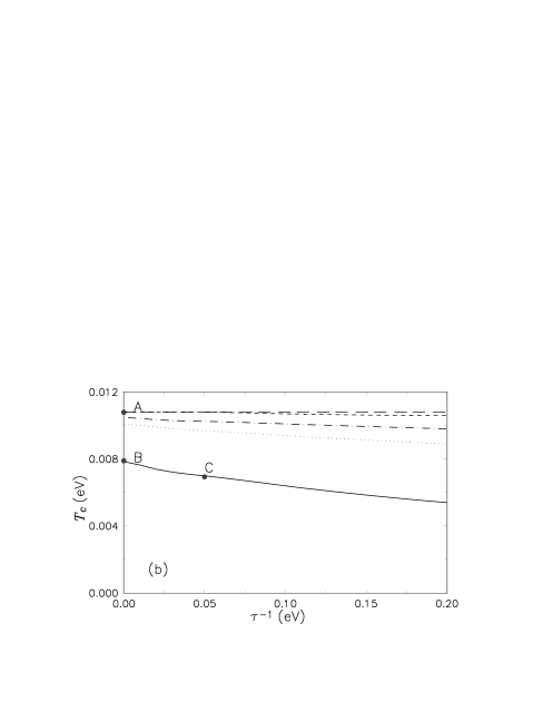
FIG. 1.: Transition temperature, $T_{c}$, as a function of impurity scattering rate, $\tau^{-1}$, for half-filled finite bandwidth superconductors, as calculated from Eq. 6. Fig. 1(a) is for $N_{F}\alpha^{2}$ = 0.02 eV and Fig. 1(b) for 0.05 eV. The solid, dotted, dot-dashed, short-dashed, and long-dashed curves represent, respectively, bandwidth $W$ = 0.1, 0.5, 1, 5, and 10 eV. The dots labeled as A, B, and C in Fig. 1(b) are selected for calculating NMR relaxation rates shown in Fig. 3. $T_{c}$ is decreased by impurity scatterings for finite bandwidth supercondcutors, while it is unchanged for those with infinite bandwidths. The rate of $T_{c}$ suppression by impurities is larger for narrower bandwidth superconductors.

The qualitative discussion above is well verified in the detailed numerical calculations. In Fig. 1, we show the transition temperature $T_{c}$, calculated from Eq. (10), as a function of impurity scattering rate $\tau^{-1}$ for several bandwidths. We took following Bickers et al. [22]

$$F(\Omega)=\left\{\begin{array}[]{ll}\frac{1}{R}\biggl{[}\frac{1}{(\Omega-\omega_{0})^{2}+\Gamma^{2}}-\frac{1}{\Gamma_{c}^{2}+\Gamma^{2}}\biggr{]}&\text{for}~{}|\Omega-\omega_{0}|\leq\Gamma_{c},\\ 0&\text{otherwise},\end{array}\right.$$ (31)

with $\omega_{0}$ = 0.05 eV, $\Gamma_{c}=3\Gamma$ = 0.015 eV. $R$ is a normalization constant to make $\int_{0}^{\infty}d\Omega~{}F(\Omega)=1$. Using 200 Matsubara frequencies, self-consistency is reached within a few tens of iterations at a given temperature, except for temperatures close to $T_{c}$. The solid, dotted, dot-dashed, short-dashed, and long-dashed curves correspond, respectively, to $W$ = 0.1, 0.5, 1, 5, and 10 eV. We considered half-filled cases for simplicity, so that the Fermi energy $\epsilon_{F}=W/2$. Fig. 1(a) and (b) are for $N_{F}\alpha^{2}$ = 0.02 and 0.05 eV, respectively. The long-dashed curves representing $W$ = 10 eV, are indistinguishable from infinite bandwidth curves. As we expected from the qualitative analysis above, the impurity suppression of the transition temperature is more pronounced for narrower bandwidths. As the bandwidth becomes wider, however, the rate of $T_{c}$ suppression by impurity scatterings is smaller until $\epsilon_{F}\approx 1$, beyond which we are almost in the infinite bandwidth limit where $T_{c}$ is independent of the impurity scattering rate in accordance with the Anderson’s theorem.

We wish to consider how other transport properties of finite bandwidth superconductors, NMR relaxation rate for example, are altered in the following section. If the reduction in $T_{c}$ is due to time reversal symmetry breaking, the NMR coherence peak below $T_{c}$ will be reduced. If, on the other hand, it is due to reduction of the effective electron-phonon coupling as is the case we consider here, we expect that the NMR coherence peak will be enhanced. This is because the strong-coupling effects cause phonon dampings and reduce the coherence peak as was discussed.

IV Nuclear Spin-Lattice Relaxation Rate

To calculate nuclear spin-lattice relaxation rate $T_{1}^{-1}$, we need to perform analytic continuation to obtain the gap and renormalization functions on real frequency, $\widetilde{\Delta}(\omega)$ and $\widetilde{Z}(\omega)$, from those on imaginary frequency, $\widetilde{\Delta}(ip_{n})$ and $\widetilde{Z}(ip_{n})$. It was carried out via the iterative method by Marsiglio, Schossmann, and Carbotte (MSC) [21]. The MSC equation which relates the gap and renormalization functions on imaginary frequency with those on real frequency, extended to half-filled finite bandwidth impure superconductors, is given by

$$\widetilde{Z}(\omega) = 1+\frac{i}{\omega}\int_{-\infty}^{\infty}d\Omega~{}\alpha^{2}F(\Omega)\frac{2\widetilde{\theta}(\omega-\Omega)~{}(\omega-\Omega)}{\sqrt{(\omega-\Omega)^{2}-\widetilde{\Delta}(\omega-\Omega)^{2}}}\Bigl{[}N(\Omega)+f(\Omega-\omega)\Bigr{]}$$ (32)

$$+ \frac{1}{\beta\omega}\sum_{n\geq 0}\frac{2\widetilde{\theta}_{n}ip_{n}}{\sqrt{p_{n}^{2}+\widetilde{\Delta}_{n}^{2}}}\Bigl{[}\lambda(\omega-ip_{n})-\lambda(\omega+ip_{n})\Bigr{]}+\frac{i}{\pi\tau\omega}\frac{\widetilde{\theta}(\omega)\omega}{\sqrt{\omega^{2}-\widetilde{\Delta}(\omega)^{2}}},$$ (33)

$$\widetilde{\Delta}(\omega) = \frac{i}{\widetilde{Z}(\omega)}\int_{-\infty}^{\infty}d\Omega~{}\alpha^{2}F(\Omega)\frac{2\widetilde{\theta}(\omega-\Omega)~{}\widetilde{\Delta}(\omega-\Omega)}{\sqrt{(\omega-\Omega)^{2}-\widetilde{\Delta}(\omega-\Omega)^{2}}}\Bigl{[}N(\Omega)+f(\Omega-\omega)\Bigr{]}$$ (34)

$$+ \frac{1}{\beta\widetilde{Z}(\omega)}\sum_{n\geq 0}\frac{2\widetilde{\theta}_{n}\widetilde{\Delta}_{n}}{\sqrt{p_{n}^{2}+\widetilde{\Delta}_{n}^{2}}}\Bigl{[}\lambda(\omega-ip_{n})+\lambda(\omega+ip_{n})\Bigr{]}+\frac{i}{\pi\tau\widetilde{Z}(\omega)}\frac{\widetilde{\theta}(\omega)\widetilde{\Delta}(\omega)}{\sqrt{\omega^{2}-\widetilde{\Delta}(\omega)^{2}}},$$ (35)

where

$$\lambda(\omega\pm ip_{n})=N_{F}\int_{0}^{\infty}d\Omega~{}\frac{2\Omega~{}\alpha^{2}F(\Omega)}{\Omega^{2}-(\omega\pm ip_{n})^{2}}.$$ (36)

This equation is solved iteratively for $\widetilde{Z}(\omega)$ and $\widetilde{\Delta}(\omega)$, taking $\widetilde{Z}_{n}$ and $\widetilde{\Delta}_{n}$, solution to the Eliashberg equation on Matsubara frequencies of Eq. (10), as an input, until self-consistency is reached. We show in Fig. 2 the gap function $\widetilde{\Delta}(\omega)$ as a function of $\omega$ at $T$ = 0.001 eV. We took the impurity scattering rate $\tau^{-1}$ = 0, and the phonon spectral function $\alpha^{2}F(\Omega)$ as given by Eq. (31) with $N_{F}\alpha^{2}=0.05$ eV which corresponds to Fig. 1(b). Fig. 2(a) is for an infinite bandwidth, and (b) is for bandwidth $W$ = 1 eV. The solid and dashed lines, respectively, stand for real and imaginary parts of the gap function. The obtained results for $W\rightarrow\infty$, where previous studies are available, are in good agreement with the published data [22].

FIG. 2.: The gap function, $\Delta(\omega)$, as a function of $\omega$ at $T$ = 0.001 eV. We took $\tau^{-1}$ = 0 and $N_{F}\alpha^{2}$ = 0.05 eV, which corresponds to Fig. 1(b). The solid and dashed lines, respectively, represent the real and imaginary parts of the gap. Fig. 2(a) is for an infinite bandwidth, and (b) is for $W$ = 1 eV.

The nuclear spin-lattice relaxation rate $T_{1}^{-1}$ is given by [23]

$$\frac{1}{T_{1}}=\lim_{\omega\rightarrow 0}\frac{1}{1-e^{-\beta\omega}}\sum_{\vec{q}}\Big{|}A_{q}\Big{|}^{2}Im\Bigl{[}\chi_{+-}(\omega+i\delta,\vec{q})\Bigr{]},$$ (37)

where $A_{q}$ is a form factor related with the conduction electron wavefunctions, and $\chi_{+-}(\omega,\vec{q})$ is a spin-spin correlation function at frequency $\omega$ and momentum transfer $\vec{q}$. The impurity scatterings are included in the self-energy of renormalized Green’s function. For a finite bandwidth, it is easy to derive

$$\frac{1}{T_{1}T} \propto \int_{0}^{\infty}d\epsilon\frac{\partial f(\epsilon)}{\partial\epsilon}~{}\biggl{\{}\biggl{[}Re\biggl{(}\frac{\epsilon~{}\widetilde{\theta}(\epsilon)}{\sqrt{\epsilon^{2}-\widetilde{\Delta}(\epsilon)^{2}}}\biggr{)}\biggr{]}^{2}+\biggl{[}Re\biggl{(}\frac{\widetilde{\Delta}(\epsilon)~{}\widetilde{\theta}(\epsilon)}{\sqrt{\epsilon^{2}-\widetilde{\Delta}(\epsilon)^{2}}}\biggr{)}\biggr{]}^{2}\biggr{\}}.$$ (38)

$$\rightarrow \int_{\Delta}^{\infty}d\epsilon\frac{\partial f}{\partial\epsilon}~{}\biggl{\{}\frac{\epsilon^{2}+\Delta^{2}}{\epsilon^{2}-\Delta^{2}}\biggr{\}},$$ (39)

where the $\widetilde{\Delta}(\epsilon)$ and $\widetilde{\theta}(\epsilon)$ are obtained by solving Eqs. (10) and (35) iteratively. The standard strong-coupling expression for $T_{1}^{-1}$ given, for example, by Fibich [24] can be obtained by putting $\widetilde{\theta}=\pi/2$ for infinite bandwidth. Eq. (39) follows for infinite bandwidth weak-coupling limit.

Before we present the detailed numerical calculations, let us first analyze the expression for $(T_{1}T)^{-1}$ of Eq. (38) qualitatively. For $T>T_{c}$, $\widetilde{\Delta}$ = 0 in Eq. (38), and

$$\widetilde{\theta}(\epsilon)=\tan^{-1}\biggl{[}\frac{iW}{2\epsilon\widetilde{Z}(\epsilon)}\biggr{]}=\left\{\begin{array}[]{ll}i\tanh^{-1}\biggl{[}\frac{W}{2\epsilon\widetilde{Z}(\epsilon)}\biggr{]}&{\rm for}~{}\epsilon\geq\frac{W}{2\widetilde{Z}},\\ \frac{\pi}{2}+i\tanh^{-1}\biggl{[}\frac{2\epsilon\widetilde{Z}(\epsilon)}{W}\biggr{]}&{\rm for}~{}\epsilon\leq\frac{W}{2\widetilde{Z}}.\end{array}\right.$$ (42)

Taking $\widetilde{Z}(\epsilon)\approx 1$ for simplicity, we have $Re\Bigl{[}\widetilde{\theta}(\epsilon)\Bigr{]}=\pi/2$ for $\epsilon\leq W/2$, and 0 for $\epsilon>W/2$. Then,

$$\frac{1}{T_{1}T}\propto\int_{0}^{W/2} d\epsilon \frac{\partial f(\epsilon)}{\partial\epsilon}=-\frac{1}{2}\tanh\Bigl{[}\textstyle{\frac{1}{2}}\beta W\Bigr{]},$$ (43)

$${\rm or,}~{}~{}\frac{(T_{1}T)_{n}}{(T_{1}T)_{s}} = \frac{\tanh\Bigl{[}W/2T\Bigr{]}}{\tanh\Bigl{[}W/2T_{c}\Bigr{]}}.$$ (44)

$(T_{1}T)_{n}/(T_{1}T)_{s}$, therefore, decreases as the temperature is increased, which is contrasted with the constant value of 1 for the infinite bandwidth case. The decrease of $(T_{1}T)_{n}/(T_{1}T)_{s}$ as the temperature is increased above $T_{c}$ was observed in the ⁵¹V NMR study of V₃Si superconductors by Kishimoto et al. [25]. This observation was interpreted in terms of narrow bandwidths in accord with the present work. The range of integration from 0 to $W/2$ is just what we may expect intuitively. The $T<T_{c}$ region, on the other hand, is difficult to analyze without detailed information on $\widetilde{\Delta}(\epsilon)$, because the height of NMR coherence peak is mainly determined by the magnitude of imaginary part of $\widetilde{\Delta}(\epsilon)$ in the Eliashberg formalism. We may expect, however, that the coherence peak will be enhanced as $W$ is decreased and $\tau^{-1}$ is increased, because $\lambda_{eff}$ is reduced.

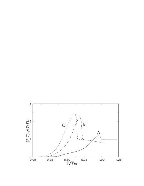
FIG. 3.: The normalized nuclear spin-lattice relaxation rate by the normal state Korringa value, $(T_{1}T)_{n}/(T_{1}T)_{s}$, as a function of the reduced temperature, $T/T_{c0}$, where $T_{c0}$ is the critical temperature of infinite bandwidth case, with $N_{F}\alpha^{2}$ = 0.05 eV. The solid, dot-dashed, and dashed curves, labeled, respectively, as A, B, and C, are computed for $W$ and $\tau^{-1}$ equal to 10 and 0, 0.1 and 0, and 0.1 and 0.05 eV, as can be read off from their counterparts in Fig. 1(b). The normalized relaxation rates show progressively enhanced peaks as one goes from A to B to C. This can be understood in terms of the effective electron-phonon coupling constant alone, because large $\lambda_{eff}$ suppresses NMR coherence peak due to strong-coupling phonon dampings. As $W$ is reduced and $\tau^{-1}$ is increased, $\lambda_{eff}$ is reduced. The computed $\lambda_{eff}$ for A, B, and C are 1.67, 0.63, and 0.60, respectively.

In Fig. 3, we show the normalized NMR relaxation rate by the normal state Korringa value, $(T_{1}T)_{n}/(T_{1}T)_{s}$, calculated from Eqs. (10), (35) and (38) as a function of $T/T_{c0}$, where $T_{c0}$ is the critical temperature for infinite bandwidth case. We took the phonon spectral function $\alpha^{2}F(\Omega)$ as given by Eq. (31) with $N_{F}\alpha^{2}=0.05$ eV, which corresponds to Fig. 1(b). We selected 3 sets of $W$ and $\tau^{-1}$ values, labeled as A, B, and C in Fig. 1(b), for $T_{1}^{-1}$ calculations. $W$ and $\tau^{-1}$ of A, B, and C are, respectively, in unit of eV, 10 and 0, 0.1 and 0, and 0.1 and 0.05, as can be read from Fig. 1(b). Note that as one goes from A to B to C, the normalized NMR relaxation rates have progressively enhanced peaks, and $T_{c}$ is reduced accordingly. These results are straightforward to interpret, as already explained before. The computed values of $\lambda_{eff}$ for A, B, and C are 1.67, 0.63, and 0.60, respectively. As $\lambda_{eff}$ is decreased, $T_{c}$ should be reduced and NMR coherence peak should be enhanced, because there is no time reversal symmetry breaking in the present problem. The solid curve of A, having $\lambda_{eff}$ = 1.67, has substantially reduced coherence peak, in agreement with the previous works [16, 17]. Note also that the normalized NMR relaxation rates for finite bandwidths decrease as $T$ is increased beyond $T_{c}$ as expected.

V Summary and Concluding Remarks

In this paper, we have investigated the effects of a finite bandwidth on the thermodynamic properties of impure superconductors within the framework of phonon-mediated Eliashberg theory. We found that the transition temperature and NMR coherence peak are suppressed and enhanced, respectively, by impurity scatterings when the finiteness of bandwidths is explicitly taken into consideration. These results can be understood in terms of reduced effective electron-phonon coupling $\lambda_{eff}$. The motivation for this work was, in part, the observation that the phonon frequency and the Fermi energy are comparable and a substantial disorder is present in the fullerene superconductors [4]. The NMR coherence peak in $(T_{1}T)^{-1}$ was found absent for doped fullerenes [26, 27]. We wish to point out that the present theory is $not$ concerned with why the NMR coherence peak is absent for a given material. The present theory shows that if the disorder is increased for a finite bandwidth superconductor, its transition temperature should be reduced and coherence peak should be enhanced, respectively, compared with those of a clean material. In view of our results, it will be very interesting to systematically investigate how the transition temperature and NMR coherence peak behave as the degree of disorder is varied for doped C₆₀.

In A₃C₆₀, almost all other experiments than NMR relaxation rates seem to point to a phonon-mediated $s$-wave pairing [4]. Also, due to the orientational disorder [28], the Fermi surface anisotropy is not strong enough to suppress the coherence peak [29]. The present study shows that a quite strong electron-phonon coupling of $\lambda_{eff}\approx 2$ is needed to suppress the NMR coherence peak in agreement with Nakamura $et~{}al.$ [16], and Allen and Rainer [17]. The $\lambda_{eff}\approx 2$ seems too large for doped fullerenes since the far infrared reflectivity measurements of DeGiorge et al. [30] show that $2\Delta/k_{B}T_{c}\approx 3.44-3.45$, a classic weak-coupling value. Because there are no magnetic impurities in A₃C₆₀, the absence of NMR coherence peak is still to be understood. Stenger et al. [31] suggested that the applied magnetic field is responsible for the suppressed NMR coherence peak. Their explanation, however, seems to be more a puzzle than an answer. According to the Eliashberg theory, the energy of applied magnetic field should be at least $\hbar\omega\approx 0.1\Delta$ to suppress the coherence peak. The magnetic field in their ¹³C NMR experiment corresponds to $\hbar\omega\approx 10^{-5}\Delta$. Such a small energy scale in the coherence peak suppression is really a puzzle. We are currently investigating the strong Coulomb interaction effects with a paramagnon approximation [19]. We suspect that the strong Coulomb interaction may be responsible for suppressed NMR coherence peak in doped fullerenes.

This work was supported by Korea Science and Engineering Foundation (KOSEF) through Grant No. 951-0209-035-2, and by the Ministry of Education through Grant No. BSRI-95-2428.

REFERENCES

[1] J. R. Schrieffer, Theory of Superconductivity,
Addison-Wesley (1964).
[2] P. B. Allen and B. Mitrovic, in Solid State Physics
Vol. 37, edited by F. Seitz et al., Academic Press (1982), p. 1, and
references therein.
[3] W. E. Pickett, Phys. Rev. B 26, 1186 (1982).
[4] A. F. Hebard, Physics Today 45 No. 11, 26 (1992), and
references therein.
[5] J. Bardeen, L. N. Cooper, and J. R. Schrieffer, Phys. Rev.
108, 1175 (1957).
[6] H. Zheng and K. H. Bennemann, Phys. Rev. B 46,
11993 (1992).
[7] F. Marsiglio, Phys. Rev. B 45, 956 (1992).
[8] A. A. Abrikosov, L. P. Gorkov, and I. E. Dzyloshinski,
Methods of Quantum Field Theory in Statistical Physics, Dover (1965),
chap. 7.
[9] K. Maki, in Superconductivity,
edited by R. D. Parks, Dekker (1967), p. 1035.
[10] Y. J. Kim and A. W. Overhauser, Phys. Rev. B 47,
8025 (1993); ibid.49, 12339 (1994);
A. A. Abrikosov and L. P. Gorkov, ibid.49,
12337 (1994).
[11] P. W. Anderson, J. Phys. Chem. Solid 11, 26 (1959).
[12] R. J. Radtke, preprint cond-mat/9306037, and
Ph.D. thesis, University of Chicago, Appendix C, (1994).
[13] D. Fay and J. Appel, Phys. Rev. B 51, 15604 (1995).
[14] D. E. McLaughlin, in Solid State Physics
Vol. 31, edited by H. Ehrenreich et al., Academic Press (1976), p. 1,
and references therein.
[15] H. Y. Choi and E. J. Mele, Phys. Rev. B 52, 7549
(1995).
[16] Y. O. Nakamura et al., Solid State Commun.
86, 627 (1993).
[17] P. B. Allen and D. Rainer, Nature 349, 396 (1991).
[18] T. Koyama and M. Tachiki, Phys. Rev. B 39,
2279 (1989).
[19] H. Hasegawa, J. Phys. Soc. Jpn. 42, 779 (1977).
[20] A. H. MacDonald, Phys. Rev. B 24, 1130 (1981).
[21] F. Marsiglio, M. Schossmann, and J. P. Carbotte, Phys. Rev. B
37, 4965 (1988).
[22] N. E. Bickers et al., Phys. Rev. B 42,
67 (1990).
[23] T. Moriya, J. Phys. Soc. Jpn. 18, 516 (1963).
[24] M. Fibich, Phys. Rev. Lett. 14, 561 (1965);
ibid., 621 (1965).
[25] Y. Kishmoto, T. Ohno, and T. Tanashiro,
J. Phys. Soc. Jpn. 64, 1275 (1995).
[26] R. Tycko et al., Phys. Rev. Lett. 68,
1912 (1992).
[27] S. Sasaki, A. Matsuda, and C. W. Chu, J. Phys. Soc. Jpn.
63, 1670 (1994).
[28] P. W. Stephens et al., Nature 351,
632 (1991).
[29] E. J. Mele, unpublished.
[30] L. DeGiorge et al., Nature 369, 541 (1994).
[31] V. A. Stenger, C. H. Pennington, D. R. Buffinger,
and R. P. Ziebarth, Phys. Rev. Lett 74, 1649 (1995).