Contacts and Edge State Equilibration in the Fractional Quantum Hall Effect

Abstract

We develop a simple kinetic equation description of edge state dynamics in the fractional quantum Hall effect (FQHE), which allows us to examine in detail equilibration processes between multiple edge modes. As in the integer quantum Hall effect (IQHE), inter-mode equilibration is a prerequisite for quantization of the Hall conductance. Two sources for such equilibration are considered: Edge impurity scattering and equilibration by the electrical contacts. Several specific models for electrical contacts are introduced and analyzed. For FQHE states in which edge channels move in both directions, such as $\nu=2/3$, these models for the electrical contacts do not equilibrate the edge modes, resulting in a non-quantized Hall conductance, even in a four-terminal measurement. Inclusion of edge-impurity scattering, which directly transfers charge between channels, is shown to restore the four-terminal quantized conductance. For specific filling factors, notably $\nu=4/5$ and $\nu=4/3$, the equilibration length due to impurity scattering diverges in the zero temperature limit, which should lead to a breakdown of quantization for small samples at low temperatures. Experimental implications are discussed.

]

I Introduction

An important lesson learned from studies of mesoscopic structures is that the transport properties of a system can be strongly influenced by the electrical contacts used to make the measurements[1]. The nature of the contacts can be particularly important in the quantum Hall regime, where transport takes place via edge states. Current carrying contacts feeding the edge states can alter their population, leaving the edge out of equilibrium. High impedance voltage contacts selectively measure the electrochemical potential of the edge modes to which they are most strongly coupled.

In the integer quantum Hall effect, Büttiker[2] has generalized Landauer quantum transport theory[3] to incorporate the effects of multiple electrical contacts. A contact, or lead, is modeled as a large reservoir in equilibrium at an electro-chemical potential $\mu$. The edge states in the sample are populated by electrons incident from the leads. Büttiker defines an “ideal” contact as one in which no scattering occurs at the contact. The edge states emanating from such ideal contacts are thus populated in equilibrium at the chemical potential $\mu$. Büttiker also discusses the more generic case of a disordered or “non ideal” contact, which is characterized by transmission and reflection matrices between the edge channels in the “sample” and in the “leads”.

At integer filling factors $\nu>1$, there are multiple edge channels. For generic “non-ideal” contacts, the coupling to the different edge modes will be different. Non-ideal current contacts will thus tend to populate the edge modes differently, putting them out of equilibrium with one another. In this case, the edge is not characterized by a unique chemical potential, and the Hall conductance measured using similar non-ideal voltage contacts will not be quantized. For this reason, Büttiker emphasizes the important role played by inter-channel electron scattering, which can re-equilibrate the different modes. Provided the separation between current and voltage leads is greater than the equilibration length, the voltage lead will measure an equilibrated edge, giving a quantized Hall conductance.

By fabricating non-ideal contacts which are close together, it is possible to study directly the equilibration between edge states. Indeed, in beautiful experiments utilizing a quantum point contact which selectively populates channels[4, 5, 6], equilibration lengths of order $40\mu m$ have been measured in the integer quantum Hall regime.

While the importance of contacts and edge state equilibration is well appreciated for the integer quantum Hall effect, a suitable generalization to the fractional quantum Hall regime has been lacking. In the fractional quantum Hall effect (FQHE), the edge modes cannot be described in terms of a free electron model, so that a Landauer-Büttiker description of edge transport is not possible. Recently a powerful framework for describing edge states in the FQHE has been developed, based on the chiral Luttinger liquid model[7]. This description enables one to compute transport properties of edge states in the FQHE. Recently, the effects of impurity scattering on edge state equilibration has been discussed in the FQHE[8, 9], but the role of electrical contacts has not been adequately addressed[10].

In this paper we develop a simple theory for edge state transport in the FQHE which allows for incorporation of electrical contacts and inter-mode equilibration. The approach is based on a simple kinetic equation for the edge state dynamics, which closely resembles a linearized Boltzmann equation. Coupling to electrical contacts is incorporated by adding source terms to the kinetic equation, loosely analogous to scattering terms in the Boltzmann equation. Impurity scattering between multiple edge modes can also be simply incorporated into the kinetic equation. Several specific models for the contacts are considered, which are analogous to Büttiker’s “ideal” and “non ideal” contacts in the IQHE.

For simplicity we focus on quantum Hall states at filling $\nu=(p_{1}-1/p_{2})^{-1}$ ($p_{1}$ odd, $p_{2}$ even), which correspond to the second level of the Haldane-Halperin hierarchy[11] and have two edge channels. As in the integer quantum Hall effect, we find that equilibration between the different edge channels is a prerequisite for the quantization of the Hall conductance. There are two sources for this equilibration which we address separately: Impurity scattering along the edge and equilibration by the contacts themselves. In the former case, we find important differences with the IQHE. Specifically, for filling fractions with $|p_{2}|=4,6,...$, such as $\nu=4/3,4/5,...$, the inter-mode equilibration length due to impurity scattering is temperature dependent and diverges at low temperatures. In this case, for finite sized sample, quantization of the Hall conductance should break down at very low temperatures.

There are also important differences between the integer and fractional Hall effects with regards the equilibration taking place at the contacts. The differences are most pronounced when the two fractional edge modes are moving in opposite directions, for $p_{2}<0$ at filling $\nu=2/3,4/5,...$. In this case, even ”ideal contacts” are insufficient to equilibrate the two edge modes. The reason is that the two modes emanate from different reservoirs, at different chemical potentials. Then in the absence of any direct inter-mode impurity tunneling, the two channels on the same edge will be at different chemical potentials. Impurity scattering away from the contacts can still cause equilibration, but with an equilibration length diverging at low temperatures for $|p_{2}|\geq 4$. In contrast, when both edge modes propagate in the same direction ($p_{2}>0$), we show that “ideal contacts” can be defined which completely equilibrate the two channels, just as in the IQHE.

In this paper we focus almost exclusively on the linear response conductances, for a sample with finite width, $L$. Within linear response, both the Hall voltage drop $V_{H}$, and the Hall electric field $E=V_{H}/L$, are taken to zero, with fixed width $L$. In this limit, the edge currents give an order one contribution to the Hall conductance, and with long-ranged forces screened by a ground plane, dominate completely over bulk contributions. As we shall see, the conductance in this case is a “mesoscopic” quantity, which can depend on the nature of the electrical contacts and of the edge states which transport current between them. In contrast, it is possible to define a “macroscopic” Hall conductance which is a bulk property, independent of the edge dynamics. In the limit that $L\rightarrow\infty$, with fixed finite electric field, $E$, the edge contribution to the bulk Hall conductance vanishes as $1/L$.

Our paper is organized as follows. In section II, we introduce the simple kinetic equation description of FQHE edge state transport, for the case in which only a single edge mode is expected, $\nu^{-1}$ an odd integer. Various models for electrical contacts are discussed within this framework. In section III, the description is generalized to describe hierarchical Hall states with two edge modes. Equilibration between the two edge modes both at the contacts, and due to edge impurity scattering, is discussed. In section IV, we describe several specific experimental consequences, and conclude in Section V.

II SINGLE EDGE MODE

In this section we introduce a simple kinetic equation description for the edge of a Laughlin state at filling $\nu=1/m$. In this case there is only a single edge mode, which satisfies a simple continuity equation. We then show how electrical contacts can be incorporated into this approach, and consider specific models for the contacts. Finally, we show how bulk electric fields, and bulk currents, can also be incorporated, without changing the conclusions. In Section III we will turn our attention to hierarchical Hall states, which have multiple edge modes.

A Kinetic Equation

For filling $\nu=1/m$ with odd integer $m$, a single chiral edge mode is expected[7]. The 1d electron density, $n(x)$, satisfies a simple equation of motion,

$$\partial_{t}n+v\partial_{x}n=0,$$ (1)

which describes waves moving in one direction at velocity $v$: $n(x,t)=f(x-vt)$, for arbitrary $f$. This can be written as a continuity equation,

$$\partial_{t}n+\partial_{x}J=0,$$ (2)

with an edge current defined as

$$J=vn.$$ (3)

Eqn. (2.2) is a conservation law for electric charge at the edge. Together, (2.2) and (2.3) are a simple kinetic equation for edge charge transport.

Since the bulk is incompressible, charge cannot pass from the edge into the bulk, at least in linear response. In the presence of a large non-linear driving field, though, bulk currents can flow, and it is necessary to augment eqn. (2.2). Moreover, charge can be added or removed from the edge mode at contacts. In these cases source terms must be added to the right side of (2.2):

$$\partial_{t}n+\partial_{x}J=I_{bulk}(x)+I_{c}(x),$$ (4)

which describe charge being added or removed from the edge, via either bulk currents, or from contacts.

The kinetic equation (2.4) is analogous to the transport equation for quasiparticles in a Fermi liquid[12]. In the present case, the Fermi surface is replaced by a single point. The left hand side describes collisionless transport, and follows directly from microscopic equations of motion, as we show below. The term on the right hand side coming from the contacts is analogous to a “collision term” in the Boltzmann equation. An explicit form for this term can be obtained by using Fermi’s Golden rule, as we show below, which is the rough equivalent of the relaxation time approximation. This treatment requires that the time between successive tunneling events from the contacts exceeds the dephasing time $\tau_{\phi}$. We shall describe the role of the bulk currents in section 2C.

We now show briefly that the collisionless terms (2.2) and (2.3) follow directly from a chiral Luttinger liquid[7] description of the edge mode. In terms of a boson field, $\phi$, related to the electron density via $n(x)=(1/2\pi)\partial_{x}\phi$, the chiral Luttinger Hamiltonian is simply:

$$H={v\over{4\pi\nu}}\int dx(\partial_{x}\phi)^{2},$$ (5)

where the phase field satisfies a Kac-Moody commutation relation:

$$[\phi(x),\phi(x^{\prime})]=i\pi\nu{\rm sgn}(x-x^{\prime}).$$ (6)

¿From the Heisenberg equations of motion for the operator $\phi$, it is straightforward to show that the density operator satisfies the kinetic equation (2.1).

The continuity equation (2.2) can be re-written in the suggestive form: $\partial_{x}(J+(\partial_{t}\phi/2\pi))=0$, allowing us to identify the current operator as $J=-\partial_{t}\phi/2\pi$. It is useful to assume normal ordering, so that in equilibrium both the density and currents vanish. In the presence of a non-zero chemical potential, $\mu$, however, currents will flow. The current response can be deduced by adding to the Hamiltonian a term of the form:

$$\delta H=-\mu\int dxn,$$ (7)

and then evaluating the current, $J=-e\partial_{t}\phi/2\pi$, using the commutation relations (2.6). One deduces a non-vanishing transport current of the form:

$$J=\nu{e\over h}\mu.$$ (8)

The conductance is seen to be appropriately quantized, $G=eJ/\mu=\nu e^{2}/h$.

B Contacts

We consider now incorporating electrical contacts into the above description of edge transport. We begin by discussing Büttiker’s “ideal” contact[2] model generalized to the fractional quantum Hall regime. While this model is useful for performing simple calculations, it is rather unrealistic - particularly in the FQHE - since it assumes that the edge modes retain their integrity deep within the reservoirs. As an alternative, we consider a contact modeled as a tunnel junction to a metallic electrode. In Büttiker’s terminology, this is an example of a “non ideal” contact. The point contact tunnel junction can be suitably generalized, however, into a tunnel junction “line contact”. The “line contact” is shown to be “ideal”, with vanishing contact resistance.

1 The Ideal Contact

In the Landauer-Büttiker approach to quantum transport, electrical contacts are modeled as reservoirs at chemical potential $\mu$. Transport is viewed as a scattering process. Electrons incident from the reservoirs enter the sample, scatter about and then leave the sample back into the reservoirs. In this scheme an “ideal contact” is one in which there is no electron backscattering during the process of entering or leaving the sample. The population of an each edge mode is then determined by the chemical potential of the reservoir from which it emanates.

For an interacting system, such as a FQHE edge mode, the transport can not be described in terms of the population of free electron states. Nonetheless, a Landauer-type formula for transport can be derived within a linear response Kubo formulation [13, 14]. The “reservoir” is modeled as a semi-infinite strip of FQHE fluid connected to the “sample”. The edge channels extend to infinity in the “reservoirs”, as shown in Fig. 1a. Following Fisher and Lee, the conductance may then be computed within linear response theory by applying a time dependent potential, $V(x)e^{i\omega t}$, where $V(x)$ is equal to $\mu_{i}$ in the i’th reservoir, and then taking the $\omega\rightarrow 0$ limit. For non interacting electrons this procedure is equivalent to the Landauer approach, but can be suitably generalized to the FQHE. It results in a non-equilibrium current flowing in the fractional edge channels, determined by the chemical potential of the reservoir from which they emanate, $J=\nu(e/h)\mu_{i}$. If the Hall voltage is measured on the top and bottom edges by similar “ideal contacts”, the result is an appropriately quantized Hall conductance. Moreover, the two terminal conductance, defined as the ratio of the current to the source-drain voltage, is also quantized.

The assumption that the edge modes maintain their integrity deep within the reservoirs is highly unphysical. This feature is particularly worrisome in the FQHE, where the the edge modes are gases of fractionally charged quasiparticles. One would expect an appreciable contact resistance as the electrons from the metallic electrodes splinter upon entering the sample, in contrast to the resistanceless “ideal contacts” considered above. We now consider more realistic models for electrical contacts, consisting of a metallic electrode coupled to the edge modes via tunnel junctions.

2 The tunnel junction point contact

Consider a metallic electrode, described by a Fermi liquid at chemical potential $\mu$. The electrode is connected to the edge mode via a tunnel junction, at position $x=0$. The tunneling process transfers an electron from metallic electrode to the edge with Hamiltonian:

$$H_{tun}=-t_{0}\psi(x=0)\int dx\delta(x)e^{i\phi(x)/\nu}+h.c..$$ (9)

Here $\psi$ is an electron destruction operator in the metallic electrode, and $e^{i\nu\phi}$ is the edge electron creation operator. This tunneling Hamiltonian leads to an additional term on the right side of the continuity equation (2.2),

$$\hat{I}_{c}=\delta(x)it_{0}\psi(x)e^{i\phi(x)/\nu}-h.c.,$$ (10)

which describes tunneling of charge from electrode to edge. Since this operator is non-linear, it is desirable to replace it by it’s expectation value, so that (2.2) can still be used as a classical kinetic equation. This simplification requires that successive tunneling events are incoherent. In the limit $t_{0}\rightarrow 0$ this should be the case, since the time between tunneling events then exceeds the electron dephasing times both in the electrode and on the edge. In this limit, the average tunneling current is given by a contact conductance, $G_{c}$, times the chemical potential drop between electrode and the edge mode. The chemical potential of the edge mode can be obtained from the upstream current entering the contact region: $\mu_{edge}=J(x=0^{-})h/(\nu e)$. Thus the kinetic equation can written as a closed expression in terms of the edge density and current:

$$\partial_{t}n+\partial_{x}J=I_{c}(x),$$ (11)

with a contact current:

$$I_{c}(x)=\delta(x)G_{c}\left(\mu-{h\over{\nu e}}J(x)\right).$$ (12)

When many contacts are present, at positions $x_{i}$, and chemical potentials $\mu_{i}$, this generalizes to

$$I_{c}(x)=\sum_{i}\delta(x_{i})G_{c}\left(\mu_{i}-{h\over{\nu e}}J(x_{i})\right).$$ (13)

The tunneling conductance will in general be temperature dependent. Using Fermi’s Golden rule perturbative in the tunneling matrix element $t_{0}$, gives $G_{c}\sim t_{0}^{2}T^{(1/\nu-1)}$, which vanishes at low temperature in the FQHE. We will assume in any event, that $G_{c}<<e/h$.

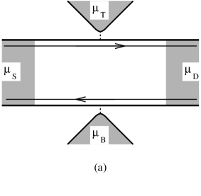
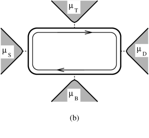
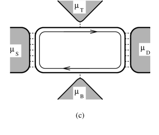
FIG. 1.: Three different models for the source and drain contacts to a quantum Hall fluid. (a) “ideal” contacts: the FQHE edge channels extend to infinity in both the source and drain electrodes; (b) tunnel junction point contacts; (c) tunnel junction line contacts. In (a), (b) and (c), the Hall voltage is measured via weakly coupled point contact tunnel junctions.

The large resistance associated with the contacts will dominate the resistance in a two-terminal measurement. To see this explicitly from the kinetic equation, consider a two-terminal geometry (Fig. 1b), with source electrode at $\mu_{S}$ and drain at $\mu_{D}$. In steady state, the time derivative can be dropped, and the kinetic equation can be readily solved. Denoting the current flowing along the top and bottom edges by $J_{T/B}$, one obtains from the kinetic equation,

$$J_{T}-J_{B}=G_{c}\left(\mu_{S}-{h\over{\nu e}}J_{B}\right),$$ (14)

$$J_{B}-J_{T}=G_{c}\left(\mu_{D}-{h\over{\nu e}}J_{T}\right),$$ (15)

where for simplicity we have assumed equal contact resistances, $G_{c}^{-1}$, for the source and drain electrodes. The transport current, $I=J_{T}-J_{B}$ is then found to be:

$$I\simeq{1\over 2}G_{c}(\mu_{S}-\mu_{D}),$$ (16)

under the assumption, $G_{c}<<h/e$. As expected, the two-terminal resistance is simply a sum of the two contact resistances, and is not quantized.

In a four terminal Hall measurement there are two additional voltage contacts, on the top and bottom edges, as shown in Fig. 1b. The chemical potentials in these contacts, denoted $\mu_{T/B}$, are set by the requirement that no net current flows from these electrodes into the sample. ¿From (2.12) this implies $\mu_{T}=J_{T}h/(\nu e)$ and $\mu_{B}=J_{B}h/(\nu e)$. The transport current, $I=J_{T}-J_{B}$, is then,

$$I={\nu e\over h}(\mu_{T}-\mu_{B}),$$ (17)

giving an appropriately quantized four-terminal Hall conductance.

As expected, we find a quantized four-terminal Hall conductance, independent of the contact resistance. As we show in Section III, this result breaks down when multiple edge modes are present - the four-terminal conductance is not quantized when measured with such non-ideal contacts.

3 The Tunnel Junction Line Contact

The above tunnel junction point contact model provides an explicit realization of a “non-ideal” contact, with large contact resistance. We now generalize this model to describe an “ideal contact” with vanishing contact resistance. Consider a metallic electrode which is coupled to the edge mode via tunneling, along a segment of length $L$. We refer to this as a “line junction” contact. The validity of a kinetic equation description again requires that successive tunneling events from electrode to edge are incoherent. This will be satisfied provided the tunneling conductance per unit length is sufficiently small. Since the contact length, $L$, can be made large, however, the total conductance between electrode and edge need not be small.

The kinetic equation is again given by (2.11). However, the tunneling current from the electrode is now extended over a length $L$,

$$I_{c}(x)=\sigma_{c}\left(\mu-{h\over{\nu e}}J(x)\right)\ \ \ \ {\rm for}\ \ \ \ 0<x<L$$ (18)

where $\sigma_{c}$ is the tunneling conductance per unit length. As before, $\sigma_{c}$ may be temperature dependent.

In a steady state, the kinetic equation simplifies to $\partial_{x}J(x)=I_{c}(x)$, and can be readily solved. In the region $0<x<L$, the solution for $J(x)$ is

$$J(x)={\nu e\over h}\mu+\left(J(x=0)-{\nu e\over h}\mu\right)e^{-x/\ell_{c}}$$ (19)

with an equilibration length defined by: $\ell_{c}=\nu\sigma_{c}^{-1}$. Provided $\ell_{c}<<L$, the edge mode equilibrates fully with the metallic electrode and $J(x>L)=\nu\mu$. The two-terminal conductance measured with “line contacts” is determined by considering currents on the top and bottom edges. Referring to Fig. 1c, we have $J_{T}=(\nu e/h)\mu_{S}$ and $J_{B}=(\nu e/h)\mu_{D}$, which gives for the transport current $I=J_{T}-J_{B}$:

$$I={\nu e\over h}(\mu_{S}-\mu_{D}).$$ (20)

The two-terminal conductance is quantized, indicating that the “contact resistance” vanishes. The “line contact” thus provides an explicit realization of an “ideal contact” for FQHE states with a single edge mode. Before discussing multiple edge modes, we briefly consider the role of bulk currents for $\nu^{-1}$ an odd integer.

C Bulk currents

A confusing aspect of transport in the quantum Hall effect is the relative importance of edge versus bulk currents. If the long-ranged Coulomb interactions are screened by a ground plane, one expects the linear response transport current to be confined to the edges. However, when Coulomb forces are unscreened, or one is well outside the linear response regime, additional bulk currents are expected, along with bulk electric fields. The total transport current will be a sum of the edge and bulk contributions. Likewise, the measured Hall voltage will be a sum of the edge chemical potentials and the bulk electric potential drop.

The distinction between edge and bulk currents becomes clear in the IQHE for non-interacting electrons. Consider the schematic plot of energy levels[15] in the lowest two Landau levels, as one transverses the sample, see Fig. 2. In 2(a) there is no bulk electric field - the Landau levels are flat and no bulk currents flow. In 2(b), the presence of a bulk electric field gives rise to a finite velocity $v=dE/dk$ of the bulk states, and hence a bulk current. In both cases, however, the total current, summing over both bulk and edge states, is given by $I=(e/h)(\mu_{T}-\mu_{B})$.

FIG. 2.: Dispersion of energy levels for non interacting electrons in a quantum Hall bar as a function of the one dimensional momentum $k$, which is related to the transverse position $y$. In (a) there is no electric field, so the bulk states in each Landau level are degenerate. In (b), there is a finite electric field in the bulk, which gives rise to a finite velocity $v=\partial E/\partial k$ for states in the bulk. In both cases the net current is determined by the electrochemical potentials at the two edges, $\mu_{T}$ and $\mu_{B}$.

This picture can readily be generalized to the FQHE. The total transport current in the x-direction is expressed as a sum of bulk and edge contributions

$$I=J_{T}-J_{B}+\int_{y_{B}}^{y_{T}}dy\ \ J^{x}_{\rm bulk},$$ (21)

where the bulk current density, defined between $y=y_{B}$ and $y=y_{T}$ near the top and bottom edges, is

$$\vec{J}_{\rm bulk}=\sigma_{xy}\hat{z}\times\vec{E}.$$ (22)

The edge currents on the top and bottom are denoted $J_{T}$ and $J_{B}$. The dividing lines, at $y_{T}$ and $y_{B}$, between the edge and bulk are arbitrary, so that $J_{T/B}$ is only defined up to an additive constant. This constant may be chosen so that the edge currents vanish in equilibrium. This is equivalent to normal ordering the edge current operator with respect to the equilibrium ground state.

In the presence of bulk electric fields, $\vec{E}$, the edge current is no longer conserved, since currents can flow from the edge into the bulk. The kinetic equation obeyed by the edge currents must therefore be modified,

$$\partial_{t}n_{T/B}+\partial_{x}J_{T/B}=\sigma_{xy}E_{x}(x,y_{T/B}),$$ (23)

for top and bottom respectively.

However, it is now a simple matter to eliminate the dependence on electric fields in the above two equations. In terms of an electric potential, $\vec{E}=\vec{\nabla}V$, we define new currents:

$$\tilde{J}_{T/B}=J_{T/B}-\sigma_{xy}V(x,y_{T/B}).$$ (24)

These new currents are conserved even with bulk electric fields present, since (2.23) can be re-written: $\partial_{t}n_{T/B}+\partial_{x}\tilde{J}_{T/B}=0$. Moreover, the total transport current becomes simply

$$I=\tilde{J}_{T}-\tilde{J}_{B}.$$ (25)

Notice that the new currents, $\tilde{J}_{T/B}$, satisfy the same steady-state kinetic equations as the edge currents do in the absence of bulk electric fields. Thus, the results of this and the next sections are not modified by the presence of bulk electric fields.

III MULTIPLE EDGE MODES

A Kinetic Equation

For hierarchical Hall states[11] there are multiple modes on a given edge. The structure of the edge modes is set by the topological order in the bulk, which is characterized by a square symmetric matrix $K$ [16, 17], with integer matrix elements. At the n’th level of the hierarchy the matrix $K$ is an n by n matrix. In addition there is a vector of integer “charges”, $t_{i}$. The filling factor is given by

$$\nu=\sum_{ij}t_{i}K^{-1}_{ij}t_{j}.$$ (26)

The explicit form of the $K$ matrix for a given quantum Hall state depends on the choice of basis, as do the integers $t_{i}$[16, 17]. For convenience we adopt throughout the “symmetric basis” in which $t_{i}=1$ for all $i$.

The form of the $K$-matrix determines the structure of edge excitations. In terms of $n$ bosonic fields, $\phi_{i}$, which satisfy commutation relations:

$$[\phi_{i}(x),\phi_{j}(x^{\prime})]=i\pi K^{-1}_{ij}{\rm sgn}(x-x^{\prime}).$$ (27)

the appropriate edge Hamiltonian is

$$H=\int dx{1\over{4\pi}}\sum_{ij}V_{ij}\partial_{x}\phi_{i}\partial_{x}\phi_{j}.$$ (28)

The matrix $V_{ij}$ is a non-universal positive definite matrix, depending on the edge confining potential and edge electron interactions. The Hamiltonian describes $n$ propagating chiral modes. The directions of propagation are determined by the signs of the eigenvalues of the $K$ matrix.

The total electronic charge density at the edge is given by

$$n_{\rho}(x)=\sum_{i}n_{i}(x)$$ (29)

where the density in the i’th mode is, $n_{i}=\partial_{x}\phi_{i}/2\pi$.

A kinetic equation description of edge transport follows again from the Heisenburg equations of motion, which can be cast in the form:

$$\partial_{t}n_{i}+\partial_{x}J_{i}=0,$$ (30)

with currents:

$$J_{i}=K^{-1}_{il}V_{lj}n_{j}.$$ (31)

The expression (3.6) relating currents and densities is analogous to the relationship between the current and density of quasiparticles in a Fermi liquid. The interaction terms $V_{ij}$ play a role very similar to that of the Fermi liquid parameters.

Once again, it is useful to assume normal ordering for the densities, $n_{i}$, so that in equilibrium all densities and currents vanish. With non-vanishing chemical potentials, $\mu_{i}$, however, currents will flow. As before, the currents can be computed by adding to the Hamiltonian:

$$\delta H=-\sum_{i}\int dx\mu_{i}n_{i},$$ (32)

and then evaluating the currents, $J_{i}=-e\partial_{t}\phi_{i}/2\pi$, using the commutation relations (3.2). This gives a non-vanishing transport current,

$$J_{i}=(e/h)K^{-1}_{ij}\mu_{j}.$$ (33)

When the edge modes are in equilibrium at a common chemical potential, $\mu_{i}=\mu$, the total edge current is appropriately quantized, as follows from (3.1):

$$J_{\rho}=\sum_{i}J_{i}={\nu e\over h}\mu.$$ (34)

However, if the edge modes are fed by non-ideal contacts, they will generally not all be at the same chemical potential. In this case, perfect Hall quantization can break down, as we detail below.

For simplicity we will focus hereafter on the special case of two edge modes, where $K$ is a 2 by 2 matrix. This includes bulk states at filling $\nu=1/(p_{1}-1/p_{2})$, with $p_{1}$ and $p_{2}$ odd and even integers, respectively. The explicit form for $K$ in the “symmetric” basis is:

$$K=\left(\begin{array}[]{cc}p_{1}&p_{1}-1\\ p_{1}-1&p_{1}+p_{2}-2\end{array}\right).$$ (35)

When $p_{1}=1$ the $K$ matrix is diagonal, with eigenvalues $1$ and $p_{2}-1$. When $p_{2}$ is positive, as for $\nu=4/3$ and $\nu=2$, both modes propagate in the same direction. For negative $p_{2}$, however, the two modes are predicted to propagate in opposite directions. This includes fillings $\nu=2/3$ and $\nu=4/5$.

As we shall see below, quantization of the Hall conductance when multiple modes are present, generally requires that the different modes on a given edge are equilibrated at a common chemical potential. For this reason it will be convenient to transform to a new set of fields which reveal more readily when an edge is equilibrated. To this end we define charge and neutral fields[8] via

$$\phi_{\rho} =\phi_{1}+\phi_{2},$$ (36)

$$\phi_{\sigma} =\phi_{1}+(1-p_{2})\phi_{2}.$$ (37)

The charge and neutral fields commute with one another, and satisfy:

$$[\phi_{\rho}(x),\phi_{\rho}(x^{\prime})]=i\pi\nu{\rm sgn}(x-x^{\prime}),$$ (38)

$$[\phi_{\sigma}(x),\phi_{\sigma}(x^{\prime})]=i\pi p_{2}{\rm sgn}(x-x^{\prime}).$$ (39)

Note that $p_{2}$ can be negative. The Hamiltonian becomes, $H=H_{\rho}+H_{\sigma}+H_{\rm int}$, with charge and neutral pieces

$$H_{\rho}={v_{\rho}\over{4\pi\nu}}\int dx(\partial_{x}\phi_{\rho})^{2}$$ (40)

$$H_{\sigma}={v_{\sigma}\over{4\pi|p_{2}|}}\int dx(\partial_{x}\phi_{\sigma})^{2}$$ (41)

coupled together via

$$H_{\rm int}={2v_{\rm int}\over{4\pi}}\int dx\partial_{x}\phi_{\rho}\partial_{x}\phi_{\sigma}.$$ (42)

The velocities $v_{\rho}$, $v_{\sigma}$ and $v_{\rm int}$ depend on the original velocities, $V_{ij}$ in (3.3).

The equations of motion for the charge and neutral fields can be obtained and expressed in terms of charge and neutral densities:

$$n_{\alpha}={1\over 2\pi}\partial_{x}\phi_{\alpha}$$ (43)

with $\alpha=\rho,\sigma$. Again, they can be written as continuity equations,

$$\partial_{t}n_{\alpha}+\partial_{x}J_{\alpha}=0$$ (44)

with currents defined as

$$J_{\rho}=v_{\rho}n_{\rho}+\nu v_{int}n_{\sigma},$$ (45)

and

$$J_{\sigma}={\rm sgn}(p_{2})v_{\sigma}n_{\sigma}+p_{2}v_{int}n_{\rho}.$$ (46)

Notice that for $p_{2}<0$, the neutral mode propogates in the direction opposite to the charge mode.

The charge and neutral currents can be given a simple physical interpretation. Using (3.11) the charge current can be expressed in terms of the original currents, $J_{i}$, as

$$J_{\rho}=J_{1}+J_{2}.$$ (47)

Thus $J_{\rho}$ is simply the total electrical charge current along the edge. Likewise, the neutral current takes the form

$$J_{\sigma}=J_{1}+(1-p_{2})J_{2}.$$ (48)

In the presence of non-vanishing chemical potentials, $\mu_{i}$, this can be re-expressed using (3.8) as:

$$J_{\sigma}={e\over h}(\mu_{1}-\mu_{2}).$$ (49)

When the edge is equilibrated, $\mu_{1}=\mu_{2}$, the neutral current vanishes, whereas a non-zero $J_{\sigma}$ indicates an un-equilibrated edge. Thus $J_{\sigma}$ can be interpreted as a current of (neutral) vortices, moving along the edge. The flux of vortices leads to a chemical potential gradient between the two edge modes.

B Contacts

In this sub-section we consider models for contacts appropriate to quantum Hall fluids with multiple edge modes.

1 The Tunnel Junction Point contact

We first consider leads which are connected to the sample via tunnel junction point contacts. When multiple edge channels are present, the electrons from the leads can tunnel onto the edge in different ways. For instance, for $\nu=2$ an electron can tunnel into either of the two edge modes. Generally, the tunneling rates will be different, depending on the details of the tunnel junction. As a result, the two edge modes will be populated differently, at different chemical potentials. As we shall show, this leads to a breakdown in the quantized Hall conductance (provided other processes do not equilibrate the modes - see below). This can be seen easily in the extreme limit that the tunneling is only into the outer edge channel, in which case the Hall conductance would be $1e^{2}/h$ rather than $2e^{2}/h$.

Consider then a metallic electrode at chemical potential $\mu$ connected to the two-channel edge via a tunnel junction point contact. In addition to the transfer of an electron to one of the two edge modes, the tunneling process may involve the simultaneous transfer of other electrons between the two modes. The most general charge $Q=1$ process adds an electron to one channel, say channel one, and transfers $m$ electrons from channel two to one. Here $m$ is an arbitrary integer. This process is equivalent to adding a unit charge to the charge mode, $\phi_{\rho}$, while creating an instanton of amplitude $(2\pi)(1+mp_{2})$ in the neutral field, $\phi_{\sigma}$. This instanton can be interpreted as the addition of $(1+mp_{2})$ vortices. Upon using the commutation relations (3.13)-(3.14), one can show that this combined process may be accomplished via the operator $\exp i\phi_{m}(x_{i})$ with

$$\phi_{m}={1\over\nu}\phi_{\rho}+({1\over p_{2}}+m)\phi_{\sigma}.$$ (50)

Electron charge transfer between the lead and the quantum Hall edge may then be introduced via a tunneling term in the Hamiltonian,

$$H_{\rm tun.}=-\sum_{m}t_{m}\psi(x=0)\int dx\delta(x)e^{i\phi_{m}(x)}+c.c..$$ (51)

As in the single channel case, the tunneling current from lead to edge may be expressed in terms of the chemical potential drop. However, in this case the different channels may be at different chemical potentials. Consider the set of chemical potentials, $\mu_{m}$, defined as the change in energy when a particle is added using the m’th tunneling operator. These can be related to the chemical potentials of the original two channels as $\mu_{m}=\mu_{1}+m(\mu_{1}-\mu_{2})$. Finally, upon using (3.8) and (3.22-3.23), these can be re-expressed in terms of the currents as

$$\mu_{m}={h\over e}\left({1\over\nu}J_{\rho}+({1\over p_{2}}+m)J_{\sigma}\right).$$ (52)

The current tunneling from the lead to the edge in the m’th tunneling channel is then,

$$I_{m}(x)=\delta(x)\tilde{G}_{m}(\mu-\mu_{m}),$$ (53)

with $\mu$ the chemical potential of the metallic electrode. Again, the tunneling conductances $G_{m}$ will in general be temperature dependent. At low temperatures, they are expected to vanish as a power of temperature, $\tilde{G}_{m}\approx t_{m}^{2}T^{\Delta_{m}}$. For very low temperatures, it is possible that a single channel (with the smallest $\Delta_{m}$) will dominate the tunneling.

We now modify the kinetic equations (3.19) to include tunneling of charge from the leads to the edge, by writing

$$\partial_{t}n_{\rho}+\partial_{x}J_{\rho}=I_{\rho},$$ (54)

$$\partial_{t}n_{\sigma}+\partial_{x}J_{\sigma}=I_{\sigma}.$$ (55)

Here $I_{\rho}$ and $I_{\sigma}$ denote the total tunneling rates for charge and vorticity, expressed as a sum over contributions from each of the tunneling channels,

$$I_{\rho}=\sum_{m}I_{m},$$ (56)

$$I_{\sigma}=\sum_{m}(1+mp_{2})I_{m}.$$ (57)

The tunneling currents from lead to edge may now be re-expressed in terms of the edge currents themselves, $J_{\rho}$ and $J_{\sigma}$, upon using (3.27)-(3.28). This gives

$$I_{\rho}=G_{1}\left({h\over{\nu e}}J_{\rho}(x)-\mu\right)+G_{2}{h\over p_{2}e}J_{\sigma}(x),$$ (58)

and

$$I_{\sigma}=G_{2}\left({h\over{\nu e}}J_{\rho}(x)-\mu\right)+G_{3}{h\over{p_{2}e}}J_{\sigma}(x),$$ (59)

where we have defined three conductances

$$G_{a}=\sum_{m}\tilde{G}_{m}(1+mp_{2})^{a-1}$$ (60)

with $a=1,2,3$. The conductances $G_{a}$ give a complete characterization of the tunnel junction between the lead and the quantum Hall edge. In general, $G_{1}$, $G_{2}$ and $G_{3}$, will be of comparable magnitudes. As in Section IIB we will assume that $G_{a}<<e^{2}/h$. Since $\tilde{G}_{m}>0$, $G_{1}$ and $G_{3}$ are necessarily nonzero and positive. In contrast, $G_{2}$ can be positive or negative. Although a generic contact will have non-zero $G_{2}$, it is possible to imagine fine tuning a contact to make $G_{2}$ vanish.

Given the conductances $G_{a}$ characterizing each contact, equations (3.29,3.30) and (3.33,3.34) can be used to determine transport properties for multi-terminal measurements. Again referring to Fig. 1, let $J_{T,B\rho,\sigma}$ denote the charge and neutral currents on the top and bottom edges. Consider first the two terminal measurement shown in Fig. 1b, with identical tunnel junctions connecting the sample to the source and drain electrodes, $G_{aS}=G_{aD}$. Solving the steady state kinetic equations relates the net transport current, $I=J_{T\rho}-J_{B\rho}$, to the chemical potentials of the source and drain electrodes,

$$I={G_{1S}\over 2}(\mu_{S}-\mu_{D}).$$ (61)

As in the single channel case, the two terminal resistance is dominated by the contacts, equaling the sum of the two contact resistances, $G_{1}^{-1}$.

Under the above transport conditions, in addition to the flow of electrical current throught the sample, there is also a flow of vortices - that is a non-vanishing neutral current $J_{\sigma}$ - given by

$$J_{T\sigma}-J_{B\sigma}={G_{2S}\over 2}(\mu_{S}-\mu_{D})={G_{2S}\over G_{1S}}I.$$ (62)

Note that this vortex current is proportional to $G_{2}$, and will generically be non-zero, unless $G_{2}$ is fine-tuned to zero. Since the neutral current is proportional to the difference of the chemical potentials of the two edge modes, (3.24), a non-vanishing neutral current indicates an absence of edge equilibration.

Next consider a four terminal measurement, in which tunnel junction contacts are also used as voltage probes on the top and bottom edges of the sample, see Fig. 1b. For simplicity we assume that $G_{aT}=G_{aB}<<G_{aS}=G_{aD}$. The chemical potentials of the voltage probes $\mu_{T}$, $\mu_{B}$ are adjusted so that no net current flows through the contacts, $I_{\rho T}=I_{\rho B}=0$. Upon using the steady state kinetic equations for this four-terminal geometry one finds

$$\mu_{T}-\mu_{B}={h\over{\nu e}}I+{hG_{2T}\over{p_{2}eG_{1T}}}\left(J_{T\sigma}-J_{B\sigma}\right),$$ (63)

where $I$ is the source-to-drain transport current. The four-terminal Hall resistance, $R_{H}=(\mu_{T}-\mu_{B})/(eI)$, is given by,

$$R_{H}={h\over e^{2}}\left({1\over\nu}+{G_{2T}G_{2S}\over{p_{2}G_{1T}G_{1S}}}\right).$$ (64)

Again, unless $G_{2}=0$, the Hall resistance $R_{H}$ is not quantized. Since the two edge channels are out of equilibrium, the sample edge does not have a well defined chemical potential. The voltage probes measure a weighted average of the chemical potentials, with the relative weights (from $G_{a}$) depending on non-universal details of the contacts. Other more complicated multi-terminal geometries can also be easily analyzed using the kinetic equations.

2 The Ideal Contact

As we have seen above, for an edge with two modes, neither the two nor four terminal conductances is quantized when measured with tunnel junction point contacts. In Section II we considered an “ideal contact”, which gave a quantized conductance for both two and four terminal measurements, in the case of a Hall fluid with a single edge mode. Do these conclusions remain valid for a Hall fluid with multiple edge branches? We now show that they do, provided all of the channels on a given edge propagate in the same direction. For $\nu=1/(p_{1}+1/p_{2})$, this is the case for $p_{2}>0$ (e.g. $\nu=2,2/5,4/3,...$). However, for $p_{2}<0$ (e.g. $\nu=2/3,4/5,...$), when the two modes propagate in opposite directions, we will show that the two and four terminal conductances are not quantized, even when measured with such “ideal contacts”.

By definition, all edge modes which emanate from an “ideal contact” are in equilibrium at the reservoir chemical potential. When both channels move in the same direction, they will then share a common chemical potential, having emanated from the same reservoir. (The neutral current, $J_{\sigma}$ in (3.24), will everywhere vanish.) It then follows from (3.9) that the net transport current along the edge will be appropriately quantized, as will the two and four terminal conductances.

In contrast, when the two edge modes move in opposite directions, they will generally be at different chemical potentials in a transport measurement, having emanated from different “ideal contacts”. The two edge modes will not be in common equilibrium, and there will be a flow of vorticity along the edge: $J_{\sigma}\neq 0$. In Ref. [9] we showed that the two terminal conductance measured with such “ideal contacts” is given by

$$G=(g_{+}+g_{-}){e^{2}\over h}.$$ (65)

Here $g_{\pm}$ are right (left) conductances, defined as the change in current in response to a chemical potential which couples only to the right (left) moving modes. Both conductances $g_{\pm}$ are positive and satisfy $g_{+}-g_{-}=\nu$, but they are non universal and depend on the interaction matrix $V_{ij}$ in (3.3). It follows that $G>\nu e^{2}/h$ is nonuniversal. One can likewise show that a four terminal conductance measured using four “ideal contacts” is also non-universal.

In Section II we demonstrated that an “ideal contact” could be realized more microscopically as a tunnel junction “line contact”. The “line contact” junction also eliminated the need for fractional edge modes to exist inside the reservoirs. Does the “line junction”, when generalized to an edge with multiple modes, restore universality absent with the “ideal contacts”? We now show that this is not the case.

3 The Line Junction Contact

Consider then a tunnel junction “line contact” coupling to an edge with two modes. The line contact may be characterized by three conductivitities $\sigma_{a}$, ($a=1,2,3$), defined as the tunneling conductances, $G_{a}$ in (3.35), per unit length. For a contact with length $L$ the tunneling currents from lead to the edge can then be expressed as,

$$I_{\rho}(x)=\sigma_{1}\left({h\over{\nu e}}J_{\rho}(x)-\mu\right)+\sigma_{2}{h\over{p_{2}e}}J_{\sigma}(x),$$ (66)

$$I_{\sigma}(x)=\sigma_{2}\left({h\over{\nu e}}J_{\rho}(x)-\mu\right)+\sigma_{3}{h\over{p_{2}e}}J_{\sigma}(x),$$ (67)

for $0<x<L$. The “line contact” is modeled by adding these spatially dependent source terms, to the right hand side of the kinetic equations (3.29)-(3.30).

In the steady state the kinetic equations can be readily solved by diagonalizing a 2 by 2 matrix for the currents $J_{\rho}$ and $J_{\sigma}$. In the region of the line contact $0<x<L$ the solution takes the form,

$$\left(\begin{array}[]{c}J_{\rho}\\ J_{\sigma}\end{array}\right)={\nu e\over h}\mu\left(\begin{array}[]{c}1\\ 0\end{array}\right)+c_{1}e^{x/\ell_{1}}\left(\begin{array}[]{c}a_{1}\\ b_{1}\end{array}\right)+c_{2}e^{x/\ell_{2}}\left(\begin{array}[]{c}a_{2}\\ b_{2}\end{array}\right)$$ (68)

where $\ell_{1,2}^{-1}$ are eigenvalues of the matrix and $a_{1,2},b_{1,2}$ are its eigenvectors. Here $\mu$ is the chemical potential of the contact. The constants $c_{1}$ and $c_{2}$ are determined by the boundary conditions at $x=0,L$.

Using (3.35) and the explicit formula for the eigenvalues, it can be shown that ${\rm sgn}\ell_{1}^{-1}\ell_{2}^{-1}={\rm sgn}p_{2}$. Thus, when $p_{2}>0$ and both edge modes move in the same direction, both solutions decay exponentially. Then provided $L>>\ell_{1},\ell_{2}$, the edge modes emanating from the “line contact” will be fully equilibrated with the contact: $J_{\rho}=(\nu e/h)\mu$ , $J_{\sigma}=0$. It then follows that all measured conductances will be appropriately quantized.

However, when $p_{2}<0$, one solution in (3.43) is growing exponentially, while the other is decaying. Then generically the neutral current $J_{\sigma}$ will be non-zero at the endpoints of the “line contact”. Again, the presence of a non-vanishing neutral current indicates that the two edge modes are not in equilibrium with one another. This in turn implies a non-universal Hall conductance, for both two and four terminal measurements, just as for the “ideal contact” model. However, in contrast to the “ideal contact”, the value of the non quantized conductance is determined by the ratios of the tunneling conductances $\sigma_{a}$ and is independent of the nonuniversal interaction matrix $V_{ij}$.

So far, all the models of contacts that we have considered lead to an absence of conductance quantization for an edge with two modes moving in opposite directions. The lack of quantization is due to an absence of equilibration between the oppositely moving modes. Real quantum Hall samples show precise quantization, presumably due to processes along the sample edges which allow for equilibration. We now turn to a discussion of impurity scattering along the edge, and show how it equilibrates and restores quantization.

C Edge Equilibration: Random impurities

Consider impurity scattering at the edge which allows for non-momentum conserving charge transfer processes between nearby edge modes. It is useful to distinguish two length scales. The first, a tunneling mean free path $\ell$, denotes the distance an electron propagates along the edge before it is scattered by an impurity into a different channel. For non interacting electrons, this scattering is elastic, and $\ell$ is temperature independent. For fractional quantum Hall edge channels, though, this length can be temperature dependent, and even divergent at zero temperature (see below). A second length, denoted $\ell_{\phi}$, is the length over which electrons lose their phase coherence within a single edge channel. In general, the dephasing length diverges at low temperatures. It arises both due to thermal dephasing (which gives $\ell_{\phi}\approx v/k_{B}T$) and due to inelastic scattering off phonons or other electrons, for which $\ell_{\phi}$ diverges as a different power of the temperature.

In order to measure a quantized Hall conductance, the separation $L$ between current and voltage leads must exceed both $\ell_{\phi}$ and $\ell$. On scales beyond $\ell$ one expects the multiple modes to have equilibrated. However, $L$ must also be larger than $\ell_{\phi}$ for robust quantization, since in the regime $\ell_{\phi}>L>\ell$, sample specific mesoscopic fluctuations in the measured conductance are expected. True equilibrium is thus reached at the larger of $\ell$ and $\ell_{\phi}$.

We now describe the equilibration due to random impurities, which gives a finite length $\ell$ for inter-channel mixing. The operator which transfers a unit charge between the two edge modes is $\exp i\phi_{\sigma}$, as can be deduced from the definitions in IIIa. Edge impurity scattering can thus be incorporated into (3.15)-(3.17) by adding a term to the Hamiltonian of the form[8, 9],

$$H_{\rm random}=\int dx\left[\xi(x)e^{i\phi_{\sigma}}+c.c.\right],$$ (69)

where $\xi(x)$ is a (complex) spatially random tunneling amplitude. Since the total charge is conserved in such a scattering event, the kinetic equation for the charge sector is unchanged:

$$\partial_{t}n_{\rho}+\partial_{x}J_{\rho}=0.$$ (70)

However, when an electron tunnels between the two channels, $p_{2}$ vortices are destroyed. The neutral sector thus contains a “collision term”, $I_{\perp}(x)$.

$$\partial_{t}n_{\sigma}+\partial_{x}J_{\sigma}=I_{\perp}(x).$$ (71)

We compute the tunneling current, $I_{\perp}(x)$, using Fermi’s golden rule. Again, such a description is appropriate in the limit that successive intermode tunneling events are incoherent. Provided the chemical potential difference, $J_{\sigma}=(e/h)(\mu_{1}-\mu_{2})$, between the two edge modes is sufficiently small, the response will be Ohmic, and the tunneling current per unit length will be linear in $J_{\sigma}$,

$$I_{\perp}=-{\rm sgn}(p_{2})J_{\sigma}/\ell.$$ (72)

Here $\ell$ is the inter-mode scattering length.

For the simple case of disorder with a delta-function correlated gaussian distribution, the length $\ell$ may explicitly be computed perturbatively in the variance $W=<|\xi(x)|^{2}>$. We find,

$$\ell^{-1}\sim\ell_{0}^{-1}({T\over T_{0}})^{\alpha},$$ (73)

where $\ell_{0}^{-1}\propto W$ and $T_{0}$ is the high energy cutoff. The exponent $\alpha$ is related to the scaling dimension $\Delta$ of the tunneling operator $\exp i\phi_{\sigma}$ via $\alpha=2\Delta-2$[8, 9]. For positive $p_{2}$ one has $\Delta=p_{2}/2$, so that $\alpha=p_{2}-2$. For negative $p_{2}$, however, $\Delta\geq|p_{2}|/2$ is non-universal and depends on the coupling constants $V_{ij}$ in the Hamiltonian (3.3). In this case, $\alpha\geq|p_{2}|-2$.

In the steady state, the extra term on the right hand side of (3.46) causes an exponential decay of the neutral mode with length $\ell$,

$$J_{\sigma}(x)=J_{\sigma}(0)e^{-{\rm sgn}(p_{2})x/\ell}.$$ (74)

Beyond this scale, the neutral current vanishes. Since the neutral current is proportional to the difference between chemical potentials of the two modes, (3.24), this indicates that the edge equilibrates on this length scale. When the spacing between current and voltage probes is larger than $\ell$, the conductance will be appropriately quantized regardless of the nature of the contacts.

Recall that for $p_{2}<0$, the neutral mode propagates upstream, in the direction opposite to the charge mode, $J_{\rho}$. It is interesting to note that the sign of $p_{2}$ also determines the direction in which the neutral mode decays. When $p_{2}<0$, $J_{\sigma}$ likewise decays in the upstream direction. It then follows that when the contacts are further than $\ell$ apart, the departure from equilibrium will only be present within a distance $\ell$ upstream from the contacts.

Since Fermi’s Golden rule which lead to the result (3.47) can only be trusted when successive tunneling events are uncorrelated, these equations must be used with caution at very low tempertures, when quantum coherence effects can become important. There are two possible low temperature regimes, depending on the value of the exponent $\Delta$.

For $\Delta<3/2$, weak disorder is relevant, and the renormalization group flows are to a disorder dominated fixed point with $\Delta=1$ at the fixed point. In this case, the above kinetic equation, which predicts only a single propagating mode, is not correct. Although the decay of the neutral mode $J_{\sigma}$ on scale $\ell$ is correct, there is a hidden (neutral) mode which propagates at zero temperature. This hidden mode is not a vortex current, and can be present even on a fully equilibrated edge ($J_{\sigma}=\mu_{1}-\mu_{2}=0$). As shown in Ref. [9], this hidden mode itself decays away at finite temperatures. Provided we focus on those properties which are insensitive to the presence of this hidden mode, the kinetic equation provides an adequate description even in this regime.

For $\Delta>3/2$ the length $\ell$ diverges in the zero temperature limit, and at $T=0$ both modes propagate. In this case, the kinetic equation gives a correct description even as $T\rightarrow 0$. This is plausible on physical grounds, since in this case $\ell(T)$ diverges more rapidly than the phase breaking length, $\ell_{\phi}\sim v/k_{B}T$, so that successive tunneling events should be incoherent. On a more technical level, the validity of (3.48) follows from the perturbative irrelevance of $W$ in the renormalization group calculation.

The exponential decay of the neutral mode described above is a result of the linear (or Ohmic) inter-mode tunneling current in response to a non equilibrium chemical potential difference between the two modes. Even when this Ohmic response vanishes at $T=0$ (for $\Delta\geq 3/2$), a finite non Ohmic tunneling current is expected, which will vanish faster than linearly with the chemical potential difference. This non linear tunneling current can also lead to equilibration between the edge channels. But in this case, the decay of $J_{\sigma}$ is not exponential as in (3.49), but rather algebraic. Specifically, the decay of $J_{\sigma}$ at $T=0$ can be studied by analyzing a nonlinear kinetic equation. Consider the steady state version of (3.46) with a non-linear tunneling current,

$$I_{\perp}\propto\ell_{0}^{-1}({J_{\sigma}\over J_{0}})^{\alpha}J_{\sigma},$$ (75)

where $J_{0}=k_{B}T_{0}e/h$. Then (3.46) may be readily integrated to give

$$J_{\sigma}(x)={J_{\sigma}(0)\over{\left[1+{\alpha x\over\ell_{0}}(J_{\sigma}(0)/J_{0})^{\alpha}\right]^{1/\alpha}}}.$$ (76)

At large distances, $J_{\sigma}(x)$ decays algebraically, varying as $J_{0}(\alpha x/\ell_{0})^{-1/\alpha}$, independent of $J_{\sigma}(0)$. In section IV we will explore the consequences of this slow decay for quantum Hall states at filling $\nu=4/3$ and $4/5$.

D The Compound Contact

As we have seen, the absence of a quantized conductance can be traced to an absence of equilibration between the multiple edge modes. However, when impurity scattering is included along the edges, the different modes will equilibrate on a scale set by $\ell$. Then, provided the spacing between the current and voltage contacts is larger than $\ell$, an appropriately quantized conducance will be found regardless of the nature of the contacts.

For a perfectly clean system with vanishing impurity scattering at the edge, one might ask whether it is still possible to construct a contact which populates all the edge modes in equilibrium? Such a fully equilibrated contact may be constructed, as illustrated in Fig. 3. Consider a “compound” contact which consists of a tunnel junction point contact, say, with edge impurity scattering regions localized within a length scale $L$ on either side[18]. Provided $L$ is larger than $\ell$, all of the currents away from the compound contact will then be fully equilibrated. Outside the contact region, there will be a unique edge chemical potential, or equivalently a vanishing neutral current density. The key point which distinguishes this “compound contact” from the earlier models for contacts, is that it allows for direct transfer of charges between the two oppositely moving edge modes. In this way, the current in the right moving mode, can lead to an adjustment of the left moving current, causing equilibration. It should be emphasized, though, that in some cases (eg. $\nu=4/5$) the length scale $\ell$ diverges at zero temperature, so such a compound contact would eventually cease to equilibrate at low enough temperatures.

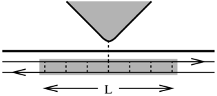
FIG. 3.: A compound contact. Edge impurity scattering allows for equilibration between the different edge channels within a distance $L$ of the contact, as indicated by the shaded region.

A four terminal Hall conductance measured with such “compound” contacts will be appropriately quantized, when $L>>\ell$. Within the scattering region of size $L$ at the compound current contacts there may be a nonequilibrium current distribution, with $J_{\sigma}\neq 0$. However, they decay away in a distance $\ell$, and at the voltage contacts $J_{\sigma}=0$. The voltage probes will then measure $\mu=J_{\rho}/\nu$, giving a quantized Hall conductance.

One may also consider a compound contact made from a tunnel junction line contact. In this case, solving the kinetic equation shows that when $L>>\ell$, the edge is fully equilibrated at the chemical potential of the “upstream” lead. (Here “upstream” is defined in terms of the direction of propagation of the charge). Thus, the compound line junction contact is an explicit realization of the Büttiker ideal contact even when $p_{2}<0$. The two terminal conductance measured with such contacts should be appropriately quantized.

IV Experimental Implications: Lack of Equlibration for $\nu=4/5,4/3$

In this section we focus on specific predictions regarding edge state equilibration in the FQHE which would be interesting to test experimentally.

In section IIIC we found for filling fractions with $|p_{2}|\geq 4$ (such as $\nu=4/5$ or $4/3$) that the edge state equilibration length diverges at low temperatures. This should lead to a breakdown of the quantization of the Hall conductance as the temperature is lowered.

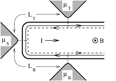
FIG. 4.: Measurement geometry to probe edge state equilibration. Current is injected through the source contact, and the Hall voltage is measured between the contacts $T$ and $B$. As indicated by the solid line, charge propagates counterclockwise along the edge. For $p_{2}<0$, the neutral mode propagates (and decays) in the opposite direction, as indicated by the dashed line. For $p_{2}>0$ the neutral mode propagates clockwise, and the arrow on the dashed line should be reversed.

In order to probe the equilibration between edge states, consider the sample geometry shown in Fig. 4. Current is injected through a source contact, and the Hall voltage is measured using voltage probes on the top and bottom edges at distances $L_{T}$ and $L_{B}$ from the source. We assume that the drain contact is much further away, so that it has no effect on the equilibrium of the edge channels near the voltage probes. For simplicity, as in section 3B1, we model the contacts as tunnel junction point contacts with conductances $G_{Ta},G_{Ba}\ll G_{Sa}$. Further, suppose that the magnetic field points out of the page in Fig. 4, so that that the direction of propagation of the charge $J_{\rho}$ around the edge is counter-clockwise.

Since the source contact is non ideal, it populates the edge modes out of equilibrium. For $\nu=4/3$ ($p_{2}>0$), all of the channels propagate counter clockwise, so that only the top edge is out of equilibrium. The lack of equilibrium on the top edge, characterized by $J_{T\sigma}$, is determined by $I$ and decays away in an equilibration length $\ell$. Following the analysis of section 3B1, we then find that just above the source lead $J_{T\sigma}(0)=(G_{2S}/G_{1S})I$. It then follows that the measured Hall voltage is not quantized, and is given by

$$\mu_{T}-\mu_{B}={h\over e}\left({1\over\nu}+{G_{2T}G_{2S}\over{p_{2}G_{1T}G_{1S}}}e^{-L_{T}/\ell}\right)I,$$ (77)

where $\ell$ is the temperature dependent equilibration length (3.48). Since $G_{2}$ in (4.1) can be either positive or negative, even the sign of the deviation from quantization is non universal. Note that since the bottom edge is fully equilibrated, the nonuniversal linear Hall voltage is independent of the position $L_{B}$ of the bottom contact.

When $\nu=4/5$ ($p_{2}<0$), the neutral mode, $J_{\sigma}$ propagates clockwise, in the opposite direction as $J_{\rho}$. It follows that in this case the bottom edge is out of equilibrium, wheras the top edge is fully equilibrated. The measured linear Hall voltage is given by (4.1) with T replaced by B. Surprisingly, even though the current is injected onto the top edge, the nonuniversal linear Hall voltage depends only on the position $L_{B}$ of the bottom contact.

In order to estimate the temperature at which the lack of equilibration should be detectable, let us consider the temperature scale $T^{*}$ at which the equilibration length is comparable to the distance $L$ between contacts. ¿From (3.48),

$$T^{*}=T_{0}\left({\ell_{0}\over L}\right)^{1/\alpha}.$$ (78)

As a rough estimate we take the cutoff energy $T_{0}$ to be equal the excitation gap for the bulk Hall fluid, $T_{0}\approx 1^{\circ}{\rm K}$. For $\nu=4/5$, the tunneling length in the absence of any effects due to quantum coherence, $\ell_{0}$, depends on the impurity concentration near the edge and the physical separation between the two channels. With the rough estimate, $\ell_{0}\approx 10{\rm nm}$, and with $L=1\mu{\rm m}$ and $\alpha=2$, this gives a crossover temperature, $T^{*}\approx 100{\rm mK}$. For $\nu=4/3$, however, the two channels reside in different Landau levels. Since the Zeeman energy is significantly less than the cyclotron energy, the two channels will have opposite spin. It follows that inter-channel scattering can only occur via spin-orbit or spin flip scattering. The bare tunneling length $\ell_{0}$ should therefore be substantially longer than for $\nu=4/5$, and $T^{*}$ substantially higher.

For temperatures $T>T^{*}$, the neutral current $J_{\sigma}$ decays essentially to zero between the leads, and the edge channels effectively equilibrate, resulting in a quantized conductance. For $T<T^{*}$, however, full equilibration does not take place between the contacts and a non-universal Hall conductance given by (4.1) is expected.

While a non-universal linear conductance is expected at low temperatures, we now argue that increasing the voltage can restore the quantization. In the following we consider the case $\nu=4/3$. The results for $\nu=4/5$ are obtained, as above, by interchanging T and B. At zero temperature, $J_{T\sigma}$ decays according to (3.51) due to the non-ohmic interchannel tunneling.

$$J_{T\sigma}(L_{T})={J_{T\sigma}(0)\over{\left[1+(c_{S}I/I^{*})^{\alpha}\right]^{1/\alpha}}}$$ (79)

where $c_{S}=\alpha^{1/\alpha}G_{2S}/G_{1S}$. Here, the characteristic current,

$$I^{*}={ek_{B}T_{0}\over h}\left({\ell_{0}\over L_{T}}\right)^{1/\alpha}={ek_{B}T^{*}\over h},$$ (80)

sets the scale for the size of the linear response regime. Using the above estimates we find $I^{*}\approx.5{\rm nA}$.

For $I<I^{*}$ there is no significant decay in the neutral current $J_{\sigma}$, by the time it reaches the top voltage contact, and the linear conductance is not quantized. However, at higher currents, the inter-channel equilibration is enhanced by nonlinear tunneling. For $I\gg I^{*}$, the neutral current at the top voltage contact is $J_{T\sigma}(L)=\alpha^{-1/\alpha}I^{*}$. In this regime, the measured Hall voltage may be deduced from (3.38).

$$\mu_{T}-\mu_{B}={h\over\nu e}\left(I+d_{T}I^{*}\right),$$ (81)

where $d_{T}=\alpha^{-1/\alpha}\nu G_{2T}/p_{2}G_{1T}$. This predicts a quantized Hall resistance when the source-drain current $I$ is much larger than $I^{*}$. However, deviations from the quantized value, of order $I^{*}/I$, are present as a result of the incomplete equilibration between the two edge modes. These deviations lead to a slight offset of the linear I-V characteristic at high currents. The constant $d_{T}$, which can be of order $1$, depends on the structure of the voltage contact, and can be either positive or negative.

V Conclusion

As is well known in the integer quantum Hall effect, equilibration between mulitple channels on the same edge is a prerequisite for quantization of the Hall conductance. There are two sources for this equilibration: Edge impurity scattering, and equilibration at the electrical contacts. In the IQHE these can be analyzed using a free-electron model of the edge modes. In this paper, we have generalized to the FQHE, introducing a simple kinetic equation description of FQHE edge dynamics. This approach allows for a unified analysis of equilibration due to both electrical contacts and edge impurity scattering. More specifically, we have introduced and analyzed several concrete models for electrical contacts in the FQHE regime. This allows us to describe realistic transport geometries with multiple current and voltage contacts.

The important new feature which distinguishes FQHE edge dynamics from the IQHE, is the presence of edge modes which move in both directions along the edge, such as for filling $\nu=2/3$. In this case, it is very difficult to equilibrate at the electrical contacts, as we have seen in detail by considering various specific models. Rather, equilibration requires direct inter-channel charge transfer, from edge impurity scattering. This is in contrast with the IQHE, for which multiple channels moving in the same direction can readily be brought into equilibrium by an electrical contact. Surprisingly, for certain quantum Hall states, notably $\nu=4/5$ and $\nu=4/3$, the length scale for equilibration between the edge channels due to impurity scattering diverges at low temperatures. This results in a breakdown of quantization for the Hall conductance at low temperatures in small samples.

We hope that this work will help stimulate further experimental exploration of mesoscopic phenomena in the fractional quantum Hall regime.

- [1] See, for example, Mesoscopic Phenomena in Solids, edited by B. L. Altshuler, P.A. Lee and R.A. Webb (Elsevier, Amsterdam, 1990).
- [2] M. Büttiker, Phys. Rev. B 38, 9375 (1988).
- [3] R. Landauer, Phil. Mag. 21, 863 (1970).
- [4] B.W. Alphenaar, P.L. McEuen, R.G. Wheeler and R.N. Sacks, Phys. Rev. Lett. 64, 677 (1990).
- [5] L.P. Kouwenhoven, et. al. Phys. Rev. Lett. 64, 685 (1990).
- [6] Y. Takagaki, et. al. Phys. Rev. B 50, 4456 (1994).
- [7] X.G. Wen, Phys. Rev. B 43, 11025 (1991); Phys. Rev. Lett. 64, 2206 (1990).
- [8] C.L. Kane, M.P.A. Fisher and J. Polchinski, Phys. Rev. Lett. 72, 4129 (1994).
- [9] C.L. Kane and M.P.A. Fisher, Phys. Rev. B 51 13449, (1995).
- [10] F.D.M. Haldane, Phys. Rev. Lett. 74, 2090 (1995);
- [11] F.D.M. Haldane, Phys. Rev. Lett. 51, 605 (1983); B.I. Halperin, Phys. Rev. Lett. 52, 1583 (1984).
- [12] See, e.g. D. Pines and P. Nozieres, “The Theory of Quantum Liquids,” Benjamin 1966.
- [13] D.S. Fisher and P.A. Lee, Phys. Rev. B 23, 6851 (1981).
- [14] H.U. Baranger and A.D. Stone, Phys. Rev. B 40, 8169 (1989).
- [15] B.I. Halperin, Phys. Rev. B 25, 2185 (1982).
- [16] N. Read, Phys. Rev. Lett. 65, 1502 (1990).
- [17] X.G. Wen and A. Zee, Phys. Rev. B 46, 2290 (1992).
- [18] We thank B.I. Halperin for suggesting the compound contact to us.