Spectral Correlation and Response functions in Quantum Dots

Abstract

We derive a general relation between correlators of density of states fluctuations and density response functions. It applies equally to quantum chaotic systems of pure symmetry (unitary, orthogonal, and symplectic) as well as to the crossover region between the universality classes. This relation is much more robust than Wigner-Dyson statistics; its validity extends to disordered metals with finite conductance and even to the Anderson insulators with large localization length.

One way to investigate a many-body system is to measure its response to an external perturbation. The response functions to which these measurements correspond can be presented through the two-particle Green function. In this Letter, we obtain and discuss generic properties of the response functions of quantum chaotic systems focusing particular attention on the behavior of disordered metallic grains (quantum dots). The exact analytical results which we obtain apply beyond the universal regime described by the random matrix theory.

Chaotic quantum dots and chaotic quantum systems in general are known to exhibit a large degree of universality. Typically, this has been demonstrated by focusing on the statistical properties of spectra. Perhaps the most widely studied statistical characteristic is the two-point correlator of density of states (DoS) fluctuations $R_{2}(\omega)$ [2, 3]. Measuring the probability of finding an eigenstate at a distance $\omega$ in energy from a given state, it illustrates clearly such features as the repulsion of energy levels, spectral rigidity, etc. In particular, for disordered metallic systems, an expression for $R_{2}(\omega)$ can be determined explicitly [4, 5] and compared with the result from the random matrix theory. Recently the correlator was generalized to account for spectra that disperse as a function of some external tunable parameter [6, 7, 8, 9, 10]. The parametric two-point correlator of DoS expresses the probability to find two states separated by an amount $\omega$ and $x$ in energy and parameter space respectively.

$R_{2}(\omega)$ provides just one example of a two-particle average Green function. Others which describe responses of the system to external perturbations involve the structure of the eigenfunctions through matrix elements in addition to spectral properties. However, the striking feature to emerge from recent studies is the observation that the different response Green functions are, in fact, not independent, but connected by a set of differential relations (see Ref. [11], and below). In this Letter, we will investigate the origin of these relations. Doing so, we will demonstrate that, for disordered quantum dots, these relations can be substantially generalized to encompass the non-universal regime of finite dimensionless conductance $g$. The exact analytical relations we derive apply beyond random matrix theory, where analytical expressions for different correlators are as yet unknown. Indeed the results are valid even when the states are localized provided the localization length is sufficiently large.

To make our discussion concrete, we focus on the problem of a quantum dot subject to an external perturbation $\Phi$ whose strength is controlled by a parameter $X$,

$$H(X)={1\over 2m}\left(\mathchoice{{\hbox{\boldmath$\displaystyle p$}}}{{\hbox{\boldmath$\textstyle p$}}}{{\hbox{\boldmath$\scriptstyle p$}}}{{\hbox{\boldmath$\scriptscriptstyle p$}}}-{e\over c}\mathchoice{{\hbox{\boldmath$\displaystyle A$}}}{{\hbox{\boldmath$\textstyle A$}}}{{\hbox{\boldmath$\scriptstyle A$}}}{{\hbox{\boldmath$\scriptscriptstyle A$}}}\right)^{2}+U(\mathchoice{{\hbox{\boldmath$\displaystyle r$}}}{{\hbox{\boldmath$\textstyle r$}}}{{\hbox{\boldmath$\scriptstyle r$}}}{{\hbox{\boldmath$\scriptscriptstyle r$}}})+X\Phi(\mathchoice{{\hbox{\boldmath$\displaystyle r$}}}{{\hbox{\boldmath$\textstyle r$}}}{{\hbox{\boldmath$\scriptstyle r$}}}{{\hbox{\boldmath$\scriptscriptstyle r$}}}).$$ (1)

The random impurity potential $U(\mathchoice{{\hbox{\boldmath$\displaystyle r$}}}{{\hbox{\boldmath$\textstyle r$}}}{{\hbox{\boldmath$\scriptstyle r$}}}{{\hbox{\boldmath$\scriptscriptstyle r$}}})$ is taken to be $\delta$-correlated white-noise with $\langle U(\mathchoice{{\hbox{\boldmath$\displaystyle r$}}}{{\hbox{\boldmath$\textstyle r$}}}{{\hbox{\boldmath$\scriptstyle r$}}}{{\hbox{\boldmath$\scriptscriptstyle r$}}})U(\mathchoice{{\hbox{\boldmath$\displaystyle r$}}}{{\hbox{\boldmath$\textstyle r$}}}{{\hbox{\boldmath$\scriptstyle r$}}}{{\hbox{\boldmath$\scriptscriptstyle r$}}}^{\prime})\rangle=\delta(\mathchoice{{\hbox{\boldmath$\displaystyle r$}}}{{\hbox{\boldmath$\textstyle r$}}}{{\hbox{\boldmath$\scriptstyle r$}}}{{\hbox{\boldmath$\scriptscriptstyle r$}}}-\mathchoice{{\hbox{\boldmath$\displaystyle r$}}}{{\hbox{\boldmath$\textstyle r$}}}{{\hbox{\boldmath$\scriptstyle r$}}}{{\hbox{\boldmath$\scriptscriptstyle r$}}}^{\prime})/2\pi\nu\tau$, where $\nu$ denotes the average DoS and $\tau$ is the relaxation time. A vector potential $\textstyle A$ is included in the unperturbed Hamiltonian and allows an interpolation between orthogonal (T-invariant) and unitary (broken T-invariant) symmetry. The perturbation $\Phi(\mathchoice{{\hbox{\boldmath$\displaystyle r$}}}{{\hbox{\boldmath$\textstyle r$}}}{{\hbox{\boldmath$\scriptstyle r$}}}{{\hbox{\boldmath$\scriptscriptstyle r$}}})$ is assumed to be local by comparison with the mean free path $\ell$, and to preserve the generic (spin-rotation/ time-reversal) symmetries of the Hamiltonian $H(X=0)$.

The response of the metallic grain to the external perturbation is embodied in the two-particle Green function. The separation of fast and slowly varying modes (see below) allow the contributions to this average to be separated into three parts defined by three spatially dependent functions $k$, $n_{D}$ and $n_{C}$ (Fig. 1):

$${1\over 2\pi^{2}\nu^{2}}\left[\left\langle{G^{A}_{E_{1}X_{1}}(\mathchoice{{\hbox{\boldmath$\displaystyle r$}}}{{\hbox{\boldmath$\textstyle r$}}}{{\hbox{\boldmath$\scriptstyle r$}}}{{\hbox{\boldmath$\scriptscriptstyle r$}}}_{1},\mathchoice{{\hbox{\boldmath$\displaystyle r$}}}{{\hbox{\boldmath$\textstyle r$}}}{{\hbox{\boldmath$\scriptstyle r$}}}{{\hbox{\boldmath$\scriptscriptstyle r$}}}_{2})\,G^{R}_{E_{2}X_{2}}(\mathchoice{{\hbox{\boldmath$\displaystyle r$}}}{{\hbox{\boldmath$\textstyle r$}}}{{\hbox{\boldmath$\scriptstyle r$}}}{{\hbox{\boldmath$\scriptscriptstyle r$}}}_{3},\mathchoice{{\hbox{\boldmath$\displaystyle r$}}}{{\hbox{\boldmath$\textstyle r$}}}{{\hbox{\boldmath$\scriptstyle r$}}}{{\hbox{\boldmath$\scriptscriptstyle r$}}}_{4})}\right\rangle-G_{0}^{A}(r_{12})G_{0}^{R}(r_{34})\right]$$ (2)

$$\quad=f(r_{12})f(r_{34})\;k(\mathchoice{{\hbox{\boldmath$\displaystyle R$}}}{{\hbox{\boldmath$\textstyle R$}}}{{\hbox{\boldmath$\scriptstyle R$}}}{{\hbox{\boldmath$\scriptscriptstyle R$}}}_{12},\mathchoice{{\hbox{\boldmath$\displaystyle R$}}}{{\hbox{\boldmath$\textstyle R$}}}{{\hbox{\boldmath$\scriptstyle R$}}}{{\hbox{\boldmath$\scriptscriptstyle R$}}}_{34};\Omega,X)+f(r_{23})f(r_{41})\;n_{D}(\mathchoice{{\hbox{\boldmath$\displaystyle R$}}}{{\hbox{\boldmath$\textstyle R$}}}{{\hbox{\boldmath$\scriptstyle R$}}}{{\hbox{\boldmath$\scriptscriptstyle R$}}}_{23},\mathchoice{{\hbox{\boldmath$\displaystyle R$}}}{{\hbox{\boldmath$\textstyle R$}}}{{\hbox{\boldmath$\scriptstyle R$}}}{{\hbox{\boldmath$\scriptscriptstyle R$}}}_{14};\Omega,X)$$ (3)

$$\qquad+f(r_{24})f(r_{13})\;n_{C}(\mathchoice{{\hbox{\boldmath$\displaystyle R$}}}{{\hbox{\boldmath$\textstyle R$}}}{{\hbox{\boldmath$\scriptstyle R$}}}{{\hbox{\boldmath$\scriptscriptstyle R$}}}_{24},\mathchoice{{\hbox{\boldmath$\displaystyle R$}}}{{\hbox{\boldmath$\textstyle R$}}}{{\hbox{\boldmath$\scriptstyle R$}}}{{\hbox{\boldmath$\scriptscriptstyle R$}}}_{13};\Omega,X),$$ (4)

where $G^{R,A}_{E,X}(\mathchoice{{\hbox{\boldmath$\displaystyle r$}}}{{\hbox{\boldmath$\textstyle r$}}}{{\hbox{\boldmath$\scriptstyle r$}}}{{\hbox{\boldmath$\scriptscriptstyle r$}}}_{1},\mathchoice{{\hbox{\boldmath$\displaystyle r$}}}{{\hbox{\boldmath$\textstyle r$}}}{{\hbox{\boldmath$\scriptstyle r$}}}{{\hbox{\boldmath$\scriptscriptstyle r$}}}_{2})=\langle\mathchoice{{\hbox{\boldmath$\displaystyle r$}}}{{\hbox{\boldmath$\textstyle r$}}}{{\hbox{\boldmath$\scriptstyle r$}}}{{\hbox{\boldmath$\scriptscriptstyle r$}}}_{1}|(E-H(X)\pm i0)^{-1}|\mathchoice{{\hbox{\boldmath$\displaystyle r$}}}{{\hbox{\boldmath$\textstyle r$}}}{{\hbox{\boldmath$\scriptstyle r$}}}{{\hbox{\boldmath$\scriptscriptstyle r$}}}_{2}\rangle$ denotes the Green function, $\Omega=E_{2}-E_{1}$, $X=X_{2}-X_{1}$, $r_{ij}=|\mathchoice{{\hbox{\boldmath$\displaystyle r$}}}{{\hbox{\boldmath$\textstyle r$}}}{{\hbox{\boldmath$\scriptstyle r$}}}{{\hbox{\boldmath$\scriptscriptstyle r$}}}_{i}-\mathchoice{{\hbox{\boldmath$\displaystyle r$}}}{{\hbox{\boldmath$\textstyle r$}}}{{\hbox{\boldmath$\scriptstyle r$}}}{{\hbox{\boldmath$\scriptscriptstyle r$}}}_{j}|$, and $\mathchoice{{\hbox{\boldmath$\displaystyle R$}}}{{\hbox{\boldmath$\textstyle R$}}}{{\hbox{\boldmath$\scriptstyle R$}}}{{\hbox{\boldmath$\scriptscriptstyle R$}}}_{ij}=(\mathchoice{{\hbox{\boldmath$\displaystyle r$}}}{{\hbox{\boldmath$\textstyle r$}}}{{\hbox{\boldmath$\scriptstyle r$}}}{{\hbox{\boldmath$\scriptscriptstyle r$}}}_{i}+\mathchoice{{\hbox{\boldmath$\displaystyle r$}}}{{\hbox{\boldmath$\textstyle r$}}}{{\hbox{\boldmath$\scriptstyle r$}}}{{\hbox{\boldmath$\scriptscriptstyle r$}}}_{j})/2$, and $\langle\cdots\rangle$ represents the ensemble average. The normalized Friedel function is defined by $f(r)=\mbox{Im}\,G^{A}_{0}(r)/\mbox{Im}\,G^{A}_{0}(0)$ where $G^{R,A}_{0}(r_{12})=\langle G^{R,A}_{E,X}(\mathchoice{{\hbox{\boldmath$\displaystyle r$}}}{{\hbox{\boldmath$\textstyle r$}}}{{\hbox{\boldmath$\scriptstyle r$}}}{{\hbox{\boldmath$\scriptscriptstyle r$}}}_{1},\mathchoice{{\hbox{\boldmath$\displaystyle r$}}}{{\hbox{\boldmath$\textstyle r$}}}{{\hbox{\boldmath$\scriptstyle r$}}}{{\hbox{\boldmath$\scriptscriptstyle r$}}}_{2})\rangle$ denotes the average Green function. For a $d$-dimensional system, $f(r)$ can be presented as a Bessel function,

$\displaystyle f(r)=\Gamma(d/2)(2/k_{F}r)^{d/2-1}J_{d/2-1}(k_{F}r)\,e^{-r/2\ell}.$

We remark that our notation for the functions $n_{D}$ and $n_{C}$ is chosen to distinguish the Diffuson from the Cooperon-type contributions (Fig. 1). The decomposition implied by Eq. (4) relies on the rapid decay of $f(r)$ on a scale comparable to the wavelength $k_{F}^{-1}\ll\ell$. Since the typical length scale of $k$ and $n_{D,C}$ is the system size $L$, or the localization length $\xi$, Eq. (4) is applicable not only when the electronic states are extended, but even when they are localized, provided that $L,\xi\gg\ell$.

If the symmetry of the Hamiltonian itself is unchanged by the perturbation $\Phi$, and $H(X)$ belongs to one of the Dyson ensembles (pure symmetry cases), then $n_{C}=n_{D}$ for the systems in which T-invariance is conserved (orthogonal or symplectic class), while $n_{C}=0$ for systems in which T-invariance is violated (unitary class). Therefore, according to Eq. (4), for pure symmetries, all the statistical properties of the two-particle Green function are embodied in the two functions, $k$ and $n\equiv n_{D}$. However, remarkably they are not independent of each other. In particular, we will show that they are connected by the relation

$$\int\!\!d\mathchoice{{\hbox{\boldmath$\displaystyle r$}}}{{\hbox{\boldmath$\textstyle r$}}}{{\hbox{\boldmath$\scriptstyle r$}}}{{\hbox{\boldmath$\scriptscriptstyle r$}}}_{1}d\mathchoice{{\hbox{\boldmath$\displaystyle r$}}}{{\hbox{\boldmath$\textstyle r$}}}{{\hbox{\boldmath$\scriptstyle r$}}}{{\hbox{\boldmath$\scriptscriptstyle r$}}}_{2}\left[2{\partial\over\partial X^{2}}+\left({\Phi(\mathchoice{{\hbox{\boldmath$\displaystyle r$}}}{{\hbox{\boldmath$\textstyle r$}}}{{\hbox{\boldmath$\scriptstyle r$}}}{{\hbox{\boldmath$\scriptscriptstyle r$}}}_{1})+\Phi(\mathchoice{{\hbox{\boldmath$\displaystyle r$}}}{{\hbox{\boldmath$\textstyle r$}}}{{\hbox{\boldmath$\scriptstyle r$}}}{{\hbox{\boldmath$\scriptscriptstyle r$}}}_{2})\over 2X}\right){\partial\over\partial\Omega}\right]k(\mathchoice{{\hbox{\boldmath$\displaystyle r$}}}{{\hbox{\boldmath$\textstyle r$}}}{{\hbox{\boldmath$\scriptstyle r$}}}{{\hbox{\boldmath$\scriptscriptstyle r$}}}_{1},\mathchoice{{\hbox{\boldmath$\displaystyle r$}}}{{\hbox{\boldmath$\textstyle r$}}}{{\hbox{\boldmath$\scriptstyle r$}}}{{\hbox{\boldmath$\scriptscriptstyle r$}}}_{2};\Omega,X)$$ (5)

$$\qquad={\partial^{2}\over\partial\Omega^{2}}\int\!\!d\mathchoice{{\hbox{\boldmath$\displaystyle r$}}}{{\hbox{\boldmath$\textstyle r$}}}{{\hbox{\boldmath$\scriptstyle r$}}}{{\hbox{\boldmath$\scriptscriptstyle r$}}}\,\varphi(\mathchoice{{\hbox{\boldmath$\displaystyle r$}}}{{\hbox{\boldmath$\textstyle r$}}}{{\hbox{\boldmath$\scriptstyle r$}}}{{\hbox{\boldmath$\scriptscriptstyle r$}}})\;\left[n_{D}(\mathchoice{{\hbox{\boldmath$\displaystyle r$}}}{{\hbox{\boldmath$\textstyle r$}}}{{\hbox{\boldmath$\scriptstyle r$}}}{{\hbox{\boldmath$\scriptscriptstyle r$}}},\mathchoice{{\hbox{\boldmath$\displaystyle r$}}}{{\hbox{\boldmath$\textstyle r$}}}{{\hbox{\boldmath$\scriptstyle r$}}}{{\hbox{\boldmath$\scriptscriptstyle r$}}};\Omega,X)+n_{C}(\mathchoice{{\hbox{\boldmath$\displaystyle r$}}}{{\hbox{\boldmath$\textstyle r$}}}{{\hbox{\boldmath$\scriptstyle r$}}}{{\hbox{\boldmath$\scriptscriptstyle r$}}},\mathchoice{{\hbox{\boldmath$\displaystyle r$}}}{{\hbox{\boldmath$\textstyle r$}}}{{\hbox{\boldmath$\scriptstyle r$}}}{{\hbox{\boldmath$\scriptscriptstyle r$}}};\Omega,X)\right],$$ (6)

where

$$\varphi(\mathchoice{{\hbox{\boldmath$\displaystyle r$}}}{{\hbox{\boldmath$\textstyle r$}}}{{\hbox{\boldmath$\scriptstyle r$}}}{{\hbox{\boldmath$\scriptscriptstyle r$}}})=\int\!\!d\mathchoice{{\hbox{\boldmath$\displaystyle r$}}}{{\hbox{\boldmath$\textstyle r$}}}{{\hbox{\boldmath$\scriptstyle r$}}}{{\hbox{\boldmath$\scriptscriptstyle r$}}}_{1}d\mathchoice{{\hbox{\boldmath$\displaystyle r$}}}{{\hbox{\boldmath$\textstyle r$}}}{{\hbox{\boldmath$\scriptstyle r$}}}{{\hbox{\boldmath$\scriptscriptstyle r$}}}_{2}\Phi(\mathchoice{{\hbox{\boldmath$\displaystyle r$}}}{{\hbox{\boldmath$\textstyle r$}}}{{\hbox{\boldmath$\scriptstyle r$}}}{{\hbox{\boldmath$\scriptscriptstyle r$}}}_{1})f^{2}(r_{12})\Phi(\mathchoice{{\hbox{\boldmath$\displaystyle r$}}}{{\hbox{\boldmath$\textstyle r$}}}{{\hbox{\boldmath$\scriptstyle r$}}}{{\hbox{\boldmath$\scriptscriptstyle r$}}}_{2})\;\delta(\mathchoice{{\hbox{\boldmath$\displaystyle r$}}}{{\hbox{\boldmath$\textstyle r$}}}{{\hbox{\boldmath$\scriptstyle r$}}}{{\hbox{\boldmath$\scriptscriptstyle r$}}}-{\mathchoice{{\hbox{\boldmath$\displaystyle r$}}}{{\hbox{\boldmath$\textstyle r$}}}{{\hbox{\boldmath$\scriptstyle r$}}}{{\hbox{\boldmath$\scriptscriptstyle r$}}}_{1}+\mathchoice{{\hbox{\boldmath$\displaystyle r$}}}{{\hbox{\boldmath$\textstyle r$}}}{{\hbox{\boldmath$\scriptstyle r$}}}{{\hbox{\boldmath$\scriptscriptstyle r$}}}_{2}\over 2}).$$ (7)

Eq. (6) represents the main result of the paper. Its range of validity ($\Omega\tau,X\Phi\tau\ll 1$) encompasses a wide interval from the quantum chaotic regime on one hand to the localized phase on the other. It implies strong constraints on the properties of disordered metals in regions where little is known about the explicit form of $k$ and $n$.

In confined or “zero-dimensional” cases where $g\to\infty$ and the coordinate dependence of $k$ and $n$ can be neglected (the random matrix limit), it makes sense to discuss the volume averaged counterparts,

$\displaystyle\left\{\begin{array}[]{cc}k(\Omega,X)\\ n_{D,C}(\Omega,X)\end{array}\right\}=\int{d\mathchoice{{\hbox{\boldmath$\displaystyle r$}}}{{\hbox{\boldmath$\textstyle r$}}}{{\hbox{\boldmath$\scriptstyle r$}}}{{\hbox{\boldmath$\scriptscriptstyle r$}}}_{1}d\mathchoice{{\hbox{\boldmath$\displaystyle r$}}}{{\hbox{\boldmath$\textstyle r$}}}{{\hbox{\boldmath$\scriptstyle r$}}}{{\hbox{\boldmath$\scriptscriptstyle r$}}}_{2}\over V^{2}}\left\{\begin{array}[]{cc}k(\mathchoice{{\hbox{\boldmath$\displaystyle r$}}}{{\hbox{\boldmath$\textstyle r$}}}{{\hbox{\boldmath$\scriptstyle r$}}}{{\hbox{\boldmath$\scriptscriptstyle r$}}}_{1},\mathchoice{{\hbox{\boldmath$\displaystyle r$}}}{{\hbox{\boldmath$\textstyle r$}}}{{\hbox{\boldmath$\scriptstyle r$}}}{{\hbox{\boldmath$\scriptscriptstyle r$}}}_{2};\Omega,X)\\ n_{D,C}(\mathchoice{{\hbox{\boldmath$\displaystyle r$}}}{{\hbox{\boldmath$\textstyle r$}}}{{\hbox{\boldmath$\scriptstyle r$}}}{{\hbox{\boldmath$\scriptscriptstyle r$}}}_{1},\mathchoice{{\hbox{\boldmath$\displaystyle r$}}}{{\hbox{\boldmath$\textstyle r$}}}{{\hbox{\boldmath$\scriptstyle r$}}}{{\hbox{\boldmath$\scriptscriptstyle r$}}}_{2};\Omega,X)\end{array}\right\}.$

The former is related to the two-point correlator of DoS fluctuations through the identity $R_{2}(\omega)=1+{\rm Re}[k(\omega,0)]$, while the latter represents the two types of density response functions. In the same limit an unfolding of the spectrum ($\omega=\Omega/\Delta$) by the average level spacing $\Delta$, and a rescaling of the perturbation $x^{2}=C(0)X^{2}$, where $C(0)=\Delta^{-2}\langle({\partial E_{\alpha}(X)/\partial X})^{2}\rangle$ lifts the dependence of the correlators on the microscopic details of the Hamiltonian including the nature of the perturbation. This independence is a characteristic of systems which displays quantum chaos, and the universal correlation functions $k(\omega,x)$ and $n_{C,D}(\omega,x)$ can be applied quite generally. In particular, studies of $n_{D,C}$ have been used to investigate the response of chaotic systems, such as the dielectric response in complex periodic crystals, the quantum return probability in quantum dots [12], and the statistics of the oscillator strengths [11]. In the universal limit, a direct evaluation of $k(\omega,x)$ and $n_{D}(\omega,x)$ established the zero-dimensional analogue of Eq. (6) [11].

$$2{\partial\over\partial x^{2}}k(\omega,x)={\partial^{2}\over\partial\omega^{2}}n_{D}(\omega,x),$$ (8)

Note that the linear term of $\Phi$ in Eq. (6) is absent since the average drift of the spectrum is excluded by $\mbox{Tr}\Phi=0$. Since Eq. (8) relies on the statistical independence of wavefunction and spectra statistics, the difference of Eq. (6) and Eq. (8) may imply the presence of the correlation between the wavefunction and the spectra.

A similar result to Eq. (8) is found to apply beyond zero-dimension models when $\Phi$ describes an irregular or random potential with some finite range. Since averaging over $\Phi$ is expected, the linear term of $\Phi$ in Eq. (6) vanishes, and $\varphi(\mathchoice{{\hbox{\boldmath$\displaystyle r$}}}{{\hbox{\boldmath$\textstyle r$}}}{{\hbox{\boldmath$\scriptstyle r$}}}{{\hbox{\boldmath$\scriptscriptstyle r$}}})$ is independent of $\textstyle r$. This contrasts with the case of a Gaussian white noise random potential when the linear term does not vanish. In this case. Eq. (6) generates a relation between the return back probability $P(t)$ defined by

$$P(t)=\int\!\!d\Omega\,e^{-i\Omega t}\langle G^{A}_{E,X}(\mathchoice{{\hbox{\boldmath$\displaystyle r$}}}{{\hbox{\boldmath$\textstyle r$}}}{{\hbox{\boldmath$\scriptstyle r$}}}{{\hbox{\boldmath$\scriptscriptstyle r$}}},\mathchoice{{\hbox{\boldmath$\displaystyle r$}}}{{\hbox{\boldmath$\textstyle r$}}}{{\hbox{\boldmath$\scriptstyle r$}}}{{\hbox{\boldmath$\scriptscriptstyle r$}}})\,G^{R}_{E+\Omega,X}(\mathchoice{{\hbox{\boldmath$\displaystyle r$}}}{{\hbox{\boldmath$\textstyle r$}}}{{\hbox{\boldmath$\scriptstyle r$}}}{{\hbox{\boldmath$\scriptscriptstyle r$}}},\mathchoice{{\hbox{\boldmath$\displaystyle r$}}}{{\hbox{\boldmath$\textstyle r$}}}{{\hbox{\boldmath$\scriptstyle r$}}}{{\hbox{\boldmath$\scriptscriptstyle r$}}})\rangle.$$ (9)

and DoS correlator $k$ [13],

$$2{\partial\over\partial X^{2}}S(t,X=0)=-{V\overline{\varphi}\over 2\pi^{2}}\;t^{2}P(t),$$ (10)

where we introduce the form factor $S(t,X)=\Delta^{-2}\int e^{i\Omega t}k(\Omega,X)d\Omega$.

Finally, before turning to the derivation of Eq. (6), let us examine what the formula implies for the relation between the universal response functions in the crossover region between the universality classes. If a T-invariant Hamiltonian is subject to a perturbation which violates T-invariance, the degrees of freedom which rely on the interference of time-reversed paths — the Cooper channel — are suppressed while the Diffuson channel is unaffected [14]. This is reflected in the different behavior shown by the correlation functions $n_{D}$ and $n_{C}$.

The effect of a symmetry breaking perturbation can be demonstrated by generalizing the Hamiltonian in Eq. (1) to include two types of perturbation:

$$H(X_{o},\mathchoice{{\hbox{\boldmath$\displaystyle X$}}}{{\hbox{\boldmath$\textstyle X$}}}{{\hbox{\boldmath$\scriptstyle X$}}}{{\hbox{\boldmath$\scriptscriptstyle X$}}}_{u})=H_{0}+X_{o}\Phi_{o}+\mathchoice{{\hbox{\boldmath$\displaystyle X$}}}{{\hbox{\boldmath$\textstyle X$}}}{{\hbox{\boldmath$\scriptstyle X$}}}{{\hbox{\boldmath$\scriptscriptstyle X$}}}_{u}\cdot\mathchoice{{\hbox{\boldmath$\displaystyle\Phi$}}}{{\hbox{\boldmath$\textstyle\Phi$}}}{{\hbox{\boldmath$\scriptstyle\Phi$}}}{{\hbox{\boldmath$\scriptscriptstyle\Phi$}}}_{u},$$ (11)

where $\Phi_{o}$ preserves T-invariance, whereas $\mathchoice{{\hbox{\boldmath$\displaystyle\Phi$}}}{{\hbox{\boldmath$\textstyle\Phi$}}}{{\hbox{\boldmath$\scriptstyle\Phi$}}}{{\hbox{\boldmath$\scriptscriptstyle\Phi$}}}_{u}=\{\Phi^{(i)}_{u}\}$ breaks it. Since there are, in principle, many different ways to violate T-invariance, we designate $\mathchoice{{\hbox{\boldmath$\displaystyle\Phi$}}}{{\hbox{\boldmath$\textstyle\Phi$}}}{{\hbox{\boldmath$\scriptstyle\Phi$}}}{{\hbox{\boldmath$\scriptscriptstyle\Phi$}}}_{u}$ as a vector describing different possible perturbations and assume $\mbox{Tr}\ [\Phi_{u}^{(i)}\Phi_{u}^{(j)}]\propto\delta_{ij}$. In general, the two-particle average Green function $\langle G^{R}_{E_{1},X_{o1},\mathchoice{{\hbox{\boldmath$\displaystyle X$}}}{{\hbox{\boldmath$\textstyle X$}}}{{\hbox{\boldmath$\scriptstyle X$}}}{{\hbox{\boldmath$\scriptscriptstyle X$}}}_{u1}}\,G^{A}_{E_{2},X_{o2},\mathchoice{{\hbox{\boldmath$\displaystyle X$}}}{{\hbox{\boldmath$\textstyle X$}}}{{\hbox{\boldmath$\scriptstyle X$}}}{{\hbox{\boldmath$\scriptscriptstyle X$}}}_{u2}}\rangle$ depends, not on each of the many parameters, but only on five: the energy difference, $X_{\beta}=X_{\beta 2}-X_{\beta 1}$ ($\beta=u,o$), $|\mathchoice{{\hbox{\boldmath$\displaystyle\bar{X}$}}}{{\hbox{\boldmath$\textstyle\bar{X}$}}}{{\hbox{\boldmath$\scriptstyle\bar{X}$}}}{{\hbox{\boldmath$\scriptscriptstyle\bar{X}$}}}|=|\mathchoice{{\hbox{\boldmath$\displaystyle X$}}}{{\hbox{\boldmath$\textstyle X$}}}{{\hbox{\boldmath$\scriptstyle X$}}}{{\hbox{\boldmath$\scriptscriptstyle X$}}}_{u2}+\mathchoice{{\hbox{\boldmath$\displaystyle X$}}}{{\hbox{\boldmath$\textstyle X$}}}{{\hbox{\boldmath$\scriptstyle X$}}}{{\hbox{\boldmath$\scriptscriptstyle X$}}}_{u1}|/2$ and an angle $\theta$ specifying the “relative direction,” $\mathchoice{{\hbox{\boldmath$\displaystyle\bar{X}$}}}{{\hbox{\boldmath$\textstyle\bar{X}$}}}{{\hbox{\boldmath$\scriptstyle\bar{X}$}}}{{\hbox{\boldmath$\scriptscriptstyle\bar{X}$}}}\cdot\mathchoice{{\hbox{\boldmath$\displaystyle X$}}}{{\hbox{\boldmath$\textstyle X$}}}{{\hbox{\boldmath$\scriptstyle X$}}}{{\hbox{\boldmath$\scriptscriptstyle X$}}}=|\mathchoice{{\hbox{\boldmath$\displaystyle\bar{X}$}}}{{\hbox{\boldmath$\textstyle\bar{X}$}}}{{\hbox{\boldmath$\scriptstyle\bar{X}$}}}{{\hbox{\boldmath$\scriptscriptstyle\bar{X}$}}}||\mathchoice{{\hbox{\boldmath$\displaystyle X$}}}{{\hbox{\boldmath$\textstyle X$}}}{{\hbox{\boldmath$\scriptstyle X$}}}{{\hbox{\boldmath$\scriptscriptstyle X$}}}|\cos\theta$ [15].

In the universal or random matrix limit, the rescalings

$$x_{o}^{2}=C_{o}(0;0)X_{o}^{2},\>x_{u}^{2}=C_{u}(0;\infty)X_{u}^{2},\>\bar{x}^{2}=C_{u}(0;\infty)\bar{X}^{2}$$

$$C_{\beta}(0;\bar{X})={1\over\Delta^{2}}\left\langle\left({\partial E_{\alpha}/\partial X_{\beta}}\right)^{2}\right\rangle,\quad(\beta=o,u),$$

lead to a generalization of Eq. (8) for the crossover interval between orthogonal and unitary ensembles:

$$\left\{{2{\partial\over{\partial(x_{o}^{2})}}\pm\left[{{\partial\over{\partial(x_{u}^{2})}}-{1\over 4}{\partial\over{\partial(\bar{x}^{2})}}-{\cos\theta\over 2}\left({{1\over{4\bar{x}^{2}}}-{1\over{x_{u}^{2}}}}\right){\partial\over{\partial\cos\theta}}}\right]}\right\}\;k={1\over 2}{{\partial^{2}}\over{\partial\omega^{2}}}n_{D,C}.$$ (13)

Since $k(\omega,x_{o},\bar{x},x_{u},\cos\theta)$ is known explicitly [15], this formula determines the response functions $n_{C}$, $n_{D}$ within the crossover region.

We now outline the main elements involved in the derivation together with that of the decomposition formula of Eq. (4). For brevity we will confine our discussion to the properties of T-invariant systems in which the symmetry is not violated by the perturbation. An extension to the crossover regime can be achieved straightforwardly. Our approach and discussion is based on the field theoretic construction developed to describe the low energy “excitations” or diffusion modes in disordered metals, where statistical properties of two-point correlators are presented through an effective nonlinear $\sigma$-model involving $8\times 8$ supermatrix fields $Q$ [4].

Following the conventions of Ref. [4], the $8\times 8$ supermatrix can be decomposed into $4\times 4$ submatrices $Q^{ab}$ ($a,b=1,2$) which reflect the advanced and retarded subspace. The spatially dependent correlations functions can then be expressed as

$$2k(\mathchoice{{\hbox{\boldmath$\displaystyle r$}}}{{\hbox{\boldmath$\textstyle r$}}}{{\hbox{\boldmath$\scriptstyle r$}}}{{\hbox{\boldmath$\scriptscriptstyle r$}}}_{1},\mathchoice{{\hbox{\boldmath$\displaystyle r$}}}{{\hbox{\boldmath$\textstyle r$}}}{{\hbox{\boldmath$\scriptstyle r$}}}{{\hbox{\boldmath$\scriptscriptstyle r$}}}_{2};\Omega,X)=-1-\left\langle Q^{11}_{33}(\mathchoice{{\hbox{\boldmath$\displaystyle r$}}}{{\hbox{\boldmath$\textstyle r$}}}{{\hbox{\boldmath$\scriptstyle r$}}}{{\hbox{\boldmath$\scriptscriptstyle r$}}}_{1})Q^{22}_{33}(\mathchoice{{\hbox{\boldmath$\displaystyle r$}}}{{\hbox{\boldmath$\textstyle r$}}}{{\hbox{\boldmath$\scriptstyle r$}}}{{\hbox{\boldmath$\scriptscriptstyle r$}}}_{2})\right\rangle_{Q},$$ (15)

$$2n_{D}(\mathchoice{{\hbox{\boldmath$\displaystyle r$}}}{{\hbox{\boldmath$\textstyle r$}}}{{\hbox{\boldmath$\scriptstyle r$}}}{{\hbox{\boldmath$\scriptscriptstyle r$}}}_{1},\mathchoice{{\hbox{\boldmath$\displaystyle r$}}}{{\hbox{\boldmath$\textstyle r$}}}{{\hbox{\boldmath$\scriptstyle r$}}}{{\hbox{\boldmath$\scriptscriptstyle r$}}}_{2};\Omega,X)=-\left\langle Q^{12}_{33}(\mathchoice{{\hbox{\boldmath$\displaystyle r$}}}{{\hbox{\boldmath$\textstyle r$}}}{{\hbox{\boldmath$\scriptstyle r$}}}{{\hbox{\boldmath$\scriptscriptstyle r$}}}_{1})Q^{21}_{33}(\mathchoice{{\hbox{\boldmath$\displaystyle r$}}}{{\hbox{\boldmath$\textstyle r$}}}{{\hbox{\boldmath$\scriptstyle r$}}}{{\hbox{\boldmath$\scriptscriptstyle r$}}}_{2})\right\rangle_{Q},$$ (16)

$$2n_{C}(\mathchoice{{\hbox{\boldmath$\displaystyle r$}}}{{\hbox{\boldmath$\textstyle r$}}}{{\hbox{\boldmath$\scriptstyle r$}}}{{\hbox{\boldmath$\scriptscriptstyle r$}}}_{1},\mathchoice{{\hbox{\boldmath$\displaystyle r$}}}{{\hbox{\boldmath$\textstyle r$}}}{{\hbox{\boldmath$\scriptstyle r$}}}{{\hbox{\boldmath$\scriptscriptstyle r$}}}_{2};\Omega,X)=-\left\langle Q^{12}_{34}(\mathchoice{{\hbox{\boldmath$\displaystyle r$}}}{{\hbox{\boldmath$\textstyle r$}}}{{\hbox{\boldmath$\scriptstyle r$}}}{{\hbox{\boldmath$\scriptscriptstyle r$}}}_{1})Q^{21}_{43}(\mathchoice{{\hbox{\boldmath$\displaystyle r$}}}{{\hbox{\boldmath$\textstyle r$}}}{{\hbox{\boldmath$\scriptstyle r$}}}{{\hbox{\boldmath$\scriptscriptstyle r$}}}_{2})\right\rangle_{Q}.$$ (17)

where the integration is restricted to the manifold on which $Q^{2}=\openone_{8}$ and $\left\langle\cdots\right\rangle_{Q}=\int{DQ\,\left(\cdots\right)}\,e^{-F[Q]}$. The effective action $F[Q]$ is given by

$$F[Q]={\pi\nu\over 8}\int\!\!d\mathchoice{{\hbox{\boldmath$\displaystyle r$}}}{{\hbox{\boldmath$\textstyle r$}}}{{\hbox{\boldmath$\scriptstyle r$}}}{{\hbox{\boldmath$\scriptscriptstyle r$}}}\,\mbox{STr}\left\{D(\nabla Q)^{2}+2i[\Omega-X\Phi(\mathchoice{{\hbox{\boldmath$\displaystyle r$}}}{{\hbox{\boldmath$\textstyle r$}}}{{\hbox{\boldmath$\scriptstyle r$}}}{{\hbox{\boldmath$\scriptscriptstyle r$}}})]{Q\Lambda}\right\}$$ (18)

$$\qquad-{\pi^{2}\nu^{2}\over 16}X^{2}\int\!\!d\mathchoice{{\hbox{\boldmath$\displaystyle r$}}}{{\hbox{\boldmath$\textstyle r$}}}{{\hbox{\boldmath$\scriptstyle r$}}}{{\hbox{\boldmath$\scriptscriptstyle r$}}}\varphi(\mathchoice{{\hbox{\boldmath$\displaystyle r$}}}{{\hbox{\boldmath$\textstyle r$}}}{{\hbox{\boldmath$\scriptstyle r$}}}{{\hbox{\boldmath$\scriptscriptstyle r$}}})\mbox{STr}[Q\Lambda Q\Lambda],$$ (19)

where $D=v_{F}^{2}\tau/d$ denotes the diffusion coefficient, and $\Lambda=\mbox{diag}(\openone_{4},-\openone_{4})$ is the constant matrix that breaks the symmetry between the retarded and advanced Green functions. The explicit structure of $Q$ corresponding to the three universality classes can be found in Ref. [4].

The decomposition formula of Eq. (4) is obtained by presenting the average two-particle Green function in terms of the supermatrix Green functions,

$$\left\langle{G^{A}_{E_{1},X_{1}}(\mathchoice{{\hbox{\boldmath$\displaystyle r$}}}{{\hbox{\boldmath$\textstyle r$}}}{{\hbox{\boldmath$\scriptstyle r$}}}{{\hbox{\boldmath$\scriptscriptstyle r$}}}_{1},\mathchoice{{\hbox{\boldmath$\displaystyle r$}}}{{\hbox{\boldmath$\textstyle r$}}}{{\hbox{\boldmath$\scriptstyle r$}}}{{\hbox{\boldmath$\scriptscriptstyle r$}}}_{2})\,G^{R}_{E_{2},X_{2}}(\mathchoice{{\hbox{\boldmath$\displaystyle r$}}}{{\hbox{\boldmath$\textstyle r$}}}{{\hbox{\boldmath$\scriptstyle r$}}}{{\hbox{\boldmath$\scriptscriptstyle r$}}}_{3},\mathchoice{{\hbox{\boldmath$\displaystyle r$}}}{{\hbox{\boldmath$\textstyle r$}}}{{\hbox{\boldmath$\scriptstyle r$}}}{{\hbox{\boldmath$\scriptscriptstyle r$}}}_{4})}\right\rangle=\left\langle{\cal G}^{11}_{33}(\mathchoice{{\hbox{\boldmath$\displaystyle r$}}}{{\hbox{\boldmath$\textstyle r$}}}{{\hbox{\boldmath$\scriptstyle r$}}}{{\hbox{\boldmath$\scriptscriptstyle r$}}}_{1},\mathchoice{{\hbox{\boldmath$\displaystyle r$}}}{{\hbox{\boldmath$\textstyle r$}}}{{\hbox{\boldmath$\scriptstyle r$}}}{{\hbox{\boldmath$\scriptscriptstyle r$}}}_{2})\,{\cal G}^{22}_{33}(\mathchoice{{\hbox{\boldmath$\displaystyle r$}}}{{\hbox{\boldmath$\textstyle r$}}}{{\hbox{\boldmath$\scriptstyle r$}}}{{\hbox{\boldmath$\scriptscriptstyle r$}}}_{3},\mathchoice{{\hbox{\boldmath$\displaystyle r$}}}{{\hbox{\boldmath$\textstyle r$}}}{{\hbox{\boldmath$\scriptstyle r$}}}{{\hbox{\boldmath$\scriptscriptstyle r$}}}_{4})\right\rangle_{Q}$$ (20)

$$\ +\left\langle{\cal G}^{12}_{33}(\mathchoice{{\hbox{\boldmath$\displaystyle r$}}}{{\hbox{\boldmath$\textstyle r$}}}{{\hbox{\boldmath$\scriptstyle r$}}}{{\hbox{\boldmath$\scriptscriptstyle r$}}}_{1},\mathchoice{{\hbox{\boldmath$\displaystyle r$}}}{{\hbox{\boldmath$\textstyle r$}}}{{\hbox{\boldmath$\scriptstyle r$}}}{{\hbox{\boldmath$\scriptscriptstyle r$}}}_{4})\,{\cal G}^{21}_{33}(\mathchoice{{\hbox{\boldmath$\displaystyle r$}}}{{\hbox{\boldmath$\textstyle r$}}}{{\hbox{\boldmath$\scriptstyle r$}}}{{\hbox{\boldmath$\scriptscriptstyle r$}}}_{3},\mathchoice{{\hbox{\boldmath$\displaystyle r$}}}{{\hbox{\boldmath$\textstyle r$}}}{{\hbox{\boldmath$\scriptstyle r$}}}{{\hbox{\boldmath$\scriptscriptstyle r$}}}_{2})+{\cal G}^{12}_{34}(\mathchoice{{\hbox{\boldmath$\displaystyle r$}}}{{\hbox{\boldmath$\textstyle r$}}}{{\hbox{\boldmath$\scriptstyle r$}}}{{\hbox{\boldmath$\scriptscriptstyle r$}}}_{1},\mathchoice{{\hbox{\boldmath$\displaystyle r$}}}{{\hbox{\boldmath$\textstyle r$}}}{{\hbox{\boldmath$\scriptstyle r$}}}{{\hbox{\boldmath$\scriptscriptstyle r$}}}_{3})\,{\cal G}^{21}_{43}(\mathchoice{{\hbox{\boldmath$\displaystyle r$}}}{{\hbox{\boldmath$\textstyle r$}}}{{\hbox{\boldmath$\scriptstyle r$}}}{{\hbox{\boldmath$\scriptscriptstyle r$}}}_{4},\mathchoice{{\hbox{\boldmath$\displaystyle r$}}}{{\hbox{\boldmath$\textstyle r$}}}{{\hbox{\boldmath$\scriptstyle r$}}}{{\hbox{\boldmath$\scriptscriptstyle r$}}}_{2})\right\rangle_{Q},$$ (21)

(22)

where ${\cal G}=[E-\mathchoice{{\hbox{\boldmath$\displaystyle p$}}}{{\hbox{\boldmath$\textstyle p$}}}{{\hbox{\boldmath$\scriptstyle p$}}}{{\hbox{\boldmath$\scriptscriptstyle p$}}}^{2}/2m-(\Omega-X\Phi)\Lambda/2-iQ/2\tau]^{-1}$. For small values of the parameters, the explicit dependence of ${\cal G}$ on $\Omega$ and $X$ can be neglected. Taking account of the slow variation of $Q(\mathchoice{{\hbox{\boldmath$\displaystyle r$}}}{{\hbox{\boldmath$\textstyle r$}}}{{\hbox{\boldmath$\scriptstyle r$}}}{{\hbox{\boldmath$\scriptscriptstyle r$}}})$, ${\cal G}$ can be separated into fast and slowly varying spatial modes:

$${\cal G}(\mathchoice{{\hbox{\boldmath$\displaystyle r$}}}{{\hbox{\boldmath$\textstyle r$}}}{{\hbox{\boldmath$\scriptstyle r$}}}{{\hbox{\boldmath$\scriptscriptstyle r$}}}_{1},\mathchoice{{\hbox{\boldmath$\displaystyle r$}}}{{\hbox{\boldmath$\textstyle r$}}}{{\hbox{\boldmath$\scriptstyle r$}}}{{\hbox{\boldmath$\scriptscriptstyle r$}}}_{2})\approx G^{A}_{0}(r_{12})+i\pi\nu f(r_{12})[Q(\mathchoice{{\hbox{\boldmath$\displaystyle R$}}}{{\hbox{\boldmath$\textstyle R$}}}{{\hbox{\boldmath$\scriptstyle R$}}}{{\hbox{\boldmath$\scriptscriptstyle R$}}}_{12})-\Lambda].$$ (23)

Substitution of Eqs. (22,23) into Eq. (Spectral Correlation and Response functions in Quantum Dots) leads to Eq. (4).

To obtain Eq. (6), we examine the derivative

$${\partial\over\partial X}k(\Omega,X)=\int\!\!d\mathchoice{{\hbox{\boldmath$\displaystyle r$}}}{{\hbox{\boldmath$\textstyle r$}}}{{\hbox{\boldmath$\scriptstyle r$}}}{{\hbox{\boldmath$\scriptscriptstyle r$}}}d\mathchoice{{\hbox{\boldmath$\displaystyle r$}}}{{\hbox{\boldmath$\textstyle r$}}}{{\hbox{\boldmath$\scriptstyle r$}}}{{\hbox{\boldmath$\scriptscriptstyle r$}}}_{1}d\mathchoice{{\hbox{\boldmath$\displaystyle r$}}}{{\hbox{\boldmath$\textstyle r$}}}{{\hbox{\boldmath$\scriptstyle r$}}}{{\hbox{\boldmath$\scriptscriptstyle r$}}}_{2}\,(\delta k_{1}+\delta k_{2}),$$ (24)

where

$$\delta k_{1}={i\pi\nu\over 8}\left\langle\Phi(\mathchoice{{\hbox{\boldmath$\displaystyle r$}}}{{\hbox{\boldmath$\textstyle r$}}}{{\hbox{\boldmath$\scriptstyle r$}}}{{\hbox{\boldmath$\scriptscriptstyle r$}}})\mbox{STr}[Q(\mathchoice{{\hbox{\boldmath$\displaystyle r$}}}{{\hbox{\boldmath$\textstyle r$}}}{{\hbox{\boldmath$\scriptstyle r$}}}{{\hbox{\boldmath$\scriptscriptstyle r$}}})\Lambda]Q^{11}_{33}(\mathchoice{{\hbox{\boldmath$\displaystyle r$}}}{{\hbox{\boldmath$\textstyle r$}}}{{\hbox{\boldmath$\scriptstyle r$}}}{{\hbox{\boldmath$\scriptscriptstyle r$}}}_{1})Q^{22}_{33}(\mathchoice{{\hbox{\boldmath$\displaystyle r$}}}{{\hbox{\boldmath$\textstyle r$}}}{{\hbox{\boldmath$\scriptstyle r$}}}{{\hbox{\boldmath$\scriptscriptstyle r$}}}_{2})\right\rangle_{Q},$$

$$\delta k_{2}=-{\pi^{2}\nu^{2}X\over 16}\left\langle\varphi(\mathchoice{{\hbox{\boldmath$\displaystyle r$}}}{{\hbox{\boldmath$\textstyle r$}}}{{\hbox{\boldmath$\scriptstyle r$}}}{{\hbox{\boldmath$\scriptscriptstyle r$}}})\mbox{STr}[(Q(\mathchoice{{\hbox{\boldmath$\displaystyle r$}}}{{\hbox{\boldmath$\textstyle r$}}}{{\hbox{\boldmath$\scriptstyle r$}}}{{\hbox{\boldmath$\scriptscriptstyle r$}}})\Lambda)^{2}]Q^{11}_{33}(\mathchoice{{\hbox{\boldmath$\displaystyle r$}}}{{\hbox{\boldmath$\textstyle r$}}}{{\hbox{\boldmath$\scriptstyle r$}}}{{\hbox{\boldmath$\scriptscriptstyle r$}}}_{1})Q^{22}_{33}(\mathchoice{{\hbox{\boldmath$\displaystyle r$}}}{{\hbox{\boldmath$\textstyle r$}}}{{\hbox{\boldmath$\scriptstyle r$}}}{{\hbox{\boldmath$\scriptscriptstyle r$}}}_{2})\right\rangle_{Q}.$$

Since $\delta k_{1}$ is given through $\Phi(\mathchoice{{\hbox{\boldmath$\displaystyle r$}}}{{\hbox{\boldmath$\textstyle r$}}}{{\hbox{\boldmath$\scriptstyle r$}}}{{\hbox{\boldmath$\scriptscriptstyle r$}}})(\delta/\delta\Phi(\mathchoice{{\hbox{\boldmath$\displaystyle r$}}}{{\hbox{\boldmath$\textstyle r$}}}{{\hbox{\boldmath$\scriptstyle r$}}}{{\hbox{\boldmath$\scriptscriptstyle r$}}}))k(\mathchoice{{\hbox{\boldmath$\displaystyle r$}}}{{\hbox{\boldmath$\textstyle r$}}}{{\hbox{\boldmath$\scriptstyle r$}}}{{\hbox{\boldmath$\scriptscriptstyle r$}}}_{1},\mathchoice{{\hbox{\boldmath$\displaystyle r$}}}{{\hbox{\boldmath$\textstyle r$}}}{{\hbox{\boldmath$\scriptstyle r$}}}{{\hbox{\boldmath$\scriptscriptstyle r$}}}_{2};\Omega,X)$, the first term can be recast in the form

$${-1\over 2}\int d\mathchoice{{\hbox{\boldmath$\displaystyle r$}}}{{\hbox{\boldmath$\textstyle r$}}}{{\hbox{\boldmath$\scriptstyle r$}}}{{\hbox{\boldmath$\scriptscriptstyle r$}}}_{1}d\mathchoice{{\hbox{\boldmath$\displaystyle r$}}}{{\hbox{\boldmath$\textstyle r$}}}{{\hbox{\boldmath$\scriptstyle r$}}}{{\hbox{\boldmath$\scriptscriptstyle r$}}}_{2}\left(\Phi(\mathchoice{{\hbox{\boldmath$\displaystyle r$}}}{{\hbox{\boldmath$\textstyle r$}}}{{\hbox{\boldmath$\scriptstyle r$}}}{{\hbox{\boldmath$\scriptscriptstyle r$}}}_{1}){\partial\over\partial E_{1}}-\Phi(\mathchoice{{\hbox{\boldmath$\displaystyle r$}}}{{\hbox{\boldmath$\textstyle r$}}}{{\hbox{\boldmath$\scriptstyle r$}}}{{\hbox{\boldmath$\scriptscriptstyle r$}}}_{2}){\partial\over\partial E_{2}}\right)k(\mathchoice{{\hbox{\boldmath$\displaystyle r$}}}{{\hbox{\boldmath$\textstyle r$}}}{{\hbox{\boldmath$\scriptstyle r$}}}{{\hbox{\boldmath$\scriptscriptstyle r$}}}_{1},\mathchoice{{\hbox{\boldmath$\displaystyle r$}}}{{\hbox{\boldmath$\textstyle r$}}}{{\hbox{\boldmath$\scriptstyle r$}}}{{\hbox{\boldmath$\scriptscriptstyle r$}}}_{2})$$ (25)

$$=-\int d\mathchoice{{\hbox{\boldmath$\displaystyle r$}}}{{\hbox{\boldmath$\textstyle r$}}}{{\hbox{\boldmath$\scriptstyle r$}}}{{\hbox{\boldmath$\scriptscriptstyle r$}}}_{1}d\mathchoice{{\hbox{\boldmath$\displaystyle r$}}}{{\hbox{\boldmath$\textstyle r$}}}{{\hbox{\boldmath$\scriptstyle r$}}}{{\hbox{\boldmath$\scriptscriptstyle r$}}}_{2}\left({\Phi(\mathchoice{{\hbox{\boldmath$\displaystyle r$}}}{{\hbox{\boldmath$\textstyle r$}}}{{\hbox{\boldmath$\scriptstyle r$}}}{{\hbox{\boldmath$\scriptscriptstyle r$}}}_{1})+\Phi(\mathchoice{{\hbox{\boldmath$\displaystyle r$}}}{{\hbox{\boldmath$\textstyle r$}}}{{\hbox{\boldmath$\scriptstyle r$}}}{{\hbox{\boldmath$\scriptscriptstyle r$}}}_{2})\over 2}\right){\partial\over\partial\Omega}k(\mathchoice{{\hbox{\boldmath$\displaystyle r$}}}{{\hbox{\boldmath$\textstyle r$}}}{{\hbox{\boldmath$\scriptstyle r$}}}{{\hbox{\boldmath$\scriptscriptstyle r$}}}_{1},\mathchoice{{\hbox{\boldmath$\displaystyle r$}}}{{\hbox{\boldmath$\textstyle r$}}}{{\hbox{\boldmath$\scriptstyle r$}}}{{\hbox{\boldmath$\scriptscriptstyle r$}}}_{2}).$$ (26)

To calculate $\delta k_{2}$, we work with the symmetrized expression for $k$ and $n_{D,C}$ in the fermion-boson subspace [16],

$$k=-{1\over 2}-{1\over 32}\left\langle\mbox{STr}[k_{s}Q^{11}(\mathchoice{{\hbox{\boldmath$\displaystyle r$}}}{{\hbox{\boldmath$\textstyle r$}}}{{\hbox{\boldmath$\scriptstyle r$}}}{{\hbox{\boldmath$\scriptscriptstyle r$}}}_{1})]\mbox{STr}[k_{s}Q^{22}(\mathchoice{{\hbox{\boldmath$\displaystyle r$}}}{{\hbox{\boldmath$\textstyle r$}}}{{\hbox{\boldmath$\scriptstyle r$}}}{{\hbox{\boldmath$\scriptscriptstyle r$}}}_{2})]\right\rangle,$$ (27)

$$n_{D}+n_{C}={1\over 16}\left\langle\mbox{STr}[k_{s}Q^{12}(\mathchoice{{\hbox{\boldmath$\displaystyle r$}}}{{\hbox{\boldmath$\textstyle r$}}}{{\hbox{\boldmath$\scriptstyle r$}}}{{\hbox{\boldmath$\scriptscriptstyle r$}}}_{1})k_{s}Q^{21}(\mathchoice{{\hbox{\boldmath$\displaystyle r$}}}{{\hbox{\boldmath$\textstyle r$}}}{{\hbox{\boldmath$\scriptstyle r$}}}{{\hbox{\boldmath$\scriptscriptstyle r$}}}_{2})]\right\rangle_{Q},$$ (28)

where $k_{s}=\mbox{diag}(\openone_{2},-\openone_{2})$, and utilize the identity,

$$\left\langle\mbox{STr}[Q^{12}Q^{21}(\mathchoice{{\hbox{\boldmath$\displaystyle r$}}}{{\hbox{\boldmath$\textstyle r$}}}{{\hbox{\boldmath$\scriptstyle r$}}}{{\hbox{\boldmath$\scriptscriptstyle r$}}})]\mbox{STr}[k_{s}Q^{11}(\mathchoice{{\hbox{\boldmath$\displaystyle r$}}}{{\hbox{\boldmath$\textstyle r$}}}{{\hbox{\boldmath$\scriptstyle r$}}}{{\hbox{\boldmath$\scriptscriptstyle r$}}}_{1})]\mbox{STr}[k_{s}Q^{22}(\mathchoice{{\hbox{\boldmath$\displaystyle r$}}}{{\hbox{\boldmath$\textstyle r$}}}{{\hbox{\boldmath$\scriptstyle r$}}}{{\hbox{\boldmath$\scriptscriptstyle r$}}}_{2})]\right\rangle_{Q}$$ (29)

$$=\left\langle\mbox{STr}[Q^{11}(\mathchoice{{\hbox{\boldmath$\displaystyle r$}}}{{\hbox{\boldmath$\textstyle r$}}}{{\hbox{\boldmath$\scriptstyle r$}}}{{\hbox{\boldmath$\scriptscriptstyle r$}}}_{1})]\mbox{STr}[Q^{22}(\mathchoice{{\hbox{\boldmath$\displaystyle r$}}}{{\hbox{\boldmath$\textstyle r$}}}{{\hbox{\boldmath$\scriptstyle r$}}}{{\hbox{\boldmath$\scriptscriptstyle r$}}}_{2})]\mbox{STr}[k_{s}Q^{12}k_{s}Q^{21}(\mathchoice{{\hbox{\boldmath$\displaystyle r$}}}{{\hbox{\boldmath$\textstyle r$}}}{{\hbox{\boldmath$\scriptstyle r$}}}{{\hbox{\boldmath$\scriptscriptstyle r$}}})]\right\rangle_{Q}.$$ (30)

The identity originates from the freedom to choose the fermion or boson field to calculate correlators, i.e., the fermion-boson supersymmetry of the $\sigma$-model. (This property was presented explicitly for the two-point correlator of $Q$-matrices in Ref. [16].) Note that since this fermion-boson symmetry is required to impose the correct normalization, it is present even in the crossover interval between universality classes. Since $\mbox{STr}[Q^{11}]=-\mbox{STr}[Q^{22}]$ by the saddle point condition on the $Q$-matrix, the right hand side of Eq. (30) coincides with the second derivative of $n_{D}+n_{C}$ with respect to $\Omega$. In this way, the second integral over $\delta k_{2}$ can be shown to be equal to the right hand side of Eq. (6).

We emphasize that, since the proof of Eq. (6) relies only on the supermatrix nonlinear $\sigma$-model, it applies with the same generality. This implies that the identity encompasses the behaviors both of the mobility edge as well as in the localized phase.

In conclusion, we have derived and discussed a relation between spectral correlators and response functions in disordered metals which applies over a range which encompasses quantum chaos (random matrix limit), the metallic phase (large conductance) and even the Anderson insulating regime with a large localization length.

We are grateful to A. V. Andreev, and I. V. Lerner for useful discussions. The work of NT and BDS was supported in part by the Joint Services Electronic Program No. DAAL 03-89-0001 and by NSF grant No. DMR 92-14480. BDS is grateful for the support of the Royal Society through a Research Fellowship.

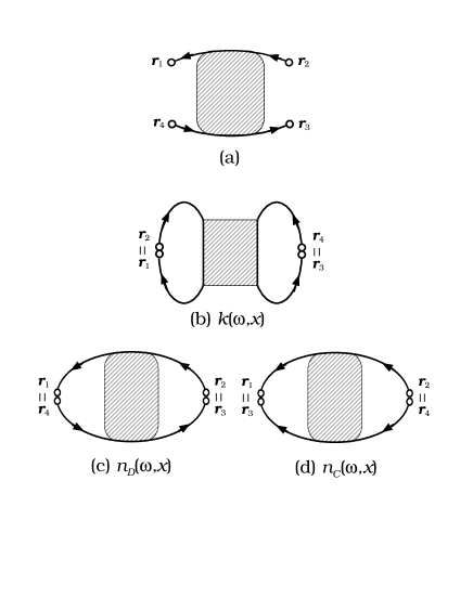
FIG. 1.: (a) Diagram representation of the two-particle Green function $\langle G^{A}(\mathchoice{{\hbox{\boldmath$\displaystyle r$}}}{{\hbox{\boldmath$\textstyle r$}}}{{\hbox{\boldmath$\scriptstyle r$}}}{{\hbox{\boldmath$\scriptscriptstyle r$}}}_{1},\mathchoice{{\hbox{\boldmath$\displaystyle r$}}}{{\hbox{\boldmath$\textstyle r$}}}{{\hbox{\boldmath$\scriptstyle r$}}}{{\hbox{\boldmath$\scriptscriptstyle r$}}}_{2})G^{R}(\mathchoice{{\hbox{\boldmath$\displaystyle r$}}}{{\hbox{\boldmath$\textstyle r$}}}{{\hbox{\boldmath$\scriptstyle r$}}}{{\hbox{\boldmath$\scriptscriptstyle r$}}}_{3},\mathchoice{{\hbox{\boldmath$\displaystyle r$}}}{{\hbox{\boldmath$\textstyle r$}}}{{\hbox{\boldmath$\scriptstyle r$}}}{{\hbox{\boldmath$\scriptscriptstyle r$}}}_{4})\rangle$. (b) DOS fluctuation-type contribution $k$. (c) Cooperon-type contribution $n_{C}$. (d) Diffuson-type contribution $n_{D}$.

REFERENCES

• [1] On leave from Department of Applied Physics, Tokyo University, Tokyo, Japan.
• [2] F. J. Dyson, J. Math. Phys. 3, 140 (1962).
• [3] M. L. Mehta, ‘Random Matrices — Revised and Enlarged Second Edition’ (Academic Press Inc., San Diego, 1991).
• [4] K. B. Efetov, Adv. Phys. 32, 53 (1983).
• [5] J. J. M. Verbaarschot, H. A. Weidenmüller, and M. R. Zirnbauer, Phys. Rep. 129, 367 (1985).
• [6] M. Wilkinson, J. Phys. A 21, 4021 (1988).
• [7] P. Gaspard, S. A. Rice, M. J. Mikeska, and K. Nakamura, Phys. Rev. A 42, 4015 (1990).
• [8] J. Goldberg et al., Nonlinearity 4, 1 (1991).
• [9] B. D. Simons and B. L. Altshuler, Phys. Rev. B 48, 5422 (1993).
• [10] C. W. J. Beenakker, Phys. Rev. Lett. 70, 4126 (1993).
• [11] N. Taniguchi, A. V. Andreev, and B. L. Altshuler, Europhys. Lett. 29, 515 (1995).
• [12] N. Taniguchi and B. L. Altshuler, Phys. Rev. Lett. 71, 4031 (1993); V. N. Prigodin, B. L. Altshuler, K. B. Efetov, and S. Iida, Phys. Rev. Lett. 72, 546 (1994).
• [13] J. T. Chalker, I. V. Lerner and R. Smith, (unpublished).
• [14] P. A. Lee and T. V. Ramakrishnan, Rev. Mod. Phys. 57, 287 (1985).
• [15] Note that $\theta$ is assumed to be 00 in N. Taniguchi, A. Hashimoto, B. D. Simons, and B. L. Altshuler, Europhys. Lett. 27, 335 (1994).
• [16] M. R. Zirnbauer, Nucl. Phys. B265[FS15], 375 (1986).
Refer to caption