Lack of Self-Averaging in Critical Disordered Systems

Abstract

We consider the sample to sample fluctuations that occur in the value of a thermodynamic quantity $P$ in an ensemble of finite systems with quenched disorder, at equilibrium. The variance of $P$, $V_{P}$, which characterizes these fluctuations is calculated as a function of the systems’ linear size $l$, focusing on the behavior at the critical point. The specific model considered is the bond-disordered Ashkin-Teller model on a square lattice. Using Monte Carlo simulations, several bond-disordered Ashkin-Teller models were examined, including the bond-disordered Ising model and the bond-disordered four-state Potts model. It was found that far from criticality all thermodynamic quantities which were examined (energy, magnetization, specific heat, susceptibility) are strongly self averaging, that is $V_{P}\sim l^{-d}$ (where $d=2$ is the dimension). At criticality though, the results indicate that the magnetization $M$ and the susceptibility $\chi$ are non self averaging, i.e. $\frac{V_{\chi}}{\chi^{2}},\frac{V_{M}}{M^{2}}\not\rightarrow 0$. The energy $E$ at criticality is clearly weakly self averaging, that is $V_{E}\sim l^{-y_{v}}$ with $0<y_{v}<d$. Less conclusively, and possibly only as a transient behavior, the specific heat too is found to be weakly self averaging. A phenomenological theory of finite size scaling for disordered systems is developed, based on physical considerations similar to those leading to the Harris criterion. Its main prediction is that when the specific heat exponent $\alpha<0$ ($\alpha$ of the disordered model) then, for a quantity $P$ which scales as $l^{\rho}$ at criticality, its variance $V_{P}$ will scale asymptotically as $l^{2\rho+\frac{\alpha}{\nu}}$. The theory is not applicable in the asymptotic limit ($l\rightarrow\infty$) to the bond-disordered Ashkin-Teller model where $\frac{\alpha}{\nu}=0_{+}$. Nonetheless in the accessible range of lattice sizes we found very good agreement between the theory and the data for $V_{\chi}$ and $V_{E}$. The theory may also be compatible with the data for the variance of the magnetization $V_{M}$ and the variance of the specific heat $V_{C}$, but evidence for this is less convincing.

I introduction

How is the critical behavior affected by the introduction of disorder (usually dilution or bond–randomness) into a model? This question has been extensively studied[1] experimentally, analytically[2] and numerically[3] for quite some time now. Many studies concentrate on finding out to which universality class certain disordered models belong, e.g. calculating critical exponents. In this work we consider a different aspect of the same question. The measurement of any density of an extensive thermodynamic property $P$ (e.g. $P=E,M,C_{h}$ or $\chi$) in a disordered system may hypothetically be done in the following way. An ensemble of macroscopic disordered samples of size $l$ is prepared; denote by $x$ a sample with a particular random realization of the quenched disorder. Now in each sample $x$, $P_{x}(t)$ is measured over a long time interval, and $\overline{P_{x}}$, the average over time $t$ is calculated. Close to the critical point the measurement of $\overline{P_{x}}$ will require long times due to large thermal fluctuations which will occur. In addition, since in every sample a different configuration of the quenched disorder is present, a different value for $\overline{P_{x}}$ will be measured. Next, the average of $\overline{P_{x}}$ over the ensemble $[\overline{P_{x}}]$ ($[\ldots]$ stands for an ensemble average over the different samples) is calculated and so is its variance

$$V_{P}=[\{\overline{P_{x}}-[\overline{P_{x}}]\}^{2}]\;.$$ (1)

Assume that the time interval of the measurement was long enough so that thermal fluctuations in $P_{x}(t)$ were averaged out perfectly and $\overline{P_{x}}$ may be considered to be exact. The question then rises: How will the variance $V_{P}$ change as the critical temperature is approached or as the correlation length $\xi$[4] is increased? This question, which concerns the way in which disorder affects the behavior of systems near their critical point, is approached in this work using the framework of finite size scaling.

A common practice in Monte Carlo (MC) simulations is to examine the critical behavior by simulating a system at its critical temperature $T_{c}^{\infty}$ and changing the lattice size $l$. According to the theory of finite size scaling[5] the lattice size $l$ sets the scale of the correlation length in such a finite system. Thus the dependence of $P$ on $\xi$ in an infinite system close to criticality is substituted by dependence on $l$ in a finite system at criticality. When a disordered system is considered then many samples need to be simulated in order to obtain estimates of $P$ which are averaged over the disorder. In this case, the question, which is the main theme of this work, would be: how does the effect of disorder on the sample to sample fluctuations in $\overline{P_{x}}$ change, as the lattice size $l$ is increased at the critical temperature? Or how does $V_{P}$ scale with $l$? This question is not only of theoretical interest in its own right, but also of practical interest for MC studies of critical disordered systems. If the relative variance $V_{P}/[P]^{2}$ decreases with increasing $l$ then the number of samples needed to obtain [P] to a given accuracy goes down with increasing $l$. If, on the other hand, $V_{P}/[P]^{2}$ is independent of $l$, then the number of samples which need to be simulated is independent of $l$ and the total amount of work rises very strongly with $l$.

The issue which we study in this work should not be confused with two closely related issues. The first is usually referred to as the property of self-averaging of additive (extensive) quantities in disordered systems[6]. Consider again the ensemble of macroscopic disordered samples of size $l$. The question is then whether

$$V_{P}/[P]^{2}\rightarrow 0\;\;\;\;{\text{a}s}\;l\rightarrow\infty\;.$$ (2)

If so, then the measurement of $\overline{P_{x}}$ in one very large sample $x$ which occurs with reasonable probability will provide a good estimate of the ensemble average. This is very important for the comparison of theoretical work, where the configurational average is taken, with experiments, where only a large single sample is examined. As first argued by Brout[7], we may divide the sample $x$ into $n$ large subsamples (much larger than the correlation length $\xi$). If we assume that the coupling between neighboring subsystems is negligible, then the value of any density of an extensive quantity over the whole sample is equal to the average of the (independent) values of this quantity over the subsamples. Provided the probability distribution of the $P$’s of the subsamples has a finite variance, then according to the Central Limit theorem the value of $\overline{P_{x}}$ is distributed with a Gaussian probability distribution around its mean $[\overline{P_{x}}]$. The square of the width of the Gaussian, $V_{P}$, is proportional to $\frac{1}{n}\sim l^{-d}$. In this case (2) is fulfilled, and $P$ is called self-averaging.

The quantities which are studied here are all densities of extensive self averaging quantities (far from criticality). Nonetheless, note that our question, as it was formulated for macroscopic samples ($l\gg\xi$), concerned the dependence of $V$ on the correlation length $\xi$ and not on the sample size $l$. On the other hand, as we will examine finite samples of size $l$ at criticality where $\xi\sim l$, the Brout argument does not hold, since the average of $P$ over neighboring subsamples may not be considered as independent. Thus at criticality there is no reason to expect that $V_{P}\sim l^{-d}$. An example for a phase transition, where sample to sample fluctuations result in non self averaging of certain quantities, is the percolation transition. It has been shown[8] that the resistive susceptibility and the conductivity are non self averaging at the percolation threshold.

A second related issue is that of self-averaging in homogeneous systems. This question concerns the thermal fluctuations in the value of a density $P$ in a homogeneous system of size $l$. Define the thermal variance as $\sigma^{2}_{T}=\langle(P-\langle P\rangle)^{2}\rangle$, where $\langle\ldots\rangle$ denotes thermal or time averaging. The following notions (slightly modified) have been introduced by Milchev Binder and Heermann[9, 10]: If $\sigma^{2}_{T}/\langle P\rangle^{2}\rightarrow 0$ as $l\rightarrow\infty$ then $P$ is self averaging otherwise it is said to exhibit lack of self averaging. If

$$\sigma^{2}_{T}/\langle P\rangle^{2}\sim l^{-d}$$ (3)

then $P$ is strongly self averaging. If

$$\sigma^{2}_{T}/\langle P\rangle^{2}\sim l^{-x_{1}}\;\;\;\;\;{\mbox{a}nd}\;\;\;\;\;0<x_{1}\leq d$$ (4)

then $P$ is weakly self averaging. When $l\gg\xi$ it was found[9, 10] that averages of simple densities such as $E,M$ are strongly self averaging while quantities obtained from the fluctuations of these densities such as the specific heat $C$ and susceptibility $\chi$ are non self averaging. At criticality the singular part of the energy $E$ is weakly self averaging while $C$, $M$ and $\chi$ exhibit lack of self averaging. For example $\langle M\rangle^{2}\sim l^{-2\beta/\nu}$ and $\sigma^{2}_{T,M}\sim\chi/l^{d}\sim l^{\gamma/\nu-d}=l^{-2\beta/\nu}$, so that $M$ is non self averaging.

The issues of self averaging in disordered systems and homogeneous systems concern the asymptotic behaviour of the fluctuations due to disorder and the thermal fluctuations respectively as the system size is increased. While self averaging in homogeneous systems at criticality has been addressed previously[9, 10], this study involves the question of self averaging in disordered systems at criticality. With the increase in the available computational power, a numerical investigation of the sample to sample fluctuations of thermodynamic quantities is nowadays feasible (whereas previously only calculation of the ensemble average, which is less demanding computationally, was feasible).

The particular model which is used here to study the question of the self averaging of fluctuations due to disorder at criticality is the bond-disordered Ashkin-Teller model on a square lattice. Actually this work is based on further analysis of results which were obtained in a previous MC study[11] which aimed to determine the universality class of the model. The random-bond Ashkin-Teller model is particularly suitable for studying the effects of disorder on critical behavior. This is because the pure model possesses a line of critical points along which critical exponents vary continuously. In particular, the scaling exponent corresponding to randomness $\phi=(\alpha/\nu)_{pure}$ varies continuously and is positive. Thus, according to the Harris criterion[12], randomness is a relevant operator of varying strength, and the critical behaviour of the disordered model was indeed found to differ from that of the pure system. Our conclusion in the present work is that the effective exponent ratio $\alpha/\nu$ of a disordered model plays a central role in determining the self averaging of the fluctuations due to disorder at criticality. For the susceptibility, for instance, our results agree very well with a finite size scaling theory which we develop, according to which the relative variance of the susceptibility, $V_{\chi}/[\chi]^{2}$, scales as $l^{\alpha/\nu}$ at the critical temperature. This implies lack of self averaging when $\alpha=0$ (as is found for the random bond Ashkin-Teller model) and only weak self averaging for negative $\alpha$. Our theory is successful also in describing, for models with weak disorder, the effect of crossover on the variance.
Our finite size scaling theory is very similar to the physical arguments that lead to the Harris criterion[12], which was derived near the pure system fixed point. The difference is that we are assuming that similar considerations are valid near the disordered fixed point as well.

This work is organized as follows. In section 1 we define the random bond Ashkin-Teller model (RBAT) and summarize its critical properties as found in a previous study[11]. In sec. III we define various variances of thermodynamic quantities in disordered systems and explain their meaning. We explain how the ‘sample to sample variance’ can be estimated from MC results. In section 3 we display our results for several bond disordered Ashkin–Teller models, including the four-state Potts and Ising models. We have measured the ‘sample to sample variance’ at criticality for different lattice sizes and also for different degrees of disorder. We discuss some qualitative features of these results, such as the apparent lack of self averaging and the dependence on the amount of disorder and on the specific heat exponent $\alpha$. In section 4 we develop a phenomenological finite size scaling theory for the ‘sample to sample variance’. In section 5 we compare the predictions of the theory with the numerical results. We find good agreement in the case of the susceptibility and the energy, while the agreement in the case of the specific heat and magnetization is more questionable.

II The random bond Ashkin-Teller model

The model we study is the Random-Bond AT model (RBAT) on a square lattice. On every site of the lattice two Ising spin variables, $\sigma_{i}$ and $\tau_{i}$, are placed. Denoting by $<ij>$ a pair of nearest neighbor sites, the Hamiltonian is given by

$${\cal H}=-\sum_{<i,j>}[K_{i,j}\sigma_{i}\sigma_{j}+K_{i,j}\tau_{i}\tau_{j}+\Lambda_{i,j}\sigma_{i}\tau_{i}\sigma_{j}\tau_{j}]\;.$$ (5)

The positive coupling constants $K_{i,j}$ and $\Lambda_{i,j}$ are chosen according to

$$(K_{i,j},\Lambda_{i,j})=\left\{\begin{array}[]{ll}\,(K^{1},\Lambda^{1})&\mbox{with probability }\frac{1}{2}\\ \,(K^{2},\Lambda^{2})&\mbox{with probability }\frac{1}{2}\end{array}\right.\;.$$ (6)

The homogeneous model[13] [ $(K^{1},\Lambda^{1})=(K^{2},\Lambda^{2})$ ] possesses a line of critical points, along which critical exponents vary continuously. This critical line interpolates between the Ising and four state Potts models. Even though the scaling exponent corresponding to randomness, $\phi=(\alpha/\nu)$, also varies continuously along this line, it takes positive values, ($1\geq\phi\geq 0$), so that randomness is relevant. Indeed the critical behaviour of the disordered model was found to be different from that of the pure one[11]. In [11] A duality transformation was used to locate a critical plane of the disordered model; The random model is critical when $(K^{2},\Lambda^{2})$ are the dual couplings of $(K^{1},\Lambda^{1})$  [14, 15, 16, 17]. This critical plane corresponds to the line of critical points of the pure model, along which critical exponents vary continuously. A finite size scaling study was performed for several critical models, extrapolating between the critical bond-disordered Ising and four state Potts models. The critical behaviour of each disordered model was compared with the critical behaviour of an anisotropic Ashkin-Teller model which was used as a reference pure model[18]. Whereas we found no essential change induced by randomness in the order parameters’ critical exponents, the divergence of the specific heat $C$ did change dramatically. Our results favor a logarithmic type divergence at $T_{c}$, $C\sim\log l$ for the entire critical manifold of the random bond Ashkin-Teller model, including the four state Potts model, but excluding the random bond Ising model, for which $C\sim\log\log l$ was obtained.

Here we give some of the details of the simulations and our main numerical results for the critical behavior. These are necessary for understanding and analyzing our variance results. All the results listed here were presented in detail in [11]; some essential points are reviewed here for completeness sake.

Two series of critical RBAT models were studied in order to monitor two effects. The first series of measurements were performed at five models (or points in the couplings space), $\{(K^{1},\Lambda^{1}),(K^{2},\Lambda^{2})\}_{i}\;i=0\ldots 4$, which we label as $C_{i},\;i=0\ldots 4$. These were chosen so as to interpolate between $C_{0}$, which is a random-bond Ising critical point ( $\Lambda^{1}=\Lambda^{2}=0$), and $C_{4}$, which is a random-bond four-state Potts critical point ($\Lambda^{1}=K^{1},\Lambda^{2}=K^{2}$). The points $C_{i}$ interpolate in a similar manner to the way in which the critical line of the pure AT connects the pure Ising critical point with the pure four-state Potts critical point. The extent of deviation from pure behavior is determined by the difference between the two sets of couplings. For the series $C_{i},\;i=0\ldots 4$ the ratio of $\frac{1}{10}$ was chosen, i.e.

$$K^{2}\approx\frac{1}{10}K^{1}\;,$$ (7)

so that randomness will be pronounced[19, 20].

Two additional measurement points (or models) were intended to monitor the effect of varying the amount of randomness on the critical behaviour. The points $A_{2}$, $B_{2}$, $C_{2}$ represent three RBAT models with coupling ratios $\frac{\Lambda^{1}}{K^{1}}\approx\frac{1}{2}$ and $\frac{K^{2}}{K^{1}}\approx\frac{1}{2},\;\frac{1}{4},\;\frac{1}{10}$ respectively. Thus the model $A_{2}$ possesses the lowest degree of randomness, while the model $C_{2}$ possesses the highest degree of randomness. The usual definitions for energy $E$, specific heat $C$, magnetization $M$[21], susceptibility $\chi$, polarization $p=\langle\sigma\tau\rangle$, and susceptibility of the polarization $\chi^{(p)}$ were used. Since the specific heat seems to play a dominant role in the behavior of the variance, we elaborate on the specific heat results, and even reproduce one graph. For the specific heat we found excellent agreement with the finite size scaling form

$$C=a_{0}+b_{0}\ln[1+c_{0}(l^{(\alpha/\nu)_{\text{pure}}}-1)]\;,$$ (8)

where $(\alpha/\nu)_{\text{pure}}$ is the critical exponent ratio of the corresponding Anisotropic (pure[18]) model. Eq. (8) reproduces expected scaling forms in various limits as we now show. The constant $c_{0}$ can be expressed as

$$c_{0}=(l_{c}^{(\alpha/\nu)_{\text{pure}}}-1)^{-1}\;,$$ (9)

where $l_{c}$ is a crossover length, at which crossover from the pure model’s power law behaviour to the random logarithmic behaviour occurs. Thus for $l\ll l_{c}$ eq. (8) reduces to the pure model behavior,

$$C=a_{0}+b_{1}l^{(\alpha/\nu)_{\text{pure}}}\;,$$ (10)

while for $l\gg l_{c}$ and $l^{(\alpha/\nu)_{\text{pure}}}\gg 1$ a logarithmic behaviour is attained,

$$C=a+b\ln l\;.$$ (11)

Apart from crossing over to the correct pure result (10) when $c_{0}\rightarrow 0$, in the Ising model limit, $(\alpha/\nu)_{\text{pure}}\rightarrow 0$, eq. (8) becomes

$$C=a+b\ln(1+g\ln l)\;,$$ (12)

with $g=c_{0}(\alpha/\nu)_{\text{pure}}$. This is the finite size scaling form which was predicted analytically[22] and confirmed numerically[19] for the random bond Ising model.

FIG. 1.: Specific heat, $C$, as a function of $l$ on a log-log scale for seven critical RBAT models. $C_{0}$ is a random bond Ising model and $C_{4}$ is a random bond four state Potts model. The curves are fits to the form ( 8) , yielding estimates for the coefficients of ( 8) which are listed in Table  I .

In fig. 1 the specific heat of the critical RBAT models is plotted on a log-log scale, with fits to (8) using the full lattice size range $4\leq l\leq 256$. The fitting parameters $a_{0},b_{0}$, and $c_{0}$ together with $(\alpha/\nu)_{\text{pure}}$ and the crossover lengths $l_{c}$ are listed in Table I. Note that $(\alpha/\nu)_{\text{pure}}$ was not a fitting parameter, and was taken for each RBAT model from results of independent simulations of the corresponding anisotropic AT model. For the models $C_{0..4}$ (with large randomness, $\frac{K^{2}}{K^{1}}\approx\frac{1}{10}$ ), the crossover lengths $l_{c}$ were found to be 1. Nonetheless these models differ by exhibiting some crossover with different values of $(\alpha/\nu)_{\text{pure}}$ (see Table I). On the other hand, $(\alpha/\nu)_{\text{pure}}$ of the three models $A_{2},B_{2},C_{2}$ is very similar ( .40, .37, .37 respectively) but they differ in their amount of randomness, $\frac{K^{2}}{K^{1}}\approx\frac{1}{2},\;\frac{1}{4},\;\frac{1}{10}$ respectively. Consequently, as one would expect, we found that their crossover lengths decrease as randomness increases: $l_{c}=51\pm 7,\;l_{c}=4.\pm.4,\;l_{c}=1$ respectively.

TABLE I.: The fitting parameters of the critical specific heat of the random-bond Ashkin-Teller model. $a_{0},b_{0}$, and $c_{0}$ were obtained by fitting the specific heat results of the seven critical RBAT models $C_{0..4}$ and $A_{2},B_{2}$ to Eq. ( 8) using lattice sizes $4\leq l\leq 256$. $(\frac{\alpha}{\nu})_{\text{pure}}$ is the specific heat exponent of the corresponding anisotropic (pure) models. $l_{c}$ is the crossover length defined in ( 9). Errors are given in parentheses only when error is smaller than or of the same order as the number itself.

	$a_{0}$	$b_{0}$	$c_{0}$	$l_{c}$	$(\frac{\alpha}{\nu})_{\text{pure}}$
$C_{0}$ (Ising)	-.37(12)	.58(1)	5.2E4(1.5E4)	1.	.0001(150)
$C_{1}$	-4.6	.51(2)	1.5E6	1.	.171(5)
$C_{2}$	-4.1	.46(127)	5.5E4	1.	.375(5)
$C_{3}$	-3.9	.43(4)	5.5E4	1.	.549(8)
$C_{4}$ (Potts)	-4.1	.42(1)	1.0E5	1.	.630(8)
$B_{2}$	-.09(5)	2.00(4)	1.47(10)	4.0(4)	.371(5)
$A_{2}$	-.07(6)	9.35(33)	.26(2)	51(7)	.40(1)

We found that the magnetization $M$, susceptibility $\chi$ and the susceptibility of the polarization, $\chi^{(p)}$ are well described at criticality by the following scaling laws:

$$M=A_{M}l^{-\frac{\beta}{\nu}}\;,$$ (14)

$$\chi=A_{\chi}l^{\frac{\gamma}{\nu}}\;,$$ (15)

$$\chi^{(p)}=A_{\chi^{(p)}}l^{\frac{\gamma^{(p)}}{\nu}}\;.$$ (16)

The estimates for the exponents $\frac{\beta}{\nu}$, $\frac{\gamma}{\nu}$ and $\frac{\gamma^{(p)}}{\nu}$, which were obtained using lattice sizes $l\geq 24$, are listed in Table II. Even though one observes slight variation of $\frac{\beta}{\nu}$ and $\frac{\gamma}{\nu}$ from model to model, the results are consistent also with fixed, non-varying exponents $\frac{\beta}{\nu}=\frac{1}{8}$ and $\frac{\gamma}{\nu}=\frac{7}{4}$, modified by a logarithmic correction. So $\frac{\gamma}{\nu}$ shows very little variation or does not vary at all. This is nearly the same behavior as was found for the corresponding anisotropic models where $\frac{\gamma}{\nu}$ is predicted analytically[23, 24] to be constant for all models $\frac{\gamma}{\nu}=\frac{7}{4}$. The exponent ratio $\frac{\gamma^{(p)}}{\nu}$ connected with the susceptibility of the polarization which varies continuously for the pure Ashkin-Teller model seems to do so also for the random models (see Table II).

TABLE II.: Critical exponents ratios for seven critical RBAT models $C_{0..4}$ and $A_{2},B_{2}$. These exponent ratios for the magnetization $M$, the susceptibility $\chi$ and the susceptibility of the polarization $\chi^{(p)}$ were obtained by fitting results for lattice sizes $l\geq 24$ to equation ( I).

	$\frac{\gamma}{\nu}$	$\frac{\beta}{\nu}$	$\frac{\gamma^{(p)}}{\nu}$
$C_{0}$ (Ising)	1.751(5)	.125(3)	1.549(9)
$C_{1}$	1.751(6)	.124(3)	1.575(8)
$C_{2}$	1.743(5)	.129(3)	1.597(9)
$C_{3}$	1.736(3)	.133(2)	1.638(5)
$C_{4}$ (Potts)	1.714(5)	.145(3)	1.714(5)
$B_{2}$	1.738(4)	.132(3)	1.586(6)
$A_{2}$	1.739(5)	.132(3)	1.590(8)

III Variances; Definitions and Estimators

In this section we define two types of variances of thermodynamic quantities in disordered systems and explain their relation to error estimates. We explain how the ‘sample to sample variance’ can be estimated from MC data.

First consider some sample $x$ which is simulated at some temperature $T$. Because of the thermal fluctuations and the finite simulation time, we obtain for this sample an estimate $\overline{P_{x}}$ of the exact $P_{x}$, with an error

$$(\delta\overline{P_{x}})^{2}=\frac{\sigma_{T,x}^{2}}{T_{MC}/\tau_{x}}\;,\;\;\;\;\;\;\;\;\;\;T_{MC}\;\;\mbox{ large.}$$ (17)

$T_{MC}$ is the length of the MC runs and $\tau$ is the autocorrelation time of the MC dynamics. $\sigma_{T,x}^{2}$ is the variance of $P$ within the sample $x$ due to thermal fluctuations.In practice, in order to avoid the estimation of $\tau$ which requires a long simulation time, we estimate $(\delta\overline{P_{x}})^{2}$ by binning the MC sequence into $\sim 10$ subsequences and treating each subsequence as independent ( the Jack-knife procedure).

The estimate for the error in the estimation of $[\overline{P_{x}}]$, the average of $P$ over all samples, is given by

$$(\delta[\overline{P_{x}}])^{2}=\frac{1}{(n-1)n}\sum_{x=1}^{n}(\overline{P_{x}}-[\overline{P_{x}}])^{2}\;,\;\;\;\;\;\;\;\;\;\;n\;\;\mbox{ large,}$$ (18)

where $n$ is the number of random bond samples. In contrast to (17) this total error has two contributions, namely the sample to sample fluctuations of the exact $P_{x}$ around $[P_{x}]$ and the thermal fluctuations of $\overline{P_{x}}$ around $P_{x}$ within each sample,that is

$$(\delta[\overline{P_{x}}])^{2}=\frac{V}{n}+[\frac{\sigma^{2}_{T,x}}{nT_{MC}/\tau}]\;,\;\;\;\;\;\;\;\;\;\;n,T_{MC}\;\;\mbox{ large.}$$ (19)

Thus by estimating $(\delta\overline{P_{x}})^{2}$ for all $x$ and $(\delta[\overline{P_{x}}])^{2}$ with (18) we obtain $V$ through (19); it is an unbiased estimate of the variance of the exact $P_{x}$ due to sample to sample fluctuations (see ref. [25] for a basic statistical explanation). In order to minimize the error of $[\overline{P_{x}}]$ for a given amount of computer time, one needs to adjust $T_{MC}$ so that the two terms in (19) are equal. However, if one is interested in obtaining a reasonable estimate of $V$, $T_{MC}$ needs to be chosen larger, so as to obtain accurate estimates of the $\overline{P_{x}}$’s and minimize the second term on the l.h.s. of (19).

As explained in the introduction,the dependence of thermal variance $\sigma^{2}_{T}$ on the lattice size $l$ has been examined (for homogeneous models) in ref. [9, 10]. Thus from here on the term variance will refer to the variance due to disorder. Here it is our aim to examine the dependence of the variance $V$ on $l$ at criticality, one reason being that for MC simulations of disordered systems, it has the bigger influence on their accuracy. This is in addition to the theoretical motivation given in the introduction. In the next section we display our results for the variance $V$ of the random-bond Ashkin-Teller model.

IV Variance Results of the Random bond Ashkin-Teller models

A Far from Criticality

Far from criticality the correlation length is finite and one would expect the system to behave similarly to a collection of independent smaller systems. Thus one would expect the Brout argument to hold with the variance scaling as $l^{-d}$. Nonetheless this is not obvious: Note that the thermal fluctuations of the specific heat $C$ and the susceptibility $\chi$ are non self averaging even away from criticality[9, 10]. Thus the RBAT model $C_{2}$ (the choice of model was arbitrary ) was simulated at the reduced temperature $t=1.$ . In Fig. 2 we show the relative variances $V_{P}/[P]^{2}$, where $V_{P}$ is defined in (19) and $P=E,M,C,\chi$, as a function of $\log_{10}l$. The linear curves are fits to the form $V_{P}/P^{2}=Al^{-\rho}$. We find $\rho=2.06(7),2.13(7),2.04(6),2.12(7)$ for $\chi,C,E,M$ respectively. Thus the Brout argument is confirmed and far from criticality strong self averaging holds.

FIG. 2.: The relative variances $V_{P}/[P]^{2}$, $P=E,M,C,\chi$ as a function of $\log l$ for the RBAT model $C_{2}$ at the reduced temperature $t=1.$ The linear curves are fits to the form $V_{P}/P^{2}=Al^{-\rho}$, yielding $\rho=2.06(7),2.13(7),2.04(6),2.12(7)$ for $\chi,C,E,M$ respectively.

B The Variance at Criticality

1 Distributions

In order to visualize how large the sample to sample fluctuations are, at the critical temperature, several histograms of the frequency of occurrence of samples according to their susceptibility $\overline{\chi_{x}}$ or according to their specific heat $\overline{C_{x}}$, are shown in figures 3-7. The abscissa is scaled by the average susceptibility $[\chi]$ (or specific heat $[C]$) of all samples. The histogram of the susceptibility for lattice size $l=192$ is shown in Fig. 3 for the Ising model $C_{0}$ and in Fig. 4 for the four-state Potts model $C_{4}$. The frequency scale of both figures is scaled so that the area of both histograms is the same. Even though the lattice size is rather large, the distributions are very wide; a measurement of a value of $\chi$ at 40% above the mean $[\chi]$ has a non-negligible probability for the four state Potts model.

FIG. 3.: Histogram of the frequency of occurrence of samples according to their susceptibility scaled by the average susceptibility, for the Ising model $C_{0}$ and lattice size $l=192$; with 240 samples.

FIG. 4.: Histogram of the frequency of occurrence of samples according to their susceptibility scaled by the average susceptibility, for the four-state Potts model $C_{4}$ and lattice size $l=192$; with 370 samples.

FIG. 5.: Histogram of the frequency of occurrence of samples according to their susceptibility scaled by the average susceptibility, for the four-state Potts model $C_{4}$ and lattice size $l=24$; with 920 samples.

There is a marked difference between the width of the distribution of the Ising model ($\sqrt{V_{\chi}}/[\chi]\approx 0.2$ ) and the much wider distribution of the four-state Potts model ($\sqrt{V_{\chi}}/[\chi]\approx 0.32$). The histogram of the susceptibility for the four-state Potts model with lattice size $l=24$ is shown in Fig. 5. Note that the width of the distribution here is slightly narrower ($\approx 0.29$) than that of Fig. 4. This very small difference (and even slight increase) of the width as $l$ increases hints at a lack of self averaging of the susceptibility of the four-state Potts model. An additional striking difference between the susceptibility distributions of the four state Potts model, figures 4 and 5, and the Ising model, Fig. 3, is that the former are strongly asymmetric (this asymmetry was measured by measuring the third moment of the distribution). A possible explanation for this asymmetry, which exists to some degree in all the models, is given in Sec. V and in [26] . The average errors in the estimation of the susceptibility of a single sample $x$, divided by the average susceptibility, $[\delta\overline{\chi_{x}}]/[\chi]$, are $0.01,0.017,0.012$ in figures 3, 4 and 5 respectively. Since these errors are negligible as compared to the widths, the histograms are highly reliable.

The histograms of the specific heat for lattice size $l=48$ are shown in Fig. 6 for the Ising model $C_{0}$ and in Fig. 7 for the four-state Potts model $C_{4}$. Note that the distributions of the specific heat are much narrower than those of the susceptibility. The width of the distribution for the four-state Potts model ($\approx 0.126$) is about twice wider than the width of the distribution for the Ising model ($\approx.062$). The asymmetry of the distribution for the four-state Potts model is almost unnoticeable and is of the opposite sign than the asymmetry of the susceptibility. The average error in the estimation of the specific heat of a single sample $x$ divided by the average specific heat $[\delta\overline{C_{x}}]/[C]$ is $0.038$ for the Ising model and $0.048$ for the four-state Potts model, so that these histograms are much less accurate than those of the susceptibility. For the larger lattices the ratio between the width and the error becomes smaller, mostly because the width becomes smaller, and histograms become even less accurate. Thus in order to obtain more accurate histograms and also better estimates of the variance (which is the square of the width of the histograms), longer simulation times would be needed, in order to obtain more accurate estimates of the $\overline{C_{x}}$’s. This may be done in a future study.

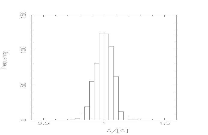
FIG. 6.: Histogram of the frequency of occurrence of samples according to their specific heat scaled by the average specific heat, for the Ising model $C_{0}$ and lattice size $l=48$ with 600 samples.

FIG. 7.: Histogram of the frequency of occurrence of samples according to their specific heat scaled by the average specific heat, for the four-state Potts model $C_{4}$ and lattice size $l=48$ with 630 samples.

2 The variance

In Fig. 8 we show the variance of $\chi$, $V_{\chi}$ of the seven critical RBAT models. For the sake of clarity (so that the data do not fall on top of each-other) $V_{\chi}$ of the model $C_{i}$ was multiplied by $2^{i+1}$. The lines are fits according to a theory which we develop in the next section. Here we just note that $V_{\chi}$ is measured with high precision, so that it may be faithfully tested against theory.

FIG. 8.: The variance of $\chi$, $V_{\chi}$ as a function of $\log l$ for all critical models, $C_{0..4}$, and $A_{2},B_{2}$ of the RBAT model. For the sake of clarity $V_{\chi}$ of the model $C_{i}$ was multiplied by $2^{i+1}$. The solid lines are fits to the form ( 51) , yielding estimates for fitting parameters which are listed in table  IV .

The relative variance $V_{\chi}/[\chi]^{2}$ is plotted in Fig. 9. Since it is the ratio of two fluctuating quantities, the errors are quite large. Nonetheless the main trends can be seen. First note that apparently for all models (except for the weakly random model $A_{2}$) $V_{\chi}/[\chi]^{2}\rightarrow\text{const}$, so that the susceptibility is non-self averaging. It is also possible that $V_{\chi}/[\chi]^{2}$ is slightly increasing with $l$ for some models ( e.g. the four state Potts model $C_{4}$ ) or slightly decreasing for the Ising model $C_{0}$. Upon comparison of the models $C_{i}\;i=0\ldots 4$ we make the following observations. The higher is the specific heat of a model, the larger is its relative variance (see Fig. 1). The higher is the exponent $(\frac{\alpha}{\nu})_{\text{pure}}$ of the pure model (see Table I), the larger is the initial slope of the relative variance of the corresponding random model. Thus the relative variance of the Ising model $C_{0}$ is the smallest and the increase with $l$, for small $l$, is the smallest. The relative variance of the four-state Potts model $C_{4}$ is the largest and the increase with $l$, for small $l$, is the largest. The relative variances of the RBAT models $C_{1,2,3}$ fall in between. The relative variance of the weakly random model $A_{2}$ shows a steady increase with $l$, in contrast with the highly random model $C_{2}$, in which a shorter increase is followed by a plateau. This is reminiscent of the specific heat of the $A_{2}$ model which exhibits very slow crossover from the power-law behavior (10) to the asymptotic logarithmic behavior (11) with a crossover length of $l_{c}\approx 50$. Thus for small lattice sizes the model $A_{2}$ exhibits effective exponents (of the specific heat) of the pure model, and also exhibits a small variance due to its small degree of randomness. But as the lattice size increases, this effect diminishes, the effective exponents approach the random value, and the variance approaches that of the highly random models.

FIG. 9.: The scaled variance of the susceptibility, $V_{\chi}/[\chi]^{2}$ as a function of $\log l$ for all critical models, $C_{0..4}$, and $A_{2},B_{2}$ of the RBAT model.

A very similar picture is obtained for the relative variance of the magnetization $V_{M}/[M]^{2}$, as seen in figure 10. The qualitative picture of the magnetization results, Fig. 10, is very similar to that of the susceptibility results, Fig. 9, showing the same trends as outlined above. Yet we emphasize that even though the magnetization is an intensive quantity, it does not seem that $V_{M}/[M]^{2}\rightarrow 0$ as $l$ increases so that the magnetization is not self averaging at criticality.

FIG. 10.: The scaled variance of $M$, $V_{M}/[M]^{2}$ as a function of $\log l$ for all critical models, $C_{0..4}$, and $A_{2},B_{2}$ of the RBAT model.

In Fig. 11 the variance of the energy $V_{E}$[27] is plotted on a log-log scale. For the sake of clarity (so that the data do not fall on top of each-other) $V_{E}$ of the model $C_{i}$ was multiplied by $2^{i+1}$ . We fit the data to the form $V_{E}\sim l^{-\theta}$ for lattice sizes $l\geq 16$ (but the fitting curves shown in Fig. 11 are not made with this form but with a more complicated one which is due to a theory which we develop in the next section). The highest value of $\theta$, $\theta=1.855(13)$, was obtained for the Ising model $C_{0}$. For the four-state Potts model, $C_{4}$, we obtained $\theta=1.72(2)$, while for the models $C_{1,2,3}$ the values of $\theta$ fell between these two values. Thus in contrast with the susceptibility and the magnetization, the variance of the energy $V_{E}$ is weakly self-averaging. But similar to the susceptibility, models with a higher specific heat or with a higher effective $\frac{\alpha}{\nu}$ have a smaller $\theta$, and thus their $V_{E}$ decreases more slowly with $l$. For the weakly random model $A_{2}$, $\theta=1.30(3)$ so that again the slope of the variance is correlated with the high slope of the specific heat of this model.

FIG. 11.: The variance of the energy, $V_{E}$ as a function of $\log l$ for all critical models, $C_{0..4}$, and $A_{2},B_{2}$ of the RBAT model. For the sake of clarity $V_{E}$ of the model $C_{i}$ was multiplied by $2^{i+1}$. The solid lines are fits to the form ( 52) , yielding estimates for the fitting parameters $a_{v},b_{v}$ which are listed in table  IV .

The results of the relative variance $V_{C}/C^{2}$, plotted in Fig. 12, seem to indicate that the specific heat is weakly self averaging. Nonetheless the effective slopes increase with $l$ (or the absolute values of the slopes decrease with $l$, this trend being strongest for the four-state Potts model $C_{4}$ ) so that it is possible that self averaging does not hold for very large $l$. It also seems possible that the Ising model is self-averaging while the other models are not. Clearly more accurate data and data from larger systems would be useful. As in other variances, we observe qualitatively that the relative variance of the moderately random models, $A_{2}$ and $B_{2}$, approaches that of the highly random ones as $l$ increases and even exceeds it.
The findings of this section are partly summarized in table III, where the self averaging properties of the highly random critical models are displayed.

FIG. 12.: The scaled variance of $C$, $V_{C}/[C]^{2}$ as a function of $\log l$ for all critical models, $C_{0..4}$, and $A_{2},B_{2}$ of the RBAT model.

TABLE III.: Summary of the self averaging properties of the critical random-bond four-state Potts $C_{4}$, Ashkin-Teller $C_{1..3}$, and Ising $C_{0}$ models. The letter ‘n’ stands for non self averaging, ‘w’ for weakly self averaging, and ‘?’ for inconclusive results. This summary is according to a subjective examination of the numerical results as displayed in figures 9 , 10 , 11 , 12 13 . According to our theory only the energy $E$ is weakly self averaging while all other quantities are non self averaging in all of these models. If the theory is correct then other behavior implied by the numerical data are merely transients.

model	$\chi$	$\chi^{(p)}$	$M$	$C$	$E$
$C_{0}$ (Ising)	?	?	?	w	w
$C_{1..3}$ (Ashkin-Teller)	n	n	n	w	w
$C_{4}$ (4 state Potts)	n	n	n	w	w

In the next section we develop a phenomenological finite size scaling theory for the variance. This theory explains the apparent connection between the variance and the specific heat behavior of the random models. In the last section we explain how this theory was applied to the results we have displayed here and discuss the comparison between our scaling theory and the numerical results.

V Finite Size Scaling of Sample to Sample Fluctuations at Criticality

As our numerical results show, we have obtained quite accurate estimates of the variance $V$ of the thermodynamic functions at the critical temperature for different lattice sizes $l$. In order to understand these results, a phenomenological theory of finite size scaling of disordered systems, which will take into account sample to sample fluctuations, needs to be developed.

The main result of our theory will be the scaling of the variance $V$ with $l$ at criticality. To be precise, we will calculate the variance $V$ of $P$ (e.g. $P=C,M,E$ or $\chi$, where all these quantities are normalized per volume; i.e. they are densities)

$$V(T,l)=[(P_{x}(T,l)-[P_{x}(T,l)])^{2}]\;.$$ (20)

$P_{x}(T,l)$ is the exact value of $P$ (that is, after the thermal fluctuations have been averaged over) of a specific sample $x$ (with some specific realization of randomly distributed bonds) of linear size $l$ at temperature $T$. Again the square brackets denote averaging over the different samples $x$.

Our conclusion will be that when the specific heat exponent $\alpha$ is negative the leading behavior of $V$ at $T_{c}$ is

$$V(T_{c},l)\sim K^{2}_{r}l^{2\rho+\frac{\alpha}{\nu}}\;,\;\;\;\;\text{ implying }\;\;\;\;\;\frac{V(T_{c},l)}{[P_{x}(T_{c},l)]^{2}}\sim l^{\frac{\alpha}{\nu}}\;.$$ (21)

Where $K_{r}$ is a measure of the amount of randomness or disorder and $\rho$ is the critical exponent of the quantity $P$, e.g. if $P=\chi$ then $\rho=\frac{\gamma}{\nu}$. Eq. (21) implies that disordered systems at criticality are only weakly self averaging when $\frac{\alpha}{\nu}<0$. For $\frac{\alpha}{\nu}=0_{+}$ (log), as was found[11] for the random bond Ashkin-Teller model, our derivation is strictly not valid for $l\gg 1$. Nonetheless for the range of lattice sizes considered, we found good agreement between the numerical results for the variance of $\chi,\chi_{p}$ and $E$ and theoretical fits according to (21) together with next to leading terms (see figures 8 , 13 and 11 and discussion in the next section). If no dramatic change occurs at larger sizes, then the sample to sample fluctuations of the random bond Ashkin-Teller model are non self averaging.

The result (21) indicates that the sample to sample fluctuations at the critical temperature $T_{c}$ depend strongly on the specific heat exponent $\frac{\alpha}{\nu}$. This strong dependence can be made plausible based on heuristic arguments. These heuristic arguments will serve to define some basic ingredients of our approach and will be followed by a more quantitative treatment.

We start by characterizing every specific sample $x$ of size $l$ by a pseudo-critical temperature $T_{c}(x,l)$. This pseudo-critical temperature can, for instance, be the temperature at which a maximum in the specific heat of the sample occurs. We denote the average pseudo-critical temperature as $T_{c}(l)=[T_{c}(x,l)]$. We assume that, as is the case in homogeneous systems,

$$T_{c}(l)-T_{c}=al^{-y_{t}}\;,$$ (22)

where $a$ is a constant, $y_{t}=1/\nu$ and $T_{c}=\lim_{l\rightarrow\infty}T_{c}(l)$. $T_{c}$ is the average critical temperature of the ensemble of infinite samples. Eq. (22) is supported by a numerical study[28] of the three dimensional dilute Ising model.

Next we assume that $T_{c}(x,l)$ fluctuates around $T_{c}(l)$ with width

$$\delta T_{c}(l)\sim l^{-d/2}\;.$$ (23)

This assumption is probably true[1, 12] for small disorder and small $l$, or close to the pure system fixed point. We assume it without proof, for large disorder as well, though for large disorder (or close to the random fixed point) the possibility that $\delta T_{c}(l)\sim l^{-y_{t}}$ has been raised[29].
Define reduced temperatures

$$t_{c}(x,l)=\frac{T_{c}(x,l)-T_{c}}{T_{c}}\;,$$ (25)

$$t_{c}(l)=\frac{T_{c}(l)-T_{c}}{T_{c}}\;,$$ (26)

and the reduced width

$$\delta t_{c}(l)=\frac{\delta T_{c}(l)}{T_{c}}\;.$$ (27)

We make (23) more specific by assuming for $t_{c}(x,l)$ a Gaussian probability distribution $q(t_{c}(x,l))$

$$q(t_{c}(x,l))=\frac{l^{d/2}}{\sqrt{2\pi}K_{r}}\exp\{-[t_{c}(x,l)-t_{c}(l)]^{2}l^{d}/2K^{2}_{r}\}\;.$$ (28)

The width of the distribution is controlled by the lattice size $l$ and by $K_{r}$ which is a measure of the amount of randomness or disorder.

The scaling relations (22, 23) already make the result (21) plausible. The main idea is that the sample to sample fluctuations at $T_{c}$ are governed by the relative magnitude of two temperature differences. The first is the difference between the average pseudo-critical temperature $T_{c}(l)$ and the critical temperature of the infinite system $T_{c}$. The second is the difference between $T_{c}(l)$ and $T_{c}(x,l)$, the pseudo-critical temperature of the sample $x$, which is governed by $\delta t_{c}(l)$. If $\delta t_{c}(l)\gg|t_{c}(l)|$ then fluctuations in $t_{c}(x,l)$ are so large that for some samples one will find $T_{c}>T_{c}(x,l)$ while for other samples $T_{c}<T_{c}(x,l)$. In this case, even though we are simulating all samples at $T_{c}$, some samples are in their high temperature phase while others are in their low temperature phase. This will obviously increase the sample to sample fluctuations in any observable. If, on the other hand, $\delta t_{c}(l)\ll|t_{c}(l)|$, then $T_{c}-T_{c}(x,l)$ will always have the same sign and fluctuations will be smaller. The condition $\delta t_{c}(l)\ll|t_{c}(l)|$ will be fulfilled for large $l$ if $y_{t}-\frac{d}{2}<0$ or, using the hyper-scaling relation $\frac{\alpha}{\nu}=2y_{t}-d$, if $\frac{\alpha}{\nu}<0$. For disordered systems, the bound $y_{t}\leq d/2$ has been proven by Chayes et al.[30], so that asymptotically one always finds $\frac{\alpha}{\nu}\leq 0$. However, for small $l$ and small disorder, the system may be governed by a positive $(\frac{\alpha}{\nu})_{\text{pure}}$. In this case sample to sample fluctuations can increase with lattice size, as is indeed seen in our numerical results for the weakly disordered model $A_{2}$. Thus on the basis of these considerations one can conclude that the sign and magnitude of the specific heat exponent $\alpha$ of the disordered model have a strong influence on the sample to sample fluctuations [26], and will determine whether they are self averaging. The discussion above is analogous to the physical arguments leading to the Harris criterion[12], but in a finite size scaling formulation. The difference is that the Harris criterion was derived near the pure system fixed point, while we are assuming that similar conditions apply also next to the disordered critical fixed point.

In order to put these general considerations on more quantitative grounds, we proceed to derive the finite-size scaling expression (21) for the variance of various thermodynamic quantities. Start by introducing the reduced temperature of each sample $x$;

$$\dot{t}_{x}=\frac{T-T_{c}(x,l)}{T_{c}}\;.$$ (29)

We assume ( for samples with $T$ close to $T_{c}(x,l)$) a finite size scaling form for the singular part of $P_{x}$,

$$P^{\text{sing}}_{x}(T,l)=l^{\rho}\tilde{Q}_{x}(\dot{t}_{x}l^{y_{t}})\;.$$ (30)

The form of the function $\tilde{Q}_{x}(Z)$ (or its coefficients) are assumed to be sample dependent but the critical exponents $\rho,y_{t}$ are assumed to be universal or sample independent.

eq. (30) embodies the usual[31] finite size scaling assumption that in the vicinity of the critical temperature the behaviour of a large finite system is governed by the scaled variable $\xi_{x}/l$. We use this assumption, even though in the present context it implies that a single correlation length $\xi_{x}$ is sufficient to describe the state of a disordered sample, which is not obvious at all. This “thermal” $l$ -dependence is compounded by the fact that if we increase $l$, we must generate additional random bonds, and hence increasing $l$ necessitates, effectively, changing $x$ (that represents a particular realization of the random bond variables). Since $x$ affects $P^{sing}_{x}$ through the non-universal coefficients of $\tilde{Q}_{x}$, a non-thermal dependence of $P^{sing}_{x}$ on $l$ is induced. The main task of our analysis is to separate the thermal $l$ dependence from the non-thermal component.

At this stage it is possible to draw some more conclusions based on (30), without making strong assumptions about the coefficients of $\tilde{Q}_{x}$. We leave such derivations for the Appendix. Here we proceed in a more straightforward manner by using a simplifying ansatz. Our ansatz states that the coefficients of $\tilde{Q}_{x}$ depend only on $\Delta t_{c}(x,l)$, the deviation of the pseudo-critical temperature of the sample from the average pseudo-critical temperature, defined as

$$\Delta t_{c}(x,l)=t_{c}(x,l)-t_{c}(l)\;.$$ (31)

It is convenient to proceed by rewriting $\dot{t}_{x}$ as $\dot{t}_{x}=t-\Delta t_{c}(x,l)-t_{c}(l)$ with $t=\frac{T-T_{c}}{T_{c}}$. Using the scaling of $t_{c}(l)$ [see (22) and (26)] , we substitute $\tilde{Q}_{x}$ by a different scaling function $Q_{x}$ and rewrite Eq. (30) as

$$P^{sing}_{x}(T,l)=l^{\rho}\tilde{Q}_{x}\{(t-\Delta t_{c}(x,l)-t_{c}(l))l^{y_{t}}\}=l^{\rho}Q_{x}\{(t-\Delta t_{c}(x,l))l^{y_{t}}\}\;.$$ (32)

For completeness of the treatment which will later prove to be necessary we do not neglect the analytic dependence of $P_{x}(T,l)$ on $(t-\Delta t_{c}(x,l))$[32], and write

$$P_{x}(T,l)=A_{x}+B_{x}(t-\Delta t_{c}(x,l))+C_{x}(t-\Delta t_{c}(x,l))^{2}+\ldots+l^{\rho}Q_{x}\{(t-\Delta t_{c}(x,l))l^{y_{t}}\}\;.$$ (33)

The coefficients $A_{x},B_{x},C_{x}$ are assumed to be sample dependent in the same way that the coefficients of $Q_{x}$ are; namely they depend only on $\Delta t_{c}(x,l)$[33]. Next, assume the dependence of the coefficients on $\Delta t_{c}(x,l)$ is analytic. Since according to (28) and (31), $\Delta t_{c}(x,l)$ is distributed around zero with width that scales as $l^{-d/2}$, we can expand

$$A_{x}=A_{0}+A_{1}\Delta t_{c}(x,l)+A_{2}(\Delta t_{c}(x,l))^{2}+\ldots\;,$$ (34)

where $A_{0},A_{1},A_{2}$ are sample independent. The same type of expansion is assumed for $B_{x},C_{x}$ etc.

We are interested in knowing what happens at $T=T_{c}$, the average critical temperature of the ensemble of infinite samples. Thus we set $T=T_{c}$ which implies $t=0$. For the analytic part of (33) we get

$$P_{x}^{\text{analytic}}(T_{c},l)= A_{x}-B_{x}\Delta t_{c}(x,l)+C_{x}\Delta t_{c}(x,l)^{2}+\ldots=$$ (35)

$$A_{0}+(A_{1}-B_{0})\Delta t_{c}(x,l)+(A_{2}-B_{1}+C_{0})(\Delta t_{c}(x,l))^{2}+\ldots$$ (36)

$$\equiv a+b\Delta t_{c}(x,l)+c(\Delta t_{c}(x,l))^{2}\;,$$ (37)

where the second equality is reached by use of (34) and the same expansions for other coefficients. The last equality is a redefinition of constants. In a similar way we expand $Q_{x}$

$$Q_{x}(Z)=D_{x}+E_{x}Z+F_{x}Z^{2}+\ldots\;,$$ (38)

where $D_{x},E_{x},F_{x}$ are again expanded as in (34). Again setting $t=0$, we obtain for the singular part of (33)

$$P_{x}^{singular}(T_{c},l)=l^{\rho}\{D_{0}+(D_{1}-E_{0}l^{y_{t}})\Delta t_{c}(x,l)+(D_{2}-E_{1}l^{y_{t}}+F_{0}l^{2y_{t}})(\Delta t_{c}(x,l))^{2}\}+\ldots\;.$$ (39)

We stress that since we set $Z=-\Delta t_{c}(x,l)l^{y_{t}}$, $Z$ is fluctuating around zero with width that scales as $\sim l^{\frac{\alpha}{2\nu}}$. Thus the expansion (38) is justified asymptotically only for $\alpha<0$. Putting together (37) and (39) we have

$$P_{x}(T_{c},l)= (a+D_{0}l^{\rho})+(b+D_{1}l^{\rho}-E_{0}l^{\rho+y_{t}})\Delta t_{c}(x,l)+$$ (40)

$$(c+D_{2}l^{\rho}-E_{1}l^{\rho+y_{t}}+F_{0}l^{\rho+2y_{t}})(\Delta t_{c}(x,l))^{2}+\ldots\equiv d+e\Delta t_{c}(x,l)+f(\Delta t_{c}(x,l))^{2}\;.$$ (41)

Notice that here the only dependence on the specific sample $x$ is through explicit dependence on $\Delta t_{c}(x,l)$, the deviation of its reduced pseudo-critical temperature from the average pseudo-critical temperature. Taking the quenched sample average [ ] with the probability distribution (28), using $[\Delta t_{c}(x,l)]=0$, we get

$$[P_{x}(T_{c},l)]=d+f[(\Delta t_{c}(x,l))^{2}]\;,$$ (42)

and using $[(\Delta t_{c}(x,l))^{3}]=0$ we further obtain

$$[(P_{x}(T_{c},l))^{2}]=d^{2}+e^{2}[(\Delta t_{c}(x,l))^{2}]+f^{2}[(\Delta t_{c}(x,l))^{4}]+2df[(\Delta t_{c}(x,l))^{2}]\;.$$ (43)

The variance is then given by

$$V(T_{c},l)=e^{2}[(\Delta t_{c}(x,l))^{2}]+f^{2}\{[(\Delta t_{c}(x,l))^{4}]-[(\Delta t_{c}(x,l))^{2}]^{2}\}=e^{2}[(\Delta t_{c}(x,l))^{2}]+2f^{2}[(\Delta t_{c}(x,l))^{2}]^{2}\;,$$ (44)

where the last equality is a property of the Gaussian distribution. Lastly we use $[(\Delta t_{c}(x,l))^{2}]=K^{2}_{r}l^{-d}$ and obtain to the leading orders in $l$

$$V(T_{c},l)= (b^{2}+D_{1}^{2}l^{2\rho}+E_{0}^{2}l^{2\rho+2y_{t}}+2bD_{1}l^{\rho}-2bE_{0}l^{\rho+y_{t}}-2D_{1}E_{0}l^{2\rho+y_{t}})K^{2}_{r}l^{-d}+$$ (45)

$$(F_{0}^{2}l^{2\rho+4y_{t}})2K^{4}_{r}l^{-2d}+\ldots\;.$$ (46)

Since $y_{t}>0$, and usually $\rho+y_{t}>0$, the leading term in (46) is

$$V(T_{c},l)\sim E_{0}^{2}K^{2}_{r}l^{2\rho+2y_{t}-d}=E_{0}^{2}K^{2}_{r}l^{2\rho+\frac{\alpha}{\nu}}\;.$$ (47)

The last term in (46) is proportional to $K^{4}_{r}l^{2\rho+2\frac{\alpha}{\nu}}$, and may be neglected with respect to (47) only for $\frac{\alpha}{\nu}<0$, or if $K^{2}_{r}\ll 1$ and $l$ is not too large. (47) is our main result for the variance, where all exponents $\rho,\alpha,\nu$ are exponents that characterize the disordered system. It means that disordered systems at criticality are only weakly self averaging when $\frac{\alpha}{\nu}<0$. Though our derivation is not valid when $\frac{\alpha}{\nu}=0_{+}$ ($C\sim\log l$) it seems that in this case there is no self averaging of the sample to sample fluctuations.This point is further discussed in the next section.

We note that for $\alpha<0$ and in the large $l$ limit considered at the end of the Appendix [equation (60) ], where

$$Q_{x}(-\Delta t_{c}(x,l)l^{y_{t}})\rightarrow Q(-\Delta t_{c}(x,l)l^{y_{t}})\;,$$ (48)

the coefficients of $Q_{x}$ are independent of $x$ so that $D_{x}=D_{0},E_{x}=E_{0}$ etc. . Neglecting the analytic part of $P$, this limit corresponds to our derivation with only $D_{0},E_{0},F_{0}\not=0$ and all other coefficients ( $D_{1},D_{2},E_{1}$ etc. ) equal to zero. Thus in this limit the main result (47) is unchanged, though less assumptions are needed.

From (42) corrections to the scaling of $P$ are obtained,

$$[P_{x}(T_{c},l)]=a+D_{0}l^{\rho}+(c+D_{2}l^{\rho}-E_{1}l^{\rho+y_{t}}+F_{0}l^{\rho+2y_{t}})K^{2}_{r}l^{-d}\;.$$ (49)

So that the leading behaviour of $P$ is

$$[P_{x}(T_{c},l)]=a+D_{0}l^{\rho}+F_{0}K^{2}_{r}l^{\rho+2y_{t}-d}=a+D_{0}l^{\rho}+F_{0}K^{2}_{r}l^{\rho+\frac{\alpha}{\nu}}\;.$$ (50)

Thus for negative $\alpha$, the third term in (50) is a correction to scaling due to sample to sample fluctuations. It follows that for $\frac{\alpha}{\nu}<0$, (50) and (47) are consistent with $V/[P]^{2}\sim l^{\frac{\alpha}{\nu}}$. A special case is when $\alpha_{\text{pure}}<0$ and randomness is an irrelevant operator (at the pure system fixed point) with a scaling exponent $(\frac{\alpha}{\nu})_{\text{pure}}$. In this case the disordered system has the same exponents as the pure one, $\frac{\alpha}{\nu}=(\frac{\alpha}{\nu})_{\text{pure}}$. Therefore the correction to scaling we have obtained due to sample to sample fluctuations has the same exponent as the correction term connected with the irrelevant operator corresponding to randomness.

VI Comparison of Theory with Variance Results of the RBAT models

The derivation presented in the previous section as can be readily seen from equations (33, 34, 38), involved an expansion in the two parameters $\sqrt{[(\Delta t_{c}(x,l))^{2}]}$ and $\sqrt{[(\Delta t_{c}(x,l))^{2}]}l^{y_{t}}$. These scale as $K_{r}l^{-\frac{d}{2}}$ and $K_{r}l^{y_{t}-\frac{d}{2}}=K_{r}l^{\frac{\alpha}{2\nu}}$. Thus the derivation is valid for small $K_{r}$, meaning small disorder and small $\frac{\alpha}{\nu}$. For negative $\frac{\alpha}{\nu}$ the validity of the expansion improves as $l$ increases, while a positive $\frac{\alpha}{\nu}$ is not possible[30].

In the case of the random bond Ashkin Teller model, we have asymptotically $C\approx b\log l$ so that $\frac{\alpha}{\nu}=0_{+}$. It seems that in this case the expansion is not justified. Practically though, for the accessible range of lattice sizes, things depend on the constant of proportionality $b$. If $b$ is small, then for a finite but large interval of lattice sizes $l$ the expansion is justified. Indeed, in the case of the highly random RBAT models $C_{0\ldots 4}$, $b$ falls in the range $0.138(4)\leq b\leq 0.280(6)$. Upon inspection of Fig. 1 one may also see that the value of the specific heat of these models shows very little variation for lattice sizes $l\geq 16$. Thus the parameter $K_{r}l^{\frac{\alpha}{\nu}}$, which should scale with $l$ as the specific heat does, increases very slowly with $l$. This implies that for the accessible range of lattice sizes $l$ our expansion is valid. The specific heat of the weakly random model $A_{2}$ effectively diverges with a positive effective $\frac{\alpha}{\nu}$ but because of its weak degree of randomness there is good reason to believe that the expansion will be valid due to a small value of $K_{r}$ expected for models with small randomness. The $B_{2}$ model with moderate disorder is expected to fall between the $A_{2}$ model and the $C_{0\ldots 4}$ models. Thus there is reason to hope that our theory is applicable to the variance results in the accessible range $4\leq l\leq 256$. Indeed the agreement we now display between numerical data and theory is good.

For observables with $\rho>0$ the two leading terms in (46) are the third and sixth terms. We use hyper-scaling to write $l^{y_{t}}=l^{\frac{\alpha}{2\nu}+\frac{d}{2}}$ and substitute in (21) $l^{\frac{\alpha}{\nu}}$ by the behaviour of the specific heat (8). Thus we propose for the RBAT models the leading behaviour[34]

$$V(T_{c},l)=a_{v}l^{2\rho}\ln[1+c_{0}(l^{(\alpha/\nu)_{\text{pure}}}-1)]+c_{v}l^{2\rho-\frac{d}{2}}\{\ln[1+c_{0}(l^{(\alpha/\nu)_{\text{pure}}}-1)]\}^{\frac{1}{2}}\;,$$ (51)

with $a_{v}\equiv E_{0}^{2}K_{r}^{2}$ and $c_{v}\equiv-2D_{1}E_{0}K_{r}^{2}$ (note that for every thermodynamic quantity there are different coefficients $E_{0},D_{1}$ etc. ) The expression $\ln[1+c_{0}(l^{(\alpha/\nu)_{\text{pure}}}-1)]$ describes the singular behavior of the specific heat including the crossover from the pure model behavior , characterized by the pure model exponent $(\alpha/\nu)_{\text{pure}}$ (see Eq. (8) ). $\rho$ is the critical exponent of the quantity whose variance is measured (e.g. $\rho=\frac{\gamma}{\nu}$ for $\chi$ and $\rho=\frac{\gamma^{(p)}}{\nu}$ for $\chi^{(p)}$ ).

In fig. 8 we show the variance of $\chi$, $V_{\chi}$ of the seven critical RBAT models fitted by the function (51), where the parameters $c_{0},(\alpha/\nu)_{\text{pure}}$ and $\frac{\gamma}{\nu}$ were taken from Tables I and II. For the sake of clarity (so that the data do not fall on top of each-other) $V_{\chi}$ of the model $C_{i}$ was multiplied by $2^{i+1}$. The fitting parameters $a_{v},c_{v}$ are given in Table IV. The agreement with our scaling prediction is quite encouraging. TABLE IV.: Fitting parameters for the variances of $\chi,\chi^{(p)},E$ for the critical models $C_{0..4}$, and $A_{2},B_{2}$ according to eq-s.  (51 ) and (52 ), using lattice sizes $l\geq 8$. $V_{\chi}$ $V_{\chi^{(p)}}$ $V_{E}$ $a_{v}$ $c_{v}$ $a_{v}$ $c_{v}$ $a_{v}$ $b_{v}$ $C_{0}$(Ising) 0.0145(7) 0.11(2) 0.033(1) .07(4) 0.29(7) 0.8(2) $C_{1}$ 0.0039(1) 0.026(10) 0.0134(3) -0.03(2) 0.128(14) -1.45(19) $C_{2}$ 0.0059(1) 0.014(10) 0.0172(2) -0.09(2) 0.135(13) -1.19(16) $C_{3}$ 0.0069(2) -0.01(1) 0.0147(3) -0.12(2) 0.133(15) -1.27(18) $C_{4}$(Potts) 0.0082(2) -0.04(1) 0.082(2) -0.04(1) 0.121(13) -1.25(17) $B_{2}$ 0.033(1) 0.13(2) 0.092(2) 0.19(4) 0.99(15) 1.2(2) $A_{2}$ 0.056(1) 0.028(12) 0.143(3) 0.05(3) 5.49(44) 1.28(23) The same analysis has been carried out for the variance of $\chi^{(p)}$, where $\frac{\gamma^{(p)}}{\nu}$ was taken from Table II, and the results are plotted in fig. 13. Again the fitting parameters $a_{v},c_{v}$ are given in Table IV and the agreement between the numerical results and our scaling prediction is encouraging. We stress that the only fitting parameters of the fits in figures 8 and 13 are $a_{v}$ $c_{v}$; the other parameters of eq. (51), $\rho,c_{0},(\alpha/\nu)_{p}$ were obtained previously[11] from the specific heat results and from the results for $\chi$ and $\chi^{(p)}$.

FIG. 13.: The variance of $\chi^{(p)}$, $V_{\chi^{(p)}}$ as a function of $\log l$ for all critical models, $C_{0..4}$, and $A_{2},B_{2}$ of the RBAT model. For the sake of clarity $V_{\chi^{(p)}}$ of the model $C_{i}$ was multiplied by $2^{i+1}$. The solid lines are fits to the form ( 51) , yielding estimates for fitting parameters which are listed in table  IV .

Since the first term in (51) is the dominant one (by a factor of $l^{y_{t}}$, where $y_{t}\geq 1$ ), we test (51) again in another manner. in fig. 14 we plot the scaled $V_{\chi}$ : $V_{\chi}l^{-2\rho}/\ln[1+c_{0}(l^{(\alpha/\nu)_{\text{pure}}}-1)]$. Indeed it seems that the data points approach a constant value, confirming the leading term in (51) which originates in the leading behavior of the variance (47).

FIG. 14.: The scaled variance of $\chi$, $V_{\chi}l^{-2\frac{\gamma}{\nu}}/\ln[1+c_{0}(l^{(\alpha/\nu)_{\text{p}}}-1)]$ as a function of $\log l$ for all critical models, $C_{0..4}$, and $A_{2},B_{2}$ of the RBAT model.

For the energy $\rho=(\alpha-1)/\nu<0$ so that the two leading terms in (46) are the third and the fifth ones. Again by using hyper-scaling and substituting $l^{\frac{\alpha}{\nu}}$ by the behaviour of the specific heat (8), we arrive at the scaling form for the variance of the energy

$$V_{E}(T_{c},l)=\{a_{v}(\ln[1+c_{0}(l^{(\alpha/\nu)_{\text{pure}}}-1)])^{2}+b_{v}\ln[1+c_{0}(l^{(\alpha/\nu)_{\text{pure}}}-1)]\}l^{-d}\;,$$ (52)

with $b_{v}=-2bE_{0}K_{r}^{2}$ In fig. 11 we show the variance of the energy, $V_{E}$ of the seven critical RBAT models fitted by the function (52). For the sake of clarity $V_{E}$ of the model $C_{i}$ was multiplied by $2^{i+1}$. The agreement between theory and the numerical data is good and the fitting parameters $a_{v},b_{v}$ are given in table IV.

For the magnetization and the specific heat $\rho=\frac{\alpha}{\nu}$ and $\rho=\frac{-\beta}{\nu}$ respectively. In these cases $|\rho|$ is small and the fifth and the sixth terms in Eq. (46) are of similar order in $l$ . Thus one may not neglect one term with respect to the other as was done for the energy and the susceptibility. Thus we fit the variance of the specific heat to the form

$$V_{C}(T_{c},l)=a_{v}\{\ln[1+c_{0}(l^{(\alpha/\nu)_{\text{pure}}}-1)]\}^{3}+b_{v}l^{-\frac{d}{2}}\{\ln[1+c_{0}(l^{(\alpha/\nu)_{\text{pure}}}-1)]\}^{1.5}+$$ (53)

$$c_{v}l^{-\frac{d}{2}}\{\ln[1+c_{0}(l^{(\alpha/\nu)_{\text{pure}}}-1)]\}^{2.5}\;.$$ (54)

In fig. 15 the variance of the specific heat, $V_{C}$ of the seven critical RBAT models is fitted by the function (54), with the fitting coefficients given in Table V. TABLE V.: Fitting parameters for the variances of the specific heat $V_{C}$ and the magnetization $V_{M}$ for the critical models $C_{0..4}$, and $A_{2},B_{2}$ according to eq-s.  (54 ) and (56 ), using lattice sizes $l\geq 4$. $V_{C}$ $V_{M}$ $a_{v}$ $b_{v}$ $c_{v}$ $a_{v}$ $b_{v}$ $c_{v}$ $C_{0}$(Ising) 0.000016(12) 0.028(10) 0.008(4) 0.0037(1) 0.25(2) -0.28(2) $C_{1}$ 0.0000011(1) -0.045(4) 0.0038(3) 0.00108(3) 0.102(9) -0.12(1) $C_{2}$ 0.0000028(5) -0.078(8) 0.0081(7) 0.00169(7) 0.10(2) -0.12(2) $C_{3}$ 0.0000079(6) -0.069(5) 0.0069(5) 0.00213(9) 0.054(20) -0.068(24) $C_{4}$(Potts) 0.0000099(4) -0.062(5) 0.0057(4) 0.0027(1) -0.004(23) -0.004(28) $B_{2}$ 0.0079(6) -0.44(9) 1.4(1) 0.0089(3) 0.27(3) -0.30(4) $A_{2}$ 0.67(7) -4.9(18) 36.5(54) 0.0167(8) 0.07(7) -0.07(10) The data for large lattice sizes is rather noisy and three parameter fits are not so reliable with only eleven data points, so that both the results and the fitting curves in Fig. 15 should be taken with a grain of salt. The obtained fitting coefficients are consistent with the coefficient $E_{0}$ being much smaller than $b,D_{1}$. A small value for $E_{0}$ is quite plausible if the specific heat as a function of the temperature is close to being symmetric around the critical point [see (38)]. This symmetry is supported by the symmetric form of the histograms of the specific heat as shown in figures 6 and 7. For the Ising model $C_{0}$ the errors of the coefficients $a_{v},b_{v}$ and $c_{v}$ are of the same order of magnitude as the coefficients themselves. However for the other models the errors are reasonable and though $a_{v}$ is small, we have $E_{0}^{2}K_{r}^{2}\equiv a_{v}>0$, meaning that, asymptotically, the first term in (54) will dominate. This implies that the specific heat of the RBAT models is non self averaging, excluding possibly the random bond Ising model. possibly, the theory needs some changes in order to be applied to the specific heat $C$ which diverges logarithmically (and as a double logarithm for the random bond Ising model) and not with a simple power law.

FIG. 15.: The variance of the specific heat, $V_{C}$ as a function of $\log l$ for all critical models, $C_{0..4}$, and $A_{2},B_{2}$ of the RBAT model. The solid lines are fits to the form ( 54) , yielding estimates for the fitting parameters $a_{v},b_{v},c_{v}$ which are listed in table  V .

In fig. 16 the variance of the magnetization, $V_{M}$ of the seven critical RBAT models is fitted by the function

$$V_{M}=a_{v}l^{-2\frac{\beta}{\nu}}\ln[1+c_{0}(l^{(\alpha/\nu)_{\text{pure}}}-1)]+b_{v}l^{-\frac{\beta}{\nu}-\frac{d}{2}}\{\ln[1+c_{0}(l^{(\alpha/\nu)_{\text{pure}}}-1)]\}^{\frac{1}{2}}+$$ (55)

$$c_{v}l^{-2\frac{\beta}{\nu}-\frac{d}{2}}\{\ln[1+c_{0}(l^{(\alpha/\nu)_{\text{pure}}}-1)]\}^{\frac{1}{2}}\;.$$ (56)

The fitting coefficients $a_{v},b_{v}$ and $c_{v}$ are given in Table V. The data are much more noisy than the data of the susceptibility (see Fig. 8).

FIG. 16.: The variance of the magnetization, $V_{M}$ as a function of $\log l$ for all critical models, $C_{0..4}$, and $A_{2},B_{2}$ of the RBAT model. The solid lines are fits to the form ( 56) , yielding estimates for the fitting parameters $a_{v},b_{v},c_{v}$ which are listed in table  V .

To summarize, we have examined the sample to sample fluctuations in various thermodynamic quantities of some random bond Ashkin Teller models. These include the random bond Ising and four state Potts models. It was found that far from criticality all thermodynamic quantities examined are strongly self averaging (that is their variance scales as $l^{-d}$) . At the critical point we found that the susceptibility $\chi$, the susceptibility of the polarization $\chi^{(p)}$ and the magnetization $M$ are non self averaging, while the energy $E$ is weakly self averaging. The data for the variance of the specific heat seems to imply weak self averaging of the specific heat. Since the data are not accurate at the larger sizes used, this may well be a transient behavior, compatible with our theory which predicts that asymptotically the specific heat is non self averaging. A phenomenological finite size scaling theory was developed for the sample to sample fluctuations. Its main prediction is that when the specific heat exponent $\alpha<0$ ($\alpha$ of the disordered model) then, for a quantity $P$ which scales as $l^{\rho}$ at criticality, its variance $V_{P}$ will scale asymptotically as $l^{2\rho+\frac{\alpha}{\nu}}$. The theory is not applicable in the asymptotic limit ($l\rightarrow\infty$) to cases where $\frac{\alpha}{\nu}=0_{+}$. Nonetheless in the accessible range of lattice sizes we found very good agreement between the theory and the data for $V_{\chi},V_{\chi^{(p)}}$ and $V_{E}$. The data for $V_{\chi}$ is especially convincing. The theory also describes well the variance of models with weak disorder, exhibiting slow crossover to the randomness dominated behavior. The theory may also be compatible with the data for $V_{M}$ and $V_{C}$, but evidence for this is less convincing. We note that if our assumption (23) is incorrect and should be replaced asymptotically by[29] $\delta T_{c}(l)\sim l^{-y_{t}}$, then our theory predicts that $V_{P}\sim l^{2\rho}$ independent of $\alpha$. In this case all quantities (excluding the energy which has a non vanishing non singular part) are non self averaging independent of $\alpha$.
In order to further test our theory we intend to study the sample to sample fluctuations in the site dilute three dimensional Ising model where $\frac{\alpha}{\nu}<0$ and our analysis holds.

In this section we draw some more conclusions based on the finite size scaling form (30), without making any assumptions on the explicit $x$ dependence of the coefficients of $\tilde{Q}_{x}$.

What can we deduce about the coefficients of $\tilde{Q}_{x}$ from the Brout argument? Consider (30) in the limit $l\rightarrow\infty$, $\dot{t}_{x}$ finite. In this case $\xi$ is finite, the Brout argument holds, and one expects $P_{x}(T)$ to be sample independent. This means that in this limit we expect the coefficients of $\tilde{Q}_{x}$ and its argument to converge to some $x$ independent values. It follows that we can assume that these coefficients are distributed according to some unknown distribution function whose width $w(l)$ depends on $l$ and tends to zero as $l\rightarrow\infty$.

Is there any limit in which one may recover the usual finite size scaling behaviour, completely independent of the specific sample $x$? Consider the limit $l$ large but finite and $T\approx T_{c}$. Let us now add the assumption that the width $w(l)$ tends to zero no slower than $l^{-d/2}$ . Then for large enough $l$, according to equations (23-29), $\dot{t}_{x}$ approaches $\dot{t}$ given by

$$\dot{t}=\frac{T-T_{c}(l)}{T_{c}}$$ (57)

as $l^{-d/2}$, and

$$\tilde{Q}_{x}(\dot{t}_{x}l^{y_{t}})\rightarrow\tilde{Q}(\dot{t}l^{y_{t}})\;,$$ (58)

so that we recover the usual[31] finite size scaling behaviour.

The limit (58) cannot account for the large sample to sample fluctuations that we have numerically observed at $T=T_{c}$ even for rather large values of $l$. Indeed, special care is needed in the case $T=T_{c}$, where $\xi/l$ is not small and the Brout argument does not hold. It turns out that in this case the limit, where the $x$ dependence of $\dot{t}_{x}$ can be ignored as in (58), does not occur or is reached ‘slowly’. When $T=T_{c}$, then $\dot{t}_{x}=-t_{c}(x,l)=\{t_{c}(l)-t_{c}(x,l)\}-t_{c}(l)$, so that according to (23) and (22) $\dot{t}_{x}$ is a difference of a fluctuating term of order $l^{-d/2}$ and a term of a constant sign of order $l^{-y_{t}}$. Therefore

$$\frac{|\delta\dot{t}_{x}|}{|\dot{t}_{x}|}\sim\left\{\begin{array}[]{ll}\,l^{y_{t}-d/2}=l^{\frac{\alpha}{2\nu}}=l^{-|\frac{\alpha}{2\nu}|}&\mbox{if }\;\;d/2>y_{t}\;\;\;(\alpha<0)\\ \,1&\mbox{if }\;\;d/2\leq y_{t}\;\;\;(\alpha\geq 0)\end{array}\right.\;.$$ (59)

Thus for $T=T_{c}$ and positive $\alpha$,  $\dot{t}_{x}\not\rightarrow\dot{t}$ for large $l$ and (58) is not justified. In this case the relative fluctuations in the argument of $\tilde{Q}_{x}$ are of order 1 and their absolute magnitude scales as $l^{\frac{\alpha}{2\nu}}$ so that it increases with $l$. So for large $l$ the argument of $\tilde{Q}_{x}$ is a constant plus a large fluctuating quantity which increases with $l$. It follows that $\tilde{Q}_{x}$ cannot be expanded as is done in Sec. V, and that the limit (58) does not exist.

For negative $\alpha$ it follows that the fluctuations in the argument of $\tilde{Q}_{x}$ scale as $l^{-|\frac{\alpha}{2\nu}|}$. Since we have assumed that the fluctuations in the coefficients of $\tilde{Q}_{x}$, $w(l)$, scale as $l^{-d/2}$ then if $|\frac{\alpha}{2\nu}|<\frac{d}{2}$ then at $T=T_{c}$  $w(l)$ decreases faster than the fluctuations in the argument of $\tilde{Q}_{x}$. Thus one may consider the range of $l$ for which

$$\tilde{Q}_{x}(\dot{t}_{x}l^{y_{t}})\rightarrow\tilde{Q}(\dot{t}_{x}l^{y_{t}})\;,$$ (60)

where only the argument of $\tilde{Q}_{x}$ is $x$ dependent. In this case the coefficients of $\tilde{Q}$ are some constants for which we need not assume anything about their $x$ or $l$ dependence. Consideration of the limit (60) suffices to reach our main result (21) (but not corrections to (21)), independent of the assumptions made in Sec. V on the $x$ dependence of the coefficients of $\tilde{Q}_{x}$.

REFERENCES

- [1] R.B. Stinchcombe , in Phase Transitions and Critical Phenomena,edited by C. Domb and J.L. Lebowitz(Academic, New York, 1983), vol. 7.
- [2] B.N. Shalaev, Physics reports237, 129 (1994).
- [3] W. Selke, L.N. Schur and A.L. Talapov, in ”Annual Reviews of Computational Physics”, ed. D. Stauffer, World Scientific, Singapore p. 17 (1994).
- [4] It is probably more accurate to refer to an average correlation length.
- [5] M.N. Barber, in Phase Transitions and Critical Phenomena, edited by C. Domb and J.L. Lebowitz, vol. 8.
- [6] K. Binder and A.P. Young, Rev. Mod. Phys.58, 837 (1986) and references therein.
- [7] R. Brout, Phys. Rev.115, 824 (1959).
- [8] A.B. Harris, S. Kim and T.C. Lubensky, Phys. Rev. Lett.53, 743 (1984); 54, 1088(E) (1985); R. Rammal, M.A. Lemieux and A.-M.S. Tremblay, Phys. Rev. Lett.54, 1087(C) (1985); A.B. Harris, Y. Meir and A. Aharony Phys. Rev. B41, 4610 (1990) and references therein.
- [9] K. Binder, D.W. Heermann, Monte Carlo Simulations in Statistical Physics. Springer-Verlag, Berlin, (1988).
- [10] A. Milchev, K. Binder, and D.W. Heermann, Z. Phys. B - Condensed Matter 63, 521 (1986).
- [11] S. Wiseman and E. Domany, Phys. Rev E 51, 3074.
- [12] A.B. Harris J.Phys. C,7:1671,(1974).
- [13] J. Ashkin and E. Teller, Phys. Rev.64, 178 (1943).
- [14] R. Fisch J. Stat. Phys.,18:111,(1978).
- [15] W.Kinzel and E. Domany Phys. Rev. B,23:3421, (1981).
- [16] F.Y. Wu and K.Y. Lin, J.Phys. C7, L181 (1974).
- [17] E. Domany and E.K. Riedel, Phys. Rev. B19, 5817 (1979).
- [18] Since the anisotropic model is defined by two sets of coupling constants, as is the random-bond model, it serves as a convenient reference pure model. It is a pure model in the sense that anisotropy is an irrelevant operator. Therefore it is of the same universality class as the homogeneous (or pure) model.
- [19] J.S. Wang, W. Selke, VI.S. Dotsenko and V.B. Andreichenko Physica A,164:221,(1990).
- [20] V.B. Andreichenko, Vl.S. Dotsenko, W.Selke, and J.-S. Wang, Nucl. Phys. B 344, 531 (1990). edited by C. Domb and J.L. Lebowitz(Academic, New York, 1987), vol. 11.
- [21] As usual in Monte Carlo simulations, the magnetization is actually defined as the average of the absolute value of the magnetization, .
- [22] Vik S. Dotsenko and Vl S. Dotsenko, Adv. Phys. 32, 129(1983); B.N. Shalaev, Sov. Phys. Solid State26, 1811 (1984); R. Shankar, Phys. Rev Lett.58, 2466 (1987); A.W.W. Ludwig, Phys. Rev Lett.61, 2388 (1988).
- [23] R.J. Baxter Exactly Solved Models in Statistical Mechanics, Academic press (1982).
- [24] B. Nienhuis , in Phase Transitions and Critical Phenomena,
- [25] D.A.S. Fraser, Statistics an Introduction, Wiley & Sons, New York, p. 141 (1958).
- [26] These considerations have a large practical importance concerning the usual way of calculating the susceptibility in MC simulations. It is customary to define the susceptibility (per spin) as , which is well justified[9] when is slightly higher than the temperature of the maximum of the true susceptibility of the sample. This definition cannot be used in the low temperature phase where one needs to subtract . But in the case of large fluctuations in , there exist samples in which is smaller than the temperature of the maximum of the true susceptibility, and therefore . This effect is probably the reason for the asymmetry of the histograms of the susceptibility ( figures 3-5). Those samples in which are effectively in their low temperature phase and give an estimate of which is biased to higher values than the true .
- [27] We do not consider since as .
- [28] M. Hennecke, Phys. Rev. B 48, 6271 (1993).
- [29] A. Aharony, private communication.
- [30] J.T. Chayes, L. Chayes, D.S. Fisher and T. Spencer, Phys. Rev Lett.57, 2999 (1986).
- [31] In the more commonly used form of finite size scaling the argument of would be . But in the case of a disordered sample it is unclear how to define a critical temperature which depends on the sample but does not depend on its size . Hence we use scaling with respect to the reduced temperature , where is defined using the pseudo-critical temperature . In any case this version of finite size scaling is equivalent to the more common one[5].
- [32] We assume the analytic part of depends on and not on . If we assume that has an analytic dependence on we find that has terms that scale as . Such dependence of the analytic part on exponents connected with critical behavior does not seem plausible.
- [33] Note that from the structure of (33) it is clear that plays the role of a ‘critical temperature of the sample ’ .
- [34] For it seems that one would need to include also the last term in (46) proportional to . But since this term is also proportional to , this may not be necessary for small values of or for small values of . indeed, attempts to include such a term in our fits were not successful, yielding a negative coefficient where only a positive one is consistent with the theory.