[

Semiclassical description of spin ladders

The Heisenberg spin ladder is studied in the semiclassical limit, via a mapping to the nonlinear $\sigma$ model. Different treatments are needed if the inter-chain coupling $K$ is small, intermediate or large. For intermediate coupling a single nonlinear $\sigma$ model is used for the ladder. Its predicts a spin gap for all nonzero values of $K$ if the sum $s+\tilde{s}$ of the spins of the two chains is an integer, and no gap otherwise. For small $K$, a better treatment proceeds by coupling two nonlinear sigma models, one for each chain. For integer $s=\tilde{s}$, the saddle-point approximation predicts a sharp drop in the gap as $K$ increases from zero. A Monte-Carlo simulation of a spin 1 ladder is presented which supports the analytical results. ]

I Introduction

Interest in one-dimensional quantum antiferromagnets has been great ever since Haldane conjectured[3] that integer-spin chains have a gap in their excitation spectrum while half-integer spin chains do not. More recently, coupled spin chains have aroused some interest, in particular the so-called Heisenberg ladder, whose Hamiltonian may be written as follows:

$$H=J\sum_{i}\left\{{\bf S}_{i}\cdot{\bf S}_{i+1}+{\bf\tilde{S}}_{i}\cdot{\bf\tilde{S}}_{i+1}\right\}+K\sum_{i}{\bf S}_{i}\cdot{\bf\tilde{S}}_{i}$$ (1)

wherein ${\bf S}_{i}$ and ${\bf\tilde{S}}_{i}$ are the spin operators at site $i$ for chains A and B respectively. The relevant parameters are the spins $s$ and $\tilde{s}$ of each chain, and the coupling ratio $K/J$. Since this system is one-dimensional and is characterized by a continuous order parameter, one does not expect any long range order for any value of the couplings $J$ and $K$. The important question is rather how the spin excitation gap $\Delta$ develops or varies as the inter-chain coupling $K$ is turned on. The case of two spin-$1\over 2$ chains is the one that has received attention recently, and has been studied with various techniques: Bosonization[5], exact diagonalization[6, 7], Quantum Monte-Carlo[7] and density-matrix renormalization[8, 9]. The prevailing conclusion is that a gap $\Delta$ appears for any nonzero inter-chain coupling $K$. This gap increases with $K$ in an almost linear fashion.

In this work we will study the Heisenberg ladder with semi-classical techniques, i.e., by using an approximate mapping from the Hamiltonian to the nonlinear $\sigma$ model. As long as $K$ and $J$ are not too different, one may assume short range antiferromagnetic (AF) order along and accross the chains, and work out a direct mapping with the nonlinear $\sigma$ model. This will be described in section II. However, the validity of such a mapping is questionable when $K/J$ is too small (or too large). If $K\ll J$ one should rather consider two coupled nonlinear $\sigma$ models, one for each chain. For spin-$1\over 2$ chains this analysis is complicated by the existence of topological terms, and we shall carry it only for integer spin; this is done in section III. In section IV we will compare these semi-classical results with the outcome of a quantum Monte-Carlo simulation of the spin-1 Heisenberg ladder.

II Intermediate coupling analysis

A Derivation of the $\sigma$ model

In this section we will show how the AF Heisenberg ladder defined by the Hamiltonian (1) may be described, in the continuum and semi-classical limit, by the one-dimensional nonlinear $\sigma$ model with Lagrangian density

$${\cal L}_{\sigma}={1\over 2g}\left\{{1\over v}(\partial_{t}{\bf m})^{2}-v(\partial_{x}{\bf m})^{2}\right\}$$ (2)

wherein the field ${\bf m}(x,t)$ is a unit vector. The coupling $g$ and the velocity $v$ obtained semiclassically depend on the spins $s$ and $\tilde{s}$, and on the inter-chain and intra-chain couplings $K$ and $J$. If the two chains are alike ($s=\tilde{s}$), these parameters are

$$v=2asJ\sqrt{1+K/2J}\qquad g={1\over s}\sqrt{1+K/2J}$$ (3)

If $s\neq\tilde{s}$, the corresponding expressions are more complicated.

In addition to the $\sigma$ model Lagrangian (2), there also appears a topological term

$${\cal L}_{top}={\theta\over 4\pi}{\bf m}\cdot(\partial_{t}{\bf m}\times\partial_{x}{\bf m})$$ (4)

with $\theta=2\pi(\tilde{s}-s)$. One easily shows that, with suitable boundary conditions at infinity, the action obtained by integrating ${\cal L}_{top}$ is an integer times $\theta$. It follows that this topological term has no effect if $\tilde{s}-s$ is an integer. On the other hand, if $\tilde{s}-s$ is a half-integer, i.e., if one of the chains is made of half-integer spins and the other of integer spins, then the topological term appears as it does in the semiclassical analysis of a single half-integer spin chain, from which we conjecture, following Haldane, that such a system does not have a gap.

Let us now go through this semiclassical derivation. We will proceed as in Ref. [13]. The idea is to first describe the dynamics of a single spin in the Lagrangian formalism, with the help of spin coherent states. For details on this technique the reader is referred to Fradkin’s text[14] or to the review by Manousakis[15]. The dynamics of a single spin $\bf S$ without interaction is described by a unit vector $\bf n$ such that ${\bf S}=s{\bf n}$ and the corresponding action, named after Wess and Zumino (WZ), is nonlocal:

$$S_{WZ}=\int_{0}^{T}dt~{}{\cal L}_{kin}=s\int_{0}^{1}d\tau\int_{0}^{T}dt~{}{\bf n}\cdot(\partial_{\tau}{\bf n}\times\partial_{t}{\bf n})$$ (5)

Here the time $t$ runs from 0 to some finite period $T$ and $\tau$ is an auxiliary coordinate introduced in order to parametrize, along with $t$, the spherical cap delimited by the curve ${\bf n}(t)$ from $t=0$ to $t=T$. What is actually needed is the variation of this action upon a small change $\delta{\bf n}$:

$$\delta S_{WZ}=s\int_{0}^{T}dt~{}\delta{\bf n}\cdot({\bf n}\times\partial_{t}{\bf n})$$ (6)

Each spin on the ladder may be described by a unit vector $\bf n$ like above. We expect short range AF order, with a ‘magnetic cell’ containing four spins. If we call ${\bf r}$ the position of a reference spin in each magnetic cell, the positions ${\bf r}^{\prime}$ of each of the four spins within the cell may be written as

$${\bf r}^{\prime}={\bf r}+\alpha{\bf\hat{x}}+\beta{\bf\hat{y}}$$ (7)

where ${\bf\hat{x}}$ and ${\bf\hat{y}}$ are the lattice vectors (respectively along and across the ladder) and where $\alpha$ and $\beta$ each run from 0 to 1. The short range AF order motivates the introduction of a unit vector $\bf n$ which varies slowly in space:

$${\bf S}({\bf r})=s{\bf n}({\bf r})$$ (8)

$${\bf S}({\bf r}+{\bf\hat{x}})=-s{\bf n}({\bf r}+{\bf\hat{x}})$$ (9)

$${\bf\tilde{S}}({\bf r}+{\bf\hat{y}})=-\tilde{s}{\bf n}({\bf r}+{\bf\hat{y}})$$ (10)

$${\bf\tilde{S}}({\bf r}+{\bf\hat{x}}+{\bf\hat{y}})=\tilde{s}{\bf n}({\bf r}+{\bf\hat{x}}+{\bf\hat{y}})$$ (11)

The four spins of the unit cell may be described differently, at our convenience, by four different vectors, which we choose as follows (in terms of the unit vector defined above):

$${\bf n}({\bf r}) = {\bf m}({\bf r})+a\left[\phantom{-}{\bf l}_{01}({\bf r})+{\bf l}_{10}({\bf r})+{\bf l}_{11}({\bf r})\right]$$ (12)

$${\bf n}({\bf r}+{\bf\hat{x}}) = {\bf m}({\bf r})+a\left[\phantom{-}{\bf l}_{01}({\bf r})-{\bf l}_{10}({\bf r})-{\bf l}_{11}({\bf r})\right]$$ (13)

$${\bf n}({\bf r}+{\bf\hat{y}}) = {\bf m}({\bf r})+a\left[-{\bf l}_{01}({\bf r})+{\bf l}_{10}({\bf r})-{\bf l}_{11}({\bf r})\right]$$ (14)

$${\bf n}({\bf r}+{\bf\hat{x}}+{\bf\hat{y}}) = {\bf m}({\bf r})+a\left[-{\bf l}_{01}({\bf r})-{\bf l}_{10}({\bf r})+{\bf l}_{11}({\bf r})\right]$$ (15)

The mean value of ${\bf n}$ within a magnetic cell is ${\bf m}$. In addition, we have introduced three deviation field ${\bf l}_{10}$, ${\bf l}_{01}$ and ${\bf l}_{11}$ which describe deviations from strict AF order. We have included a factor of the lattice spacing $a$ in front of these deviation fields in order to emphasize our assumption that the deviations from the short-range AF order are small, and to control this approximation in the same way as the continuum limit. The four fields ${\bf m}$ and ${\bf l}_{ij}$ all depend on the cell position ${\bf r}=x{\bf\hat{x}}$ only, since they are defined for a cell as a whole, and are entirely equivalent to the specification of the four spins ${\bf S}({\bf r}^{\prime})$ of that cell. They are not independent, but must obey the constraints imposed by the relation ${\bf n}^{2}=1$. Thus, we have $4\times 2=8$ degrees of freedom per unit cell.

So far the treatment has been exact. Now we will express the kinetic term $S_{kin}$ (the sum of the Wess-Zumino actions for each of the spins) and the potential term (the Heisenberg Hamiltonian) in terms of these new variables, to lowest nontrivial order in $a$. We will then integrate out (in the functional sense) the deviation fields to end up with a theory defined only in terms of the staggered magnetization $\bf m$.

Let us start with the kinetic term. In principle this term is nonlocal, as expressed in Eq. (5). The local AF order allows us to write it in local form (to first order in $a$) since the WZ action is odd under the reversal of spin and Eq. (6) may be applied between two neighboring sites. If we define the difference

$$\delta_{x}{\bf n}({\bf r}^{\prime})={\bf n}({\bf r}^{\prime}+{\bf\hat{x}})-{\bf n}({\bf r}^{\prime})$$ (16)

(likewise for $\delta_{y}{\bf n}$) one may write the kinetic term, to first order in $a$, as

$$S_{kin}=\sum_{\bf r}\left[-s\delta_{x}{\bf n}({\bf r})+\tilde{s}\delta_{x}{\bf n}({\bf r}+{\bf\hat{y}})\right]\cdot({\bf m}\times\partial_{t}{\bf m})$$ (17)

Since $\delta_{x}{\bf n}({\bf r})=-2a(l_{10}+l_{11})$ and $\delta_{x}{\bf n}({\bf r}+{\bf\hat{y}})=-2a(l_{10}-l_{11})$, this reduces, after replacing the sum by an integral, to the following:

$$S_{kin}=\int dxdt~{}\left[(s+\tilde{s}){\bf l}_{11}+(s-\tilde{s}){\bf l}_{10}\right]\cdot({\bf m}\times\partial_{t}{\bf m})$$ (18)

The Heisenberg Hamiltonian may be separated into three parts: $H=V_{x}+\tilde{V}_{x}+V_{y}$ where, up to an additive constant,

$$V_{x} = {1\over 2}s^{2}J\sum_{\bf r}\Big{\{}[\delta_{x}{\bf n}({\bf r})]^{2}+[\delta_{x}{\bf n}({\bf r}+{\bf\hat{x}})]^{2}\Big{\}}$$ (20)

$$\tilde{V}_{x} = {1\over 2}\tilde{s}^{2}J\sum_{\bf r}\Big{\{}[\delta_{x}{\bf n}({\bf r}+{\bf\hat{y}})]^{2}+[\delta_{x}{\bf n}({\bf r}+{\bf\hat{y}}+{\bf\hat{x}})]^{2}\Big{\}}$$ (21)

$$V_{y} = {1\over 2}\tilde{s}sK\sum_{\bf r}\Big{\{}[\delta_{y}{\bf n}({\bf r})]^{2}+[\delta_{y}{\bf n}({\bf r}+{\bf\hat{x}})]^{2}\Big{\}}$$ (22)

Expressing the above in terms of the fields defined in (12), we perform a first order Taylor expansion on ${\bf m}$, while we essentially neglect the spatial variations of the deviation fields. For instance, we have

$$\delta_{x}{\bf n}({\bf r}+{\bf\hat{y}}+{\bf\hat{x}})=2a\partial_{x}{\bf m}+2a({\bf l}_{10}-{\bf l}_{11})$$ (23)

Converting the sums of Eq. (20) into integrals, we find the following Hamiltonian density

$${\cal H} = 2Jas^{2}\left[{1\over 2}(\partial_{x}{\bf m})^{2}+({\bf l}_{10}+{\bf l}_{11})\cdot({\bf l}_{10}+{\bf l}_{11}+\partial_{x}{\bf m})\right]$$ (24)

$$+ 2Ja\tilde{s}^{2}\left[{1\over 2}(\partial_{x}{\bf m})^{2}+({\bf l}_{10}-{\bf l}_{11})\cdot({\bf l}_{10}-{\bf l}_{11}+\partial_{x}{\bf m})\right]$$ (25)

$$+ 2Ka\tilde{s}s({\bf l}_{01}^{2}+{\bf l}_{11}^{2})$$ (26)

The complete Lagrangian density is of course ${\cal L}={\cal L}_{kin}-{\cal H}$.

The next step is the functional integration of the deviation fields. Since these fields occur at most in a quadratic fashion, they may be integrated simply by solving the classical equations of motion and substituting the solutions back into the Lagrangian density. Taking variations of $\cal L$ with respect to ${\bf l}_{10}$, ${\bf l}_{01}$ and ${\bf l}_{11}$, one finds, after some algebra,

$$l_{11} = {1\over 4aJ}{s+\tilde{s}\over s\tilde{s}}({\bf m}\times\partial_{t}{\bf m})$$ (28)

$$l_{01} = 0$$ (29)

$$l_{10} = -{1\over 2}\partial_{x}{\bf m}+({\bf m}\times\partial_{t}{\bf m}){\tilde{s}-s\over 4Jas\tilde{s}}\left\{1+{K\over 2J}{(s+\tilde{s})^{2}\over s\tilde{s}}\right\}$$ (30)

Substituting into the expression for $\cal L$, one finds

$${\cal L}={1\over 2}(\tilde{s}-s){\bf m}\cdot(\partial_{t}{\bf m}\times\partial_{x}{\bf m})+A(\partial_{t}{\bf m})^{2}-B(\partial_{x}{\bf m})^{2}$$ (31)

where the constants $A$ and $B$ are

$$A = {1\over 4aJ}{1+(K/2J)(s-\tilde{s})^{2}/4s\tilde{s}\over 1+(K/2J)(s^{2}+\tilde{s}^{2})/2s\tilde{s}}$$ (33)

$$B = \frac{1}{2}aJ(s^{2}+\tilde{s}^{2})$$ (34)

Of course, a simple substitution of Eqs (II A) into $\cal L$ may seem dishonest since, as we indicated earlier, the deviations fields are not independent, but constrained by the fixed length of each spin. Expressed in terms of $\bf m$ and ${\bf l}_{ij}$, these constraints are

$${\bf m}^{2}+a^{2}({\bf l}_{01}^{2}+{\bf l}_{10}^{2}+{\bf l}_{11}^{2}) = 1$$ (36)

$${\bf m}\cdot{\bf l}_{01}+a{\bf l}_{10}\cdot{\bf l}_{11} = 0$$ (37)

$${\bf m}\cdot{\bf l}_{10}+a{\bf l}_{01}\cdot{\bf l}_{11} = 0$$ (38)

$${\bf m}\cdot{\bf l}_{11}+a{\bf l}_{10}\cdot{\bf l}_{01} = 0$$ (39)

Since the classical equations (II A) are valid only at lowest order in $a$, it suffices to apply the above constraint equations at that order:

$${\bf m}^{2}=1\qquad\qquad{\bf m}\cdot{\bf l}_{ij}=0$$ (40)

In this form the constraints are entirely compatible with the equations (II A) and we may forget our misgivings. The constraint ${\bf m}^{2}=1$ is part of the definition of the model (2). The characteristic velocity of Eq. (2) is then $v=\sqrt{B/A}$ and the coupling is $g=1/2Av$. The coefficient of the topological term is indeed $\theta=2\pi(\tilde{s}-s)$, as announced above. It is easily checked that the correct expressions for $v$ and $g$ in the case $s=\tilde{s}$ coincide with Eq. (3). This concludes the semi-classical derivation of the nonlinear model for the Heisenberg ladder.

B Estimating the gap

The $O(3)/O(2)$ nonlinear $\sigma$ model – as the model defined in (2) is precisely known – lends itself to an estimate of the spin excitation gap in the saddle-point approximation. This has been described in the literature (cf. the reviews in Refs. [16] and [15]) but will be summarized briefly here.

If it were not for the constraint ${\bf m}^{2}=1$, the model defined by the Lagrangian (2) would simply describe free, massless excitations. A classical analysis of the model (incorporating the constraint) reveals a spontaneous breaking of the internal rotation symmetry to a ground state in which the field $\bf m$ is uniform. However, this ordered state is destroyed by quantum fluctuations in dimension 1. This is revealed by the following saddle-point analysis: First, one implements the unit-vector constraint by introducing a Lagrange multiplier $\sigma(x,t)$ at every space-time point and by adding the term $\sigma({\bf m}^{2}-1)$ to the Lagrangian density. After rescaling the fields and going to imaginary time $\tau=-it$, the complete Lagrangian may be written as

$${\cal L}_{E}=\frac{1}{2}(\partial{\bf m})^{2}+\frac{1}{2}\sigma({\bf m}^{2}-1/g)$$ (41)

Here $(\partial{\bf m})^{2}$ stands for $(\partial_{\tau}{\bf m})^{2}+(\partial_{x}{\bf m})^{2}$. We have set the velocity $v$ equal to one and will restore it later by dimensional analysis. The field $\bf m$ is now unconstrained, and its functional integration yields the effective potential $V(\sigma)$ for the multiplier field $\sigma$. In the saddle-point approximation, the fluctuations of $\sigma$ are neglected ($\sigma$ is then a constant) and the derivative of the effective potential is

$$V^{\prime}(\sigma) = \frac{1}{2g}-\frac{3}{2}\int{dk\over 2\pi}{d\omega\over 2\pi}{1\over\omega^{2}+k^{2}+\sigma}$$ (42)

$$= \frac{1}{2g}+\frac{3}{8\pi}\ln(\sigma/\Lambda^{2})$$ (43)

wherein $\Lambda$ is a momentum cutoff, such that $\Lambda a\sim 1$. The saddle-point is thus fixed by the vanishing of the above, which occurs at $\sigma_{0}=\Lambda^{2}\exp-(4\pi/3g)$. A nonzero value of the saddle-point means that the field $\sigma$ should be redefined with respect to the position of the saddle, as $\sigma=\tilde{\sigma}+\sigma_{0}$, wherein $\tilde{\sigma}$ is a field fluctuating about zero and $\sigma_{0}$ is a constant multiplying $\frac{1}{2}{\bf m}^{2}$ in the quantum effective action of the nonlinear $\sigma$ model. Thus, $\sigma_{0}$ has the interpretation of a quantum fluctuation-induced mass squared for the field ${\bf m}$. At this level of approximation we consider no other correction to the effective action: in the language of the $1/N$ expansion, we stay at lowest order. Restoring the characterstic velocity, the excitation gap may be expressed as

$$\Delta=\Lambda v\exp-(2\pi/3g)~{}.$$ (44)

Note that this expression is ‘nonperturbative’, in the sense that it admits no series expansion in powers of $g$ about $g=0$. Since $g\sim 1/s$ is the natural expansion parameter of spin-wave theory, it is quite understandable that the latter cannot account for the existence of the Haldane gap.

FIG. 1.: Reduced gap $\Delta/\Delta_{0}$ as a function of inter-chain coupling $K/J$, as obtained in the saddle-point approximation of the non-linear sigma model. The value of $\Delta_{0}$ comes from the saddle-point approximation in the single-chain nonlinear sigma model.

If we now substitute the expression (3) for $v$ and $g$, we find

$$\Delta/J=2(\Lambda a)s\sqrt{1+K/2J}\exp-{2\pi s\over 3\sqrt{1+K/2J}}$$ (45)

This formula indicates a growth of $\Delta$ as a function of $K$, due to the variation of both $g$ and $v$. Since the model is defined on the continuum, an arbitrary lattice spacing $a$ has been introduced and the precise value of the gap cannot be known. However, it is hoped that its dependence on various parameters may be well approximated by this method. The $K$-dependence of the gap $\Delta$ obtained in this fashion is illustrated on Fig. 1. Up to fairly large values of $K$, the dependence is almost linear. The small $K$ behavior is grossly wrong, as will be discussed below.

C Extensions

The calculation of part IIA may also be applied to the case of a ferromagnetic inter-chain coupling ($K<0$). We simply have to redefine the spins of the second chain by a sign: ${\bf\tilde{S}}_{i}\to-{\bf\tilde{S}}_{i}$. Of course Eq. (8) has to be modified (the last two r.h.s. change sign) but Eq. (12) stays the same. We find that the Hamiltonian density (24) is unchanged, but the kinetic term is modified to

$${\cal L}_{kin}=2s{\bf l}_{10}\cdot({\bf m}\times\partial_{t}{\bf m})$$ (46)

(we set $s=\tilde{s}$ for simplicity). Integrating out the deviation fields, we find in this case that all traces of $K$ disappear! We again find the nonlinear $\sigma$ model Lagrangian (2), but this time with the parameters

$$v=2Jas\qquad\quad g={1\over s}\qquad(K<0)$$ (47)

If we compare with the corresponding parameters for a single isolated chain ($v=2Jas$ and $g=2/s$), we see that the ladder behaves as if it were a single chain of effective spin $2s$, albeit with a characteristic velocity half as large, which implies a gap half as large as that of the single chain. In other words, this approach implies that the spin-$\frac{1}{2}$ ladder with ferromagnetic inter-chain coupling should behave like a single spin-1 chain, but with half the usual Haldane gap: $\Delta\approx 0.205J$, for all values of $K$. Of course, like everything in this section, this result is not to be trusted when $K\ll J$. However, it has been confirmed by density-matrix renormalization group calculations[17] for reasonable values of $K$.

Another possible extension of the above analysis is a variant of the Kondo necklace, wherein the coupling is taken to be Heisenberg-like. The corresponding Hamiltonian is obtained from (1) by deleting the ${\bf S}_{i}\cdot{\bf S}_{i+1}$ term. In this system we also expect short range AF order and we may use the same decomposition (12). Here the Hamiltonian density will be simpler (the second line of Eq. (24) will disappear) with the end result $v=\sqrt{JK}\,as$ and $g=(1/s)\sqrt{K/J}$.

III Weak coupling analysis

The results of the previous section are no longer applicable if $K\ll J$. Indeed, some of the heuristic assumptions made in the derivation of the nonlinear $\sigma$ model are violated: a small inter-chain coupling implies that inter-chain AF correlations are weaker and the deviation field $a{\bf l}_{01}$ is not necessarily small. We may guess the rough effect this will have on the gap by the following crude argument. Assuming that the nonlinear $\sigma$ model is still applicable, the fact that $a{\bf l}_{01}$ is not small alters the constraint on the staggered magnetization. After rescaling the fields as in Eq. (41), this constraint would be ${\bf m}^{2}=1/g_{eff}<1/g$. The ‘effective coupling’ $g_{eff}$ is greater than $g$, and accordingly the gap is larger, as implied by Eq. (44). We thus would expect the actual gap to be greater than what is predicted by Eq. (45), as $K$ approaches zero. In fact, the gap obtained for a single spin chain in the saddle-point approximation of the nonlinear sigma model is $\Delta/J=2s(\Lambda a)e^{-\pi s/3}$, whereas the $K\to 0$ limit of Eq. (45) is smaller by a factor $e^{\pi s/3}$. Of course, this holds for integer spin only. For half-integer spin chains, the gap should disappear as $K\to 0$, according to the Haldane conjecture.

Since the deviation $a{\bf l}_{01}$ is not necessarily small at weak coupling, the constraints (II A) can no longer be simplified and the integration of the deviation fields is no longer straightforward. Then we might as well treat the two chains separately in the semi-classical approximation and incorporate the inter-chain coupling afterwards. Each chain is then described by its own staggered magnetization field ${\bf m}_{i}$ ($i=1,2$) and its own nonlinear $\sigma$ model with Lagrangian density (2). After rescaling the fields as in Eq. (41), we find that the inter-chain interaction takes the form ${\cal L}_{1}=h{\bf m}_{1}\cdot{\bf m}_{2}$, with $h=2Ks/a$. In order to estimate the gap let us, as before, introduce Lagrange multiplier fields for the constraints ${\bf m}_{1}^{2}={\bf m}_{2}^{2}=1$. The total Lagrangian density in imaginary time now reads

$${\cal L}_{E}=\frac{1}{2}\sum_{i=1}^{2}\left[(\partial{\bf m}_{i})^{2}+\sigma_{i}({\bf m}_{i}^{2}-1/g)\right]+h{\bf m}_{1}\cdot{\bf m}_{2}$$ (48)

We have again set the characteristic velocity to 1. We should now integrate out ${\bf m}_{1}$ and ${\bf m}_{2}$, except that we are dealing here with a ‘mass matrix’

$$\Sigma=\pmatrix{\sigma_{1}&h\cr h&\sigma_{2}\cr}$$ (49)

The eigenvalues of this mass matrix are

$$\lambda_{\pm}=\frac{1}{2}\left\{\sigma_{1}+\sigma_{2}\pm\sqrt{(\sigma_{1}-\sigma_{2})^{2}+4h^{2}}\right\}$$ (50)

The effective potential $V(\sigma_{1},\sigma_{2})$ obtained by integrating the fields ${\bf m}_{1,2}$ is

$$V(\sigma_{1},\sigma_{2})={1\over g}(\sigma_{1}+\sigma_{2})-\frac{3}{2}\int{dk\over 2\pi}{d\omega\over 2\pi}{\rm tr}\ln\left[\omega^{2}+k^{2}+\Sigma\right]$$ (51)

The saddle-point equations $\partial V/\partial\sigma_{1}=0$ and $\partial V/\partial\sigma_{2}=0$ may be expressed as

$${1\over g} = {3\over 4\pi}\ln{\Lambda^{2}\over\sqrt{\lambda_{+}\lambda_{-}}}$$ (52)

$$0 = {3\over 16\pi}{\sigma_{1}-\sigma_{2}\over\lambda_{+}-\lambda_{-}}\ln{\lambda_{+}\over\lambda_{-}}$$ (53)

The solution to these equations is $\sigma_{1}=\sigma_{2}=\sigma$ and $\lambda_{\pm}=\sigma\pm h$, with

$$\sigma=\sqrt{\sigma_{0}+h^{2}}$$ (54)

where $\sigma_{0}$ is the $h=0$ value. The square of the gap to the lowest excited state being $\lambda_{-}$, this gap, relative to its $h=0$ value, is

$${\Delta\over\Delta_{0}}=\sqrt{\sqrt{1+\bar{h}^{2}}-\bar{h}}$$ (55)

where $\bar{h}=h/\Delta_{0}^{2}$. If we substitute for $\Delta_{0}$ the saddle-point value and the known numerical value $0.41J$, we find $\bar{h}\approx 23.8K/J$. According to the relation (55), the gap decreases linearly as $K/J$ increases and then flattens towards zero. Because of the large numerical factor ($\sim$ 23.8) between $\bar{h}$ and $K/J$, this drop is quite rapid. Note that Eq. (55) is obviously wrong when $K/J$ is too large.

FIG. 2.: Reduced gap $\Delta/\Delta_{0}$ as a function of inter-chain coupling $K/J$, as obtained in the saddle-point approximation of the coupled non-linear sigma models. The upper curve illustrates Eq. (24), while the lower curve is a numerical solution of Eq. (41), obtained in a different saddle-point approximation.

The saddle-point result (55) will receive corrections in $1/N$. We shall not get into these calculations. Instead, let us show how a slightly different result may be obtained by applying the saddle-point approximation in terms of the masses square $\lambda_{\pm}$ instead of $\sigma_{1,2}$. Let us make a linear transformation within the internal space spanned by the fields ${\bf m}_{1}$ and ${\bf m}_{2}$ such as to make the mass matrix $\Sigma$ diagonal. We proceed to a functional change of integration variables, replacing $\sigma_{i}$ by $\lambda_{\pm}$, and ${\bf m}_{i}$ by ${\bf m}_{\pm}$. The Jacobian associated with this change of variables is trivial in the latter case, but not in the former:

$${\rm det}\left|{\partial\sigma_{i}\over\partial\lambda_{j}}\right|={\lambda_{+}-\lambda_{-}\over\sqrt{(\lambda_{+}-\lambda_{-}+2h)(\lambda_{+}-\lambda_{-}-2h)}}$$ (56)

If we call this Jacobian $J(x,t)$, the partition function for this systems reads

$$Z=\int\left[\prod_{x,\tau}d\lambda_{\pm}\,d{\bf m}_{\pm}\,J(x,\tau)\right]~{}\exp-S_{E}$$ (57)

In order to bring this expression into its usual form, we must bring the Jacobian within the exponential:

$$\prod_{x,\tau}J(x,\tau)=\exp-W[\lambda_{\pm}]$$ (58)

where

$$W[\lambda_{\pm}]=\int dx\,d\tau~{}{1\over 2a^{2}}\ln\left[{(\lambda_{+}-\lambda_{-})^{2}-4h^{2}\over(\lambda_{+}-\lambda_{-})^{2}}\right]$$ (59)

Here we have introduced the lattice spacing $a$ in the imaginary time direction as well as in the spatial direction, in order to incorporate the functional Jacobian into a local action.[1] We may now proceed to the functional integration of the fields ${\bf m}_{\pm}$, which is done exactly like in the ordinary nonlinear $\sigma$ model, except that $\sigma$ is replaced by $\lambda_{\pm}$. The effective potential in the large-$N$ limit is then

$$V[\lambda_{\pm}] = {\lambda_{+}+\lambda_{-}\over 2g}-{1\over 2a^{2}}\ln\left[{(\lambda_{+}-\lambda_{-})^{2}-4h^{2}\over(\lambda_{+}-\lambda_{-})^{2}}\right]$$ (61)

$$-\frac{3}{2}\sum_{i=\pm}\int{dk\over 2\pi}{d\omega\over 2\pi}\ln\left[1+{\lambda_{i}\over k^{2}+\omega^{2}}\right]$$

We now want to solve the saddle-point equation for this potential. To this end, let us write $\lambda_{\pm}=\alpha\pm\beta$. The saddle-point equations are

$${\partial V\over\partial\alpha} = 0=\frac{1}{g}+\frac{3}{4\pi}\ln{\sqrt{\alpha^{2}-\beta^{2}}\over\Lambda^{2}}$$ (63)

$${\partial V\over\partial\beta} = 0=-{h^{2}\over a^{2}\beta(\beta^{2}-h^{2})}+\frac{3}{8\pi}\ln{\alpha+\beta\over\alpha-\beta}$$ (64)

Here again $\Lambda$ is a momentum cutoff of the order of $1/a$. In the decoupled limit ($h=0$) the solution to these equations is $\beta=0$ and $\alpha=\alpha_{0}=2\Lambda\exp-4\pi/3g$. If we now define reduced variables $\bar{\alpha}=\alpha/\alpha_{0}$, $\bar{\beta}=\beta/\alpha_{0}$ and $\bar{h}=h/\alpha_{0}$, we can put the above saddle-point equations in the following form:

$$\bar{\alpha}^{2}-\bar{\beta}^{2}=1$$ (66)

$$\bar{\beta}(\bar{\beta}^{2}-\bar{h}^{2})\ln{\bar{\alpha}+\bar{\beta}\over\bar{\alpha}-\bar{\beta}}=\eta^{2}\bar{h}^{2}$$ (67)

where $\eta^{2}=8\pi/3\alpha_{0}a^{2}$. The gap at finite inter-chain coupling is then $\Delta(K)=\Delta(0)\sqrt{\bar{\alpha}-\bar{\beta}}$. The equations (III) may be solved numerically. We need some input about the parameter $\eta$: using the saddle-point value for $\alpha_{0}$, one finds $\eta\sim 14.1$. A numerical solution of Eq. (III) is illustrated on Fig.(2), along with the relation (55). Both of these results are obtained in the saddle-point approximation, but in terms of different variables. Of course, the change of variables defined in Eq. (50) should not make any difference if the exact value of the gap could be calculated; the $1/N$ expansions in terms of $\lambda_{\pm}$ and $\sigma_{1,2}$ are however different.

IV Numerical results

In this section we present some numerical results obtained for the spin-1 Heisenberg ladder ($s=\tilde{s}=1$) and compare them with the analytical predictions worked out in the previous two sections of the paper.

The system (1) may be studied numerically by essentially two techniques: exact diagonalization and quantum Monte-Carlo. Exact diagonalizations may further be refined by applying the density-matrix renormalization procedure. The disadvantage of exact diagonalizations is of course that the amount of computer memory and computer time needed grows exponentially with system size, whereas Monte-Carlo simulations are time-consuming but may easily be implemented on medium-size systems.

Before presenting results, let us briefly describe the method. We used a projector Monte-Carlo (PMC) technique, adapted from the work of Takahashi[18], with slight modifications. The method requires that the off-diagonal elements of the Hamiltonian be non positive. The Heisenberg Hamiltonian (1) does not immediately fulfills this condition, but on a bipartite lattice such as the ladder, a unitary transformation $H\to UHU^{-1}$ may be defined that brings the Hamiltonian into this form, with

$$U=\exp i\pi\sum_{i~{}\rm even}\left[S_{i}^{z}+\tilde{S}_{i+1}^{z}\right]$$ (68)

Let us still denote the resulting Hamiltonian by $H$.

The Hilbert space of the system may be described by the basis of eigenstates of $\{S_{i}^{z},\tilde{S}_{i}^{z}\}$: let us write such a basis state as $|\{s_{i}\}\rangle$. The essence of the PMC method is the discrete (imaginary) time evolution of an ensemble of walkers. A walker is a state that belongs the the basis described above, changing from time to time according to stochastic transitions. Each walker $|n\rangle$ is assigned a non negative weight $w_{n}(\tau)$ which depends on time. The walkers are evolved by repeated application of the operator $W=\exp-\epsilon H$, where $\epsilon$ is some small time interval. This evolution operator is applied stochastically, meaning that upon application, a state $|\{s_{i}\}\rangle$ is changed to an other state $|\{s^{\prime}_{i}\}\rangle$ with a probability proportional to the matrix element $\langle\{s^{\prime}_{i}\}|W|\{s_{i}\}\rangle$. At the same time, the weight $w_{n}$ is multiplied by the diagonal element $\langle\{s_{i}\}|W|\{s_{i}\}\rangle$. Of course, the exponentiation of $H$ is impossible to achieve exactly without knowing the exact solution to the problem. We therefore divide the Hamiltonian into different parts, each being the sum of mutually commuting two-spin Hamiltonians. For the ladder, one needs three such parts, as follows:

$$H_{1} = J\sum_{i~{}\rm even}\left[{\bf S}_{i}\cdot{\bf S}_{i+1}+{\bf\tilde{S}}_{i}\cdot{\bf\tilde{S}}_{i+1}\right]$$ (70)

$$H_{2} = J\sum_{i~{}\rm odd}\left[{\bf S}_{i}\cdot{\bf S}_{i+1}+{\bf\tilde{S}}_{i}\cdot{\bf\tilde{S}}_{i+1}\right]$$ (71)

$$H_{3} = K\sum_{i}{\bf S}_{i}\cdot{\bf\tilde{S}}_{i}$$ (72)

The discrete evolution operator is then replaced by $W=W_{1}W_{2}W_{3}$, where $W_{i}=\exp-\epsilon H_{i}$. Since the different terms in $H_{i}$ commute, we only need to exponentiate a two-spin interaction, which can be done analytically. The smaller $\epsilon$ is, the smaller the error made in this approximation to the real exponential.

The iteration starts with a random distribution of $N$ walkers, all with equal weights (e.g. $w_{n}=1$). More precisely, the walkers are chosen randomly within the subspace of interest, i.e., for a fixed value of $S^{z}_{tot}$. The number $N$ is typically 10 000. At each step the imaginary time is increased by $\epsilon$ (typically $\epsilon\sim 0.05~{}J$) and the operator $W$ is applied as described above. After a few iterations the distribution of weights becomes too sparse (its standard deviation becomes too large in comparison with the mean) and the weights have to be reconfigured by a procedure eliminating the ligth walkers (see Refs. [18] and [19]) and normalizing the weights. This reconfiguration procedure is applied regularly, but should not affect the physical properties of the ensemble when done properly. After the system has evolved for some time $\tau=n_{\tau}\epsilon$, the energy of the ensemble of walkers is evaluated by projecting onto some arbitrary state $|\xi\rangle$. For convenience, this state is taken to have an equal projection on each of the basis states $|\{s_{i}\}\rangle$. The evolution then continues, an energy measurement begin taken every $n_{\tau}$ iterations. The time interval $n_{\tau}$ should be short enough to allow as many measurements as possible, but long enough for successive energy measurements to be statistically uncorrelated.

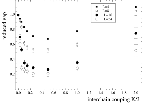
FIG. 3.: Results of a Quantum Monte Carlo simulation for the gap $\Delta$ divided by the $K=0$ value $\Delta_{0}$. The data are shown for $N=4$, 8, 16 and 24, where $N$ is the length of the ladder. $\Delta_{0}$ was also obtained from exact diagonalizations, when available.

In order to measure the spin excitation gap this way, one first finds the lowest energy level in the $S^{z}_{tot}=0$ sector, and then in the $S^{z}_{tot}=1$ sector. The difference should be equal to the gap $\Delta$. Notice that the unitary transformation (68) has effectively shifted the momentum of excitations by $\pi$, so that the first excited state of a Haldane system has now momentum zero and is not eliminated by projecting onto the uniform state $|\xi\rangle$.

The outcome of the simulation for the gap and the ground state energy per site as a function of $K$ is presented on Figs. 3 and 4. Notice that the gap exhibits a sharp drop until about $K\sim 0.5$, after which it rises slowly. We have not performed simulations on ladders longer than 24 rungs (48 sites), which is not enough to do a satisfactory finite-size analysis for most values of $K$. Nevertheless, we feel that the correct qualitative behavior as a function of $K$ may be extracted.

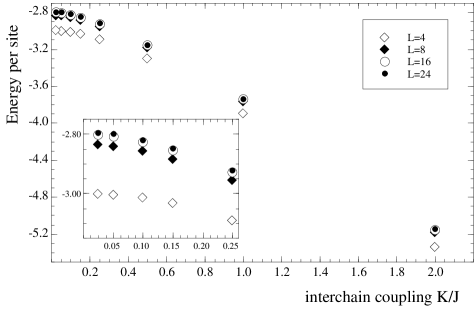
FIG. 4.: Results of a Quantum Monte Carlo simulation for the ground state energy per site $\varepsilon_{0}=E_{0}/N$, with $N=4$, 8, 16 and 24.

V Discussion

In the first part of this work we mapped the Hamiltonian of the Heisenberg ladder to the one-dimensional nonlinear sigma model, within the path integral formalism and the approximation of local AF order. From our knowledge of the nonlinear sigma model (with or without topological term), we concluded that the ladder has an excitation gap for all values of the inter-chain coupling $K$ if the spins $s$ and $\tilde{s}$ of the two chains are both integers, or both half-integers (i.e. if $s+\tilde{s}$ is an integer), whereas it has no gap if $s+\tilde{s}$ is a half-integer. In the former case, the ladder is in a Haldane phase for all nonzero values of $K$, positive or negative. This agrees with the interpretation of Ref. [9]

However, the quantitative estimate (45) of the gap $\Delta$ as a function of $K$, obtained via the saddle-point approximation of the nonlinear sigma model and illustrated on Fig. 1, is clearly wrong in both the $K\to 0$ and $K\to\infty$ limits. For small $K$, it announces a uniform increase of the gap from a finite value at $K=0$. In reality, the gap vanishes as $K\to 0$ if $s=\tilde{s}=\frac{1}{2}$, whereas it drops from its $K=0$ value if $s=\tilde{s}=1$.[2] Thus, there is a qualitative difference between half-integer and integer spin in the ladder when $K$ is small, as we naturally expect. This difference does not show up in the nonlinear sigma model representation of the ladder.

For large values of $K$, Eq. (45) predicts a square-root behavior $\sim\sqrt{K}$ when $K$ is large. In reality, the gap is approximately equal to $K$ in that limit, i.e., the energy difference between a singlet and a triplet on a single rung, when $J$ is neglected before $K$. In fact, we do not expect the parameters of the ladder non-linear sigma model of Sect. II to be correct when the ratio $K/J$ is too far from unity. However, for moderate values of $K$ ($0.5<K<2$), the gap of the spin-1 ladder illustrated in Fig. 3 shows a moderate increase whose slope is compatible with the estimate of Fig. 1.

The behavior of the ladder for small inter-chain coupling ($K\ll J$) is better represented by two interacting nonlinear sigma models. In the half-integer spin case, the presence of a topological term in each of the chain makes the analysis quite difficult; we hope to report on this in later work. However, the integer-spin case lends itself to a saddle-point evaluation of the gap which is much closer to reality. In the absence of variational principle or other guideline, it is difficult to say which of the two saddle-point methods illustrated on Fig. 2 offers a better estimate of the gap. A comparison with the Monte Carlo data of Fig. 3 tilts the balance in favor of the lower curve, which displays a sharper drop as $K$ increases from zero. Recall that the saddle-point approximation leading to this curve neglects the fluctuations of the mass matrix $\Sigma$ of Eq. (49), whereas the upper curve is obtained by neglecting the fluctuations of the Lagrange multipliers $\sigma_{i}$ of Eq. (48).

- [1] Choosing the same lattice spacing in the imaginary-time and space directions is somewhat arbitrary, but does the least violence to the Lorentz invariance of the theory.
- [2] If the numerical results of Ref. [7] for finite-length ladders were plotted in terms of , as in Fig. 3, we would observe a rise of the curve as the length increases, in contrast to Fig. 3.
- [3] F. D. M. Haldane, Phys. Lett. 93A, 464 (1983); Phys. Rev. Lett.50, 1153 (1983).
- [4] K. Hida, J. Phys. Soc. Jpn. 60, 1347 (1991).
- [5] S. P. Strong and A. J. Millis, Phys. Rev. Lett.69, 2419 (1992).
- [6] E. Dagotto, J. Riera and D. Scalapino, Phys. Rev. B45, 5744 (1992).
- [7] T. Barnes, E. Dagotto, J. Riera and E.S. Swanson, Phys. Rev. B47, 3196 (1993).
- [8] M. Azzouz, L. Chen and S. Moukouri, Phys. Rev. B50, 6233 (1994).
- [9] S. White, equivalence of the antiferromagnetic Heisenberg ladder to a single chain, University of California (Irvine) preprint.
- [10] M. P. Nightingale, H. W. J. Blöte, Phys. Rev. B33, 659 (1986).
- [11] M. Takahashi, Phys. Rev. Lett.62, 2313 (1989); M. Takahashi, Phys. Rev. B48, 311 (1993).
- [12] S. R. White, Phys. Rev. Lett.69, 2863 (1992); S. R. White and D. A. Huse, Phys. Rev. B48, 3844 (1993).
- [13] D. Sénéchal, Phys. Rev. B48, 15 880 (1993).
- [14] E. Fradkin, Field Theories of Condensed Matter Systems, Addison-Wesley, Reading, MA, 1991.
- [15] E. Manousakis, Rev. Mod. Phys. 63, 1 (1991).
- [16] I. Affleck, in Field Theory Methods and Quantum Critical Phenomena, Les Houches, session XLIX, 1988, Champs, Cordes et Phénomènes Critiques (Elsevier, New York, 1989).
- [17] L. Chen, private communication.
- [18] M. Takahashi, Phys. Rev. Lett.62, 2313 (1989).
- [19] J. H. Hetherington, Phys. Rev. A30, 2713 (1983).