ITP-UH-16/95 May 1995

cond-mat/9505146

On the Hubbard Model in the Limit of Vanishing Interaction

Holger Frahm and Markus P. Pfannmüller
Institut für Theoretische Physik, Universität Hannover
D-30167 Hannover, Germany
ABSTRACT

We address the question how a correspondence between the particle like excitations in the one dimensional Hubbard model (i.e. “holons” and “spinons”) and the free fermionic picture can be estabilished in the limit of vanishing interaction by studying the finite size spectrum in the framework of the Bethe Ansatz. Special attention has to be paid to the case of a vanishing magnetic field where the two bands of excitations in either description are degenerate. The interaction lifts this degeneracy.

PACS-numbers: 71.27.+a   75.10.Lp   05.70.Jk  

The Hubbard model is one of the most studied models for interacting electrons on a one-dimensional lattice. Following Lieb and Wu’s [1] Bethe Ansatz (BA) solution many exact results have been obtained. These provide detailed understanding of the thermodynamics [2], excitation spectrum [3]–[5], finite size corrections [6, 7] and asymptotics of correlation functions [8, 9] which are believed to show the generic behaviour of systems of interacting electrons in one spatial dimension.

The Hamiltonian is given in terms of standard fermionic creation resp. annihilation operators $\Psi^{\dagger}_{j,\sigma}$ and $\Psi_{j,\sigma}$ of electrons with spin $\sigma$ at site $j$ and the corresponding occupation numbers $n_{j,\sigma}=\Psi^{\dagger}_{j,\sigma}\Psi_{j,\sigma}$

$${\cal H}=\sum_{j=1}^{N}\Biggl{[}\,\sum_{\sigma=\uparrow,\downarrow}\left(\Psi^{\dagger}_{j+1,\sigma}\Psi_{j,\sigma}+\Psi^{\dagger}_{j,\sigma}\Psi_{j+1,\sigma}\right)+4u\,n_{j,\uparrow}n_{j,\downarrow}+\mu\,(n_{j,\uparrow}+n_{j,\downarrow})-\frac{h}{2}\,(n_{j,\uparrow}-n_{j,\downarrow})\Biggr{]}$$ (1)

where $u$ is the strength of the on-site Coulomb repulsion, $\mu$ the chemical potential and $h$ an additional external magnetic field. In the following we consider the repulsive case $u\geq 0$ with $h\geq 0\,$.

For vanishing coupling constant $u=0$ the model simply describes two independent generations of free fermions. This fact allows, of course, to extract the physical properties of the system in a much simpler way than through the BA. Nevertheless, there have been studies of the BA solution in the $u\to 0$ limit, mainly motivated by the desire to have a reliable test for perturbative schemes expanding around the free fermionic limit. These studies have mainly concentrated on the $u$-dependence of the ground state energy for the half-filled band, finding that the ground state energy can be expanded in an asymptotic series in $u$ which is reproduced correctly by standard perturbation theory [10]–[12].

In this letter we extend the study of the $u\to 0$ limit to include the behaviour of the low-lying excitations. In particular, we address the question how a correspondence between the particle like excitations of the interacting system (i.e. “holons” and “spinons”) as obtained from the BA and those present in the free fermion spectrum can be established in this limit. It turns out that in a finite magnetic field there is a one to one correspondence between the excitations in either description. In absence of a magnetic field the single particle energies of noninteracting spin-$\uparrow$ and spin-$\downarrow$ electrons are identical. This is reproduced by the BA solutions where the Fermi velocities of spin- and charge excitations are degenerate in the limit $u\to 0\,$. As a consequence both pictures lead to a correct description of the spectrum of (at least low-lying) excitations, charge an spin degrees of freedom can be assigned to the two degenerate bands of excitations in an almost arbitrary way. For finite values of $u$ this degeneracy is lifted. We investigate how the difference between the two velocities develops as a function of the interaction strength $u$ for zero magnetic field.

We recall that the density of charge and spin waves in the thermodynamic limit is given in terms of an inhomogeneous integral equation

$$\rho=\rho^{(0)}+\mbox{\boldmath$\hat{K}$}*\rho$$ (2)

where $\rho$ and $\rho^{(0)}$ are column vectors with entries

$$\rho={\rho_{c}(k)\choose\rho_{s}(\lambda)},\hskip 28.45274pt\rho^{(0)}={\frac{1}{2\pi}\choose 0}$$ (3)

and $\hat{K}$ is a $2\times 2$ matrix whose elements are integral operators, namely

$$\mbox{\boldmath$\hat{K}$}=\left(\begin{array}[]{cc}0&\cos k\int\limits_{-\lambda_{0}}^{+\lambda_{0}}d\lambda^{\prime}K_{1}(\sin k-\lambda^{\prime})*\rule[-22.76219pt]{0.0pt}{22.76219pt}\\ \int\limits_{-k_{0}}^{+k_{0}}dk^{\prime}K_{1}(\lambda-\sin k^{\prime})*&-\int\limits_{-\lambda_{0}}^{+\lambda_{0}}d\lambda^{\prime}K_{2}(\lambda-\lambda^{\prime})*\end{array}\right)\ .$$ (4)

The renormalized energies of the corresponding excitations read

$$\epsilon=\epsilon^{(0)}+\mbox{\boldmath$\hat{K}$}^{T}*\epsilon$$ (5)

with

$$\epsilon={\epsilon_{c}(k)\choose\epsilon_{s}(\lambda)}\ ,\hskip 28.45274pt\epsilon^{(0)}={\mu-\frac{h}{2}-2\cos k\choose h}\ .$$ (6)

The integral operator matrix $\mbox{\boldmath$\hat{K}$}^{T}$ is the transpose of $\hat{K}$, namely

$$\mbox{\boldmath$\hat{K}$}^{T}=\left(\begin{array}[]{cc}0&\int\limits_{-\lambda_{0}}^{+\lambda_{0}}d\lambda^{\prime}K_{1}(\sin k-\lambda^{\prime})*\rule[-22.76219pt]{0.0pt}{22.76219pt}\\ \int\limits_{-k_{0}}^{+k_{0}}dk^{\prime}\cos k^{\prime}K_{1}(\lambda-\sin k^{\prime})*&-\int\limits_{-\lambda_{0}}^{+\lambda_{0}}d\lambda^{\prime}K_{2}(\lambda-\lambda^{\prime})*\end{array}\right)\ .$$ (7)

In these equations the kernels $K_{1}$ and $K_{2}$ are given by

$$K_{1}(x)=\frac{1}{2\pi}\ \frac{2u}{u^{2}+x^{2}}\ ,\hskip 28.45274ptK_{2}(x)=\frac{1}{2\pi}\ \frac{4u}{4u^{2}+x^{2}}\ .$$ (8)

For a comparison to the free fermionic description the finite size corrections of the BA spectrum as calculated in [7] are particularly useful. The energies and momenta of the low lying excitations are given by

$$E-E_{0} = \frac{2\pi}{N}\Bigl{[}\frac{1}{4}\Delta N^{T}(\mbox{\boldmath$Z$}^{-1})^{T}\mbox{\boldmath$VZ$}^{-1}\Delta N+D^{T}\mbox{\boldmath$ZVZ$}^{T}D$$ (9)

$$+v_{c}(N^{+}_{c}+N^{-}_{c})+v_{s}(N^{+}_{s}+N^{-}_{s})\Bigr{]}+o\left(\frac{1}{N}\right)\ ,$$

$$P-P_{0} = \frac{2\pi}{N}(\Delta N^{T}D+N^{+}_{c}-N^{-}_{c}+N^{+}_{s}-N^{-}_{s})$$ (10)

$$+2D_{c}k_{F,\uparrow}+2(D_{c}+D_{s})k_{F,\downarrow}\ .$$

Here $V$ denotes the diagonal matrix $\mbox{\boldmath$V$}=\mbox{diag}(v_{c},v_{s})\,$ of the Fermi velocities of charge and spin waves

$$v_{c}=\frac{\epsilon^{\prime}_{c}(k_{0})}{2\pi\rho_{c}(k_{0})}\ ,\hskip 28.45274ptv_{s}=\frac{\epsilon^{\prime}_{s}(\lambda_{0})}{2\pi\rho_{s}(\lambda_{0})}\ .$$ (11)

The matrix

$$\mbox{\boldmath$Z$}=\left(\begin{array}[]{cc}Z_{cc}&Z_{cs}\\ Z_{sc}&Z_{ss}\end{array}\right)=\left(\begin{array}[]{cc}\xi_{cc}(k_{0})&\xi_{sc}(k_{0})\\ \xi_{cs}(\lambda_{0})&\xi_{ss}(\lambda_{0})\end{array}\right)^{T}$$ (12)

is given in terms of the dressed charge matrix $\xi$ which is defined by the integral equation

$$\mbox{\boldmath$\xi$}=\mbox{\boldmath$I$}+\mbox{\boldmath$\hat{K}$}^{T}*\mbox{\boldmath$\xi$}$$ (13)

where $I$ is the $2\times 2$ unit matrix. The vectors

$$\Delta N={\Delta N_{c}\choose\Delta N_{s}}\ ,\hskip 56.9055ptD={D_{c}\choose D_{s}}$$ (14)

and the positive integers $N^{\pm}_{c}$ and $N^{\pm}_{s}$ characterize the excited state. Here $\Delta N_{c}=\Delta N_{\uparrow}+\Delta N_{\downarrow}\,$ and $\Delta N_{s}=\Delta N_{\downarrow}\,$ are related to the change in particle numbers with respect to their ground state values thus determining charge and spin of the excitated state, respectively. $D_{c}=D_{\uparrow}\,$ and $D_{s}=D_{\downarrow}-D_{\uparrow}\,$ are given by the number of particles moved from the left to right Fermi points at $\pm k_{F,\sigma}=\pm\pi n_{\sigma}$ ($n_{\sigma}$ are the total densities of electrons with spin $\sigma$). Their values are integers or half integers subject to the conditions $D_{c}\equiv(\Delta N_{c}+\Delta N_{s})/2\,$ and $D_{s}\equiv\Delta N_{c}/2\,$ modulo $1$. The values of $N^{\pm}_{c,s}$ are the quantum numbers of particle–hole excitations at the right, resp. left Fermi points.

For vanishing $u$ the kernels (8) become $\delta$-functions and the solution of Eqs. (2), (5), (13) is trivial. However, to determine the Fermi velocities (11) and the matrix $Z$ (12) these solutions have to be taken at the boundaries $k_{0}\,$ and $\lambda_{0}\,$. For $\sin k_{0}\leq\lambda_{0}\,$ the solutions are discontinuous at these points and the limit $u\to 0$ has to be performed after solving the integral equations.

To see whether this situation can arise we restrict ourselves to $\lambda_{0}<\sin k_{0}$ first. In this case the discontinuities are moved away from the boundaries entering (11) and (12) and we find

$$\rho_{c}(k) = \left\{\begin{array}[]{ccl}\frac{1}{\pi}&\mbox{ if }&0\leq|k|\leq\arcsin\lambda_{0}\\ \frac{1}{2\pi}&\mbox{ if }&\arcsin\lambda_{0}<|k|\end{array}\right.\ ,$$ (17)

$$\rho_{s}(\lambda) = \left\{\begin{array}[]{ccl}\frac{1}{2\pi\cos(\arcsin\lambda)}&\mbox{ if }&0\leq|\lambda|\leq\sin k_{0}\\ 0&\mbox{ if }&\sin k_{0}<|\lambda|\end{array}\right.\ .$$ (20)

(Alternatively one can express the density $\rho_{s}$ as a function of quasimomenta $k=\arcsin\lambda\,$ rather than the rapidities $\lambda$ themselves, (20) simplifies to $\rho_{s}(k)=\theta(k_{0}-|k|)/(2\pi)$.) From these equations we obtain for the total densities of the charge and spin excitations corresponding to this state

$$n_{c}=\int_{-k_{0}}^{+k_{0}}\rho_{c}(k)\,dk\;=\;\frac{k_{0}}{\pi}+\frac{\arcsin\lambda_{0}}{\pi}\ ,\qquad n_{s}=\int_{-\lambda_{0}}^{+\lambda_{0}}\rho_{s}(\lambda)\,d\lambda\;=\;\frac{\arcsin\lambda_{0}}{\pi}$$ (21)

which allows for the identification of $k_{0}\,$ and $\lambda_{0}\,$ in terms of the Fermi momenta through $k_{0}=k_{F,\uparrow}\,$ and $\arcsin\lambda_{0}=k_{F,\downarrow}\,$. Thus we find that the condition $\lambda_{0}<\sin k_{0}\,$ is satisfied for any $h>0$. The case of a vanishing magnetic field has to treated separately.

The dressed energies are given by

$$\epsilon_{c}(k) = \left\{\begin{array}[]{ccl}2\mu-4\cos k&\mbox{ if }&0\leq|k|\leq\arcsin\lambda_{0}\\ \mu-\frac{h}{2}-2\cos k&\mbox{ if }&\arcsin\lambda_{0}<|k|\end{array}\right.\ ,$$ (24)

$$\epsilon_{s}(k) = \left\{\begin{array}[]{ccl}\mu+\frac{h}{2}-2\cos k&\mbox{ if }&0\leq|k|\leq k_{0}\\ h&\mbox{ if }&k_{0}<|k|\end{array}\right.\ .$$ (27)

From Eq. (11) we find $v_{c}=2\sin(k_{F,\uparrow})$ and $v_{s}=2\sin(k_{F,\downarrow})\,$. Similarly the result for the dressed charge matrix gives

$$\mbox{\boldmath$Z$}=\left(\begin{array}[]{cc}1&1\\ 0&1\end{array}\right)\ .$$ (28)

Now comparing the finite size corrections for the excited states (9) with this expression for the matrix $Z$ and the corresponding free fermion result the two are found to agree.

The case of a vanishing magnetic field $h=0$ needs a special treatment. In this case we have $\lambda_{0}=\infty$ and the dressed charge matrix can be expressed in terms of a single quantitity $\xi$ [7]

$$\mbox{\boldmath$\xi$}=\left(\begin{array}[]{cc}\xi(z)&0\\ \frac{1}{2}\xi(z)&\frac{1}{\sqrt{2}}\end{array}\right)$$ (29)

satisfying the integral equation

$$\xi(z)=1+\int^{z_{0}}_{-z_{0}}K(z-z^{\prime})\xi(z^{\prime})dz^{\prime}$$ (30)

with the kernel

$$K(x)=\frac{1}{2\pi}\int_{0}^{\infty}\frac{e^{-\omega}}{\cosh(\omega)}\cos(\omega x)d\omega$$ (31)

and $z=\sin k/u\,$. For large $z_{0}=\sin k_{0}/u$ the quantity $\xi(z_{0})$ entering (12) can be obtained using a perturbative scheme based on the Wiener–Hopf method [13]. The result to order $1/z_{0}$ reads [8]

$$\xi(z_{0})=\sqrt{2}\left(1-\frac{1}{2\pi z_{0}}\right)\ .$$ (32)

In the limit $u\rightarrow 0$ we find the following dressed charge matrix

$$\mbox{\boldmath$Z$}=\left(\begin{array}[]{cc}\sqrt{2}&0\\ \frac{1}{2}{\sqrt{2}}&\frac{1}{2}{\sqrt{2}}\end{array}\right)\ .$$ (33)

One might have expected that the result (28) for $Z$ holds even for a vanishing magnetic field as there is no dependence on $h$. This is indeed the case. “Holons” and “spinons” are certain combinations of spin-$\uparrow$ and spin-$\downarrow$ electrons. For vanishing magnetic field these combinations become arbitrary since spin-$\uparrow$ and spin-$\downarrow$ electrons have equal energies. The Fermi velocities are equal, $v_{c}=v_{s}=2\sin k_{F}$, and thus the matrix $V$ is proportional to the unit matrix, $\mbox{\boldmath$V$}=\,2\sin(k_{F}){1\,0\choose 0\,1}\,$. Of physical relevance are only the combinations $(\mbox{\boldmath$Z$}^{-1})^{T}\mbox{\boldmath$VZ$}^{-1}$ and $\mbox{\boldmath$ZVZ$}^{T}$ which enter expression (9) for the excited states. For both choices of $Z$ the results coincide.

The degeneracy of the Fermi velocities of charge and spin wave exciations is lifted by the interaction. Using (11) the Fermi velocities for $h=0$ can be expressed as

$$v_{c}={1\over 2\pi}\ \frac{g(z_{0})}{f(z_{0})}\ ,\qquad v_{s}={1\over 2\pi}\ \frac{\int^{z_{0}}_{-z_{0}}e^{\frac{\pi}{2}z}g(z)dz}{\int^{z_{0}}_{-z_{0}}e^{\frac{\pi}{2}z}f(z)dz}\ .$$ (34)

Here $f(z)$ and $g(z)$ are are the density $\rho_{c}$ and the derivative of the dressed energy $\epsilon^{\prime}_{c}$ as a function of the variable $z$ given in terms of the following integral equations (remember that we have $uz=\sin k<1$)

$$f(z) = \frac{1}{2\pi\sqrt{1-u^{2}z^{2}}}+\int^{z_{0}}_{-z_{0}}K(z-z^{\prime})f(z^{\prime})dz^{\prime}\ ,$$

$$g(z) = \frac{2uz}{\sqrt{1-u^{2}z^{2}}}+\int^{z_{0}}_{-z_{0}}K(z-z^{\prime})g(z^{\prime})dz^{\prime}$$ (35)

with the kernel $K$ given by Eq. (31). Again, the quantities necessary to compute the Fermi velocities (34) for small $u$, i.e. $z_{0}\approx\infty\,$, can be obtained from these equations using the Wiener-Hopf method. A complication is given by the explicit $u$–dependence of the driving terms. However, for small densities (i.e. $uz_{0}=\sin k_{0}\ll 1$) they can be expanded up to linear order in $uz$. For $f$ this results in Eq. (30) for the dressed charge $\xi$ (up to a factor of $1/2\pi$). In the equation for $g$ the driving term is replaced by $2uz$. For $0<u\ll\sin(k_{0})<1$ we finally get the following result for the Fermi velocities

$$v_{c} = 2u\left[z_{0}-\frac{1}{\pi}\ln(z_{0})+\frac{1}{\pi}\ln\left(\frac{2}{\pi}\right)\right]\ ,$$

$$v_{s} = 2u\left[z_{0}-\frac{1}{\pi}\ln(z_{0})+\frac{1}{\pi}\ln\left(\frac{2}{\pi}\right)-\frac{2}{\pi}\right]\ .$$ (36)

The leading term $2uz_{0}\,$ is simply the free fermion result $2\sin k_{0}\,$. The logarithmic corrections $\propto u\ln u$ are probably just a consequence of the expression of the velocities in terms of $z_{0}\,$ rather than the electron density $n_{c}\,$. To prove this analytically the Wiener-Hopf scheme mentioned above has to be performed to order $z_{0}^{-2}$ which raises questions in its quality. However, numerical solution of the integral equations (35) suggests the absence of logarithmic corrections in $v_{\alpha}(n_{c},u)$. In Fig. 1 we present the Fermi velocities for a fixed value of $\sin k_{0}=0.1$ which are computed from the numerical solution of the integral equations (35) in comparison with Eqs. (36). Because of the various approximations which were necessary to derive Eqs. (36) we expect the results only do be correct up to the order of $u$.

An interesting observation is that, in leading order, the gap between charge and spin wave excitations is a linear function of the interaction $u$

$$v_{c}-v_{s}=\frac{4u}{\pi}\ .$$ (37)

Fig. 2 shows the difference of the Fermi velocities as a function of the total density of particles for various values of $u$. As for Fig. 1 the data were computed from numerical solutions of the integral equations. As long as $\rho$, i.e. $\sin k_{0}\,$, is not to small, we find exactly the behaviour as predicted by Eq. (37). For $\rho\rightarrow 0$ at fixed $u$ one has $z_{0}\rightarrow 0$ which allows to solve Eqs. (35) by iteration.

In this letter we have extended previous studies of the ground state properties of the one dimensional Hubbard model for small interaction $u$ to the low-lying excitations. Apart from providing the possibility for a check of perturbative methods our results emphasize the importance of the “spinon-holon” picture for strongly correlated electrons in particular in the case of a vanishing magnetic field.

This work has been supported in part by the Deutsche Forschungsgemeinschaft under Grant No. Fr 737/2–1.

Figures

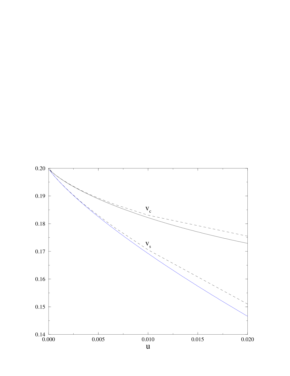
Figure 1: Fermi velocities for $h=0$ and $\sin k_{0}=0.1$ as a function of $u$. Solid lines correspond to numerical solutions of the integral equations (35), dashed lines to the asymptotic expressions (36).

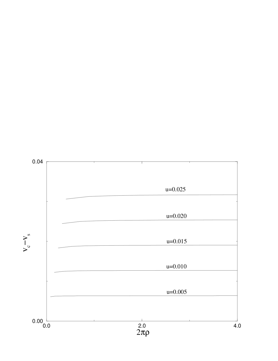
Figure 2: Difference of Fermi velocities for $h=0$ as a function of the total density computed from numerical solutions of Eqs. (35).

References

• [1] E. H. Lieb and F. Y. Wu, Phys. Rev. Lett. 20 (1968) 1445.
• [2] M. Takahashi, Prog. Theor. Phys. 47 (1972) 69.
• [3] A. A. Ovchinnikov, Sov. Phys. JETP 30 (1970) 1160.
• [4] C. F. Coll, III, Phys. Rev. B 9 (1974) 2150.
• [5] F. H. L. Eßler and V. E. Korepin, Nucl. Phys. B 426 (1994) 505.
• [6] F. Woynarovich and H.-P. Eckle, J. Phys. A 20 (1987) L443.
• [7] F. Woynarovich, J. Phys. A 22 (1989) 4243.
• [8] H. Frahm and V. E. Korepin, Phys. Rev. B 42 (1990) 10553.
• [9] H. Frahm and V. E. Korepin, Phys. Rev. B 43 (1991) 5653.
• [10] M. Takahashi, Progr. Theor. Phys. 45 (1971) 756.
• [11] E. N. Economou and P. N. Poulopoulos, Phys. Rev. B 20 (1979) 4756.
• [12] W. Metzner and D. Vollhardt, Phys. Rev. B 39 (1989) 4462.
• [13] C. N. Yang and C. P. Yang, Phys. Rev. 150 (1966) 327.