[

Renormalization group study of interacting electrons

The renormalization-group (RG) approach proposed earlier by Shankar for interacting spinless fermions at $T=0$ is extended to the case of non-zero temperature and spin. We study a model with $SU(N)$-invariant short-range effective interaction and rotationally invariant Fermi surface in two and three dimensions. We show that the Landau interaction function of the Fermi liquid, constructed from the bare parameters of the low-energy effective action, is RG invariant. On the other hand, the physical forward scattering vertex is found as a stable fixed point of the RG flow. We demonstrate that in $d=2$ and 3, the RG approach to this model is equivalent to Landau’s mean-field treatment of the Fermi liquid. We discuss subtleties associated with the symmetry properties of the scattering amplitude, the Landau function and the low-energy effective action. Applying the RG to response functions, we find the compressibility and the spin susceptibility as fixed points.

]

I Introduction

The necessity to better understand the Physics of strongly correlated fermions, like in high-$T_{c}$ superconductors or in the fractional quantum Hall effect, inspired a lot of theoretical efforts to explain the observable deviations from Fermi liquid (FL) behavior, and to clarify the foundations of the Landau Fermi liquid theory itself. Much work has been done to elucidate the microscopic basis of the FL theory in the framework of quantum field theory[4, 5]. However, the development of Renormalization Group (RG) methods to the problem of interacting fermions in dimension $d$ is relatively new.

So far, the most successful applications of RG methods to interacting fermions have been achieved in the one-dimensional case, where it was known from exact solutions that non FL phases exist (e.g. the Luttinger liquid). For a review on 1D systems see Ref. [6]. Later, Bourbonnais and Caron[7] made an extensive RG study of one-dimensional and quasi-one-dimensional fermion systems at finite temperature, in which a transition from Luttinger liquid to FL behavior is revealed. The development of a RG theory for interacting fermions in isotropic systems of dimensions greater than one is more recent[8, 9, 10, 11]. Such a generic theory, when completed, should include the Landau FL theory as one of the fixed points of the RG equations. As discussed by Shankar in a very pedagogical paper,[11] the RG treatment of fermions is a much more complicated issue than the analogous procedure for critical phenomena, because of two crucial points: Firstly, the existence of a Fermi surface: the low-energy modes lie in the vicinity of a continuous geometrical object (the Fermi surface) and not only around isolated points, like the origin of phase space in the bosonic case. This introduces additional phase space constraints on the modes to be integrated out, quite a problem for an arbitrary Fermi surface. Moreover, the Fermi surface itself is a relevant parameter of theory, and its shape should renormalize under the RG procedure, except in the rotationally symmetric case. Secondly, instead of studying the flow of one or a few coupling constants like in critical phenomena, one has to set up RG flow equations for coupling functions, defined on the Fermi surface. Notice that the purely 1D interacting fermion system can be considered as a degenerate special case where the Fermi surface is reduced to a set of two points, with a finite number of coupling constants. It is therefore closer to the usual applications of the renormalization group (however, in the quasi-one-dimensional approach of Ref. [7], one already witnesses the appearance of new coupling constants related to interchain hopping and one may follow the change in shape of the (open) Fermi surface under RG flow).

In this paper we extend Shankar’s approach[11], developed for spinless fermions at zero temperature. The main goal of our analysis is to incorporate spin and a finite temperature. For the sake of generality, we study a system of $N$-component fermions with an $SU(N)$-invariant short-range interaction. We perform the analysis for a circular Fermi surface in dimension two, spherical in dimension three.

Shankar’s analysis of coupling functions for the quartic interaction shows that only two such functions survive under the RG flow: the function $\hat{\Phi}$, which couples two incoming and two outgoing particles with the same pairs of momenta lying on the Fermi surface (Landau channel), and the function $\hat{V}$, which couples incoming and outgoing particles with opposite momenta lying on the Fermi surface (Bardeen-Cooper-Schrieffer (BCS) channel).

We find that the coupling function $\hat{V}$ is marginally irrelevant if its bare value satisfies Landau’s conditions for the stability of the Fermi liquid against Cooper pairing at arbitrary momentum; otherwise a BCS instability occurs at finite temperature. In the Landau channel the distinction between the Landau interaction function $\hat{\Phi}$ and the physical forward scattering vertex $\hat{\Gamma}$ appears naturally in the finite temperature RG formalism. The function $\hat{\Phi}$ is RG invariant at non-zero temperatures, while the vertex $\hat{\Gamma}$ is attracted towards a non trivial stable fixed point. In order for the Fermi liquid to be stable up to zero temperature, we find that the components of the Landau function must obey conditions which coincide with Pomeranchuk’s stability conditions.[13]

The paper is organized as follows: In Section II we describe the low-energy effective action which is the starting point of our RG analysis. In Section III we study the two-dimensional case. This section contains a description of the key points of our analysis and most of the technical details. There, we obtain the RG equations for the vertices and their fixed points. In Section IV we apply the same analysis to $d=3$. In Section V we calculate the compressibility and the spin susceptibility in this RG framework.

II The low-energy effective action

We treat the problem of interacting fermions at finite temperature in the standard path integral formalism[14] using Grassmann variables for Fermi fields. The partition function is given by the path integral

$$Z=\int{\cal D}\bar{\psi}{\cal D}\psi~{}e^{S_{0}+S_{int}}$$ (1)

wherein the free part of the action is

$$S_{0}=\int_{({\bf 1})}\bar{\psi}_{\alpha}({\bf 1})\left[i\omega_{1}+\mu-\epsilon({\bf K}_{1})\right]\psi_{\alpha}({\bf 1})$$ (2)

We introduced the following notation:

$$\int_{({\bf i})}~{}~{} \equiv ~{}~{}{1\over\beta}\int{d{\bf K}_{i}\over(2\pi)^{d}}\sum_{\omega_{i}}$$ (4)

$$({\bf i})~{}~{} \equiv ~{}~{}({\bf K}_{i},\omega_{i})$$ (5)

where $\beta$ is the inverse temperature, $\mu$ the chemical potential, $\omega_{i}$ the fermion Matsubara frequencies and $\psi_{\alpha}({\bf i})$ an $N$-component Grassmann field with a ‘flavor’ index $\alpha$. Summation over repeated indices is implicit throughout this paper. We set $k_{B}=1$ and $\hbar=1$. The physically interesting case is of course $N=2$, but the generalization to $N\neq 2$ is simple, and it incorporates automatically the simpler case of spinless fermions ($N=1$).

The general $SU(N)$-invariant quartic interaction may be written as follows:

$$S_{int} = -\frac{1}{4}\int_{({\bf 1},{\bf 2},{\bf 3},{\bf 4})}\bar{\psi}_{\alpha}({\bf 1})\bar{\psi}_{\beta}({\bf 2})\psi_{\gamma}({\bf 3})\psi_{\delta}({\bf 4})$$ (7)

$$\times U^{\alpha\beta}_{\gamma\delta}({\bf 1},{\bf 2};{\bf 3},{\bf 4})\delta^{(d+1)}({\bf 1}+{\bf 2}-{\bf 3}-{\bf 4})$$

Here the conservation of energy and momentum is enforced by the symbolic delta function

$$\delta^{(d+1)}({\bf 1}+{\bf 2}-{\bf 3}-{\bf 4})\equiv\beta(2\pi)^{d}\times$$ (8)

$$\delta({\bf K}_{1}+{\bf K}_{2}-{\bf K}_{3}-{\bf K}_{4})\Delta(\omega_{1}+\omega_{2}-\omega_{3}-\omega_{4})$$ (9)

where the discrete delta function $\Delta$ is equal to 1 if its argument is zero, and equal to zero otherwise.

It can be shown in group theory (see, for instance, Ref. [15]) that a representation of the potential as

$$U^{\alpha\beta}_{\gamma\delta}=U_{1}\delta_{\alpha\delta}\delta_{\beta\gamma}+U_{2}\sum_{a=1}^{N^{2}-1}\lambda^{a}_{\alpha\delta}\lambda^{a}_{\beta\gamma}$$ (10)

supplies us with the most general $SU(N)$-invariant form with two independent scalar functions $U_{1}$ and $U_{2}$. The $N^{2}-1$ Hermitian traceless matrices $\hat{\lambda}^{a}$ are the generators of $SU(N)$. We need not write down explicit expressions of the commutations or other relations for those matrices. The only identity used in the following is

$$\sum_{a=1}^{N^{2}-1}\lambda^{a}_{\alpha\beta}\lambda^{a}_{\gamma\delta}=2\left(\delta_{\alpha\delta}\delta_{\beta\gamma}-{1\over N}\delta_{\alpha\beta}\delta_{\gamma\delta}\right)$$ (11)

In the $SU(2)$ case, the three generators $\lambda^{a}$ are the usual Pauli matrices and the identity (11) reduces to a well-known relation involving these matrices. Using the relation (11), one readily checks that the form (10) of the interaction is indeed $SU(N)$ invariant. The fact that Eq. (10) is the most general $SU(N)$ invariant may be verified by counting the number of singlets in the tensor product $\bar{N}\otimes\bar{N}\otimes N\otimes N$, wherein $N$ stands for the fundamental representation of $SU(N)$ (acting on the $N$-component field $\psi$) and $\bar{N}$ for its conjugate. This number is indeed two, meaning that only two $SU(N)$-invariant scalars may be constructed in this way.

One should bear in mind the difference between the $SU(N)$-invariant interaction considered here and a rotation invariant interaction for particles of spin $s$: In the absence of symmetry-breaking interactions (e.g. spin-orbit, dipole-dipole, or external fields) there will be rotational invariance in spin space, but the corresponding symmetry operations are still obtained from the three generators of $SU(2)$, although in a $(2s+1)$-dimensional representation. The $SU(N)$-invariance imposed here is more stringent. The particular form of Eqs. (10,11), and consequently of Eq. (25), for any $N$, is the artifact of such a symmetry enlargement. A generic, $SU(2)$-invariant interaction with spin-$s$ fermions would contain a greater variety of terms. Accordingly, the different components of $\psi$ are called ‘flavors’ if $N=2s+1>2$, in order to avoid misunderstandings.

The flavor dependence of the potential (10) may be factorized and expressed via two independent flavor operators. It is convenient to introduce two operators $\hat{I}$ and $\hat{T}$, respectively symmetric and antisymmetric, as follows:

$$I^{\alpha\beta}_{\gamma\delta}~{} \equiv ~{}\delta_{\alpha\delta}\delta_{\beta\gamma}+\delta_{\alpha\gamma}\delta_{\beta\delta}$$ (13)

$$T^{\alpha\beta}_{\gamma\delta}~{} \equiv ~{}\delta_{\alpha\delta}\delta_{\beta\gamma}-\delta_{\alpha\gamma}\delta_{\beta\delta}$$ (14)

These operators satisfy the properties

$$I^{\alpha\beta}_{\gamma\delta} = \phantom{-}I^{\beta\alpha}_{\gamma\delta}=\phantom{-}I^{\alpha\beta}_{\delta\gamma}$$ (16)

$$T^{\alpha\beta}_{\gamma\delta} = -T^{\beta\alpha}_{\gamma\delta}=-T^{\alpha\beta}_{\delta\gamma}$$ (17)

and the convolution relations

$$I^{\alpha\beta}_{\mu\nu}I^{\nu\mu}_{\gamma\delta} = 2I^{\alpha\beta}_{\gamma\delta}$$ (19)

$$T^{\alpha\beta}_{\mu\nu}T^{\nu\mu}_{\gamma\delta} = 2T^{\alpha\beta}_{\gamma\delta}$$ (20)

$$T^{\alpha\beta}_{\mu\nu}I^{\nu\mu}_{\gamma\delta} = 0$$ (21)

$$I^{\alpha\mu}_{\gamma\nu}I^{\nu\beta}_{\mu\delta} = \phantom{-}{N+3\over 2}I^{\alpha\beta}_{\gamma\delta}-{N+1\over 2}T^{\alpha\beta}_{\gamma\delta}$$ (22)

$$I^{\alpha\mu}_{\gamma\nu}T^{\nu\beta}_{\mu\delta} = -{N-1\over 2}I^{\alpha\beta}_{\gamma\delta}+{N+1\over 2}T^{\alpha\beta}_{\gamma\delta}$$ (23)

$$T^{\alpha\mu}_{\gamma\nu}T^{\nu\beta}_{\mu\delta} = \phantom{-}{N-1\over 2}I^{\alpha\beta}_{\gamma\delta}-{N-3\over 2}T^{\alpha\beta}_{\gamma\delta}$$ (24)

Instead of Eq. (10), we may decompose the potential as follows:

$$U^{\alpha\beta}_{\gamma\delta}=U^{A}I^{\alpha\beta}_{\gamma\delta}+U^{S}T^{\alpha\beta}_{\gamma\delta}$$ (25)

where the functions $U^{S}$ and $U^{A}$ have the symmetry properties

$$U^{A}({\bf 1},{\bf 2};{\bf 3},{\bf 4}) = -U^{A}({\bf 2},{\bf 1};{\bf 3},{\bf 4})=-U^{A}({\bf 1},{\bf 2};{\bf 4},{\bf 3})$$ (27)

$$U^{S}({\bf 1},{\bf 2};{\bf 3},{\bf 4}) = \phantom{-}U^{S}({\bf 2},{\bf 1};{\bf 3},{\bf 4})=\phantom{-}U^{S}({\bf 1},{\bf 2};{\bf 4},{\bf 3})$$ (28)

The general form (7) of the interaction allows us to easily recover various special cases. Spinless fermions correspond to $N=1$: matrices have only one component and $\hat{I}\equiv 2$, $\hat{T}\equiv 0$. Thus there is only one interaction function. For instance, in the spinless Hubbard model with nearest-neighbor interaction constant $U^{nn}_{0}$, the function $U^{A}$ is expressed in terms of $U^{nn}_{0}$ and some combination of trigonometric functions, depending on the spatial dimension[11].

In the electron Hubbard model with on-site interaction constant $U^{os}_{0}$, the functions are $U^{A}=0$ and $U^{S}\propto U^{os}_{0}$. Switching on a constant interaction $U^{nn}_{0}$ between nearest neighbors, we come up with two independent functions $U^{S}$ and $U^{A}$ in the Hamiltonian.

The expressions (2) and (7) for the action are adequate for a microscopic, ‘exact’ formulation of the problem. The functions $U^{A}$ and $U^{S}$ may incorporate the microscopic interaction of our choice: Coulomb, on-site repulsion, and so on. The integration in Eq. (2) is then carried over all available phase space (the Brillouin zone), with the constraint of momentum conservation. In principle, working with the microscopic Hamiltonian allows a description of physical processes at all energy scales, up to atomic energies. However, such an exact solution is impossible in practice. We will consider the action defined in Eqs.(2,7) as a low-energy effective action[10, 11, 12], describing correctly only those physical processes occurring at an energy scale $\Lambda_{0}$ much smaller than the Fermi energy:

$$\Lambda_{0}\ll K_{F}$$ (29)

In principle, such a low-energy effective action could be obtained from the microscopic action by integrating out (in the functional sense) the degrees of freedom associated with the momenta lying out of a band of width $2\Lambda_{0}$ around the Fermi surface.

In general, the low-energy effective action $S_{0}+S_{int}$ is written as an expansion in a set of Grassmann fields, with the requirements that the symmetries of the microscopic action be satisfied (for details, see Refs. [10, 11]). We assume that the effective action has the form given in Eqs (2) and (7), except that the integration in Eq. (2) is restricted to the vicinity of the Fermi surface. The parameters of this action, like one-particle energy $\epsilon(\bf K)$ and the coupling functions $U^{A}$ and $U^{S}$, do not coincide with those of the microscopic action in general. We ignore the possibility of interaction terms involving derivatives, or more powers of $\psi$, because such terms are irrelevant at tree-level (see below).

In this work we will restrict ourselves to the study of low-density electron systems, so we assume that the Fermi surfaces have rotational symmetry (i.e. circular or spherical). The low-lying one-particle excitations can then be linearized near the Fermi energy in a simple fashion:

$$\epsilon({\bf K})-\mu\approx v_{F}(K-K_{F})\equiv v_{F}k$$ (30)

wherein the terms of order $k^{2}$ in this expansion are irrelevant. The momentum $k$ and the temperature $T$ are restricted by the inequalities $|k|\leq\Lambda_{0}$ and $T\ll v_{F}\Lambda_{0}$ along with the condition (29). The bare one-particle Green’s function for the free part of action $S_{0}$ is

$$\langle\psi_{\alpha}({\bf 1})\bar{\psi}_{\beta}({\bf 2})\rangle_{0} = G_{0}({\bf K}_{1},\omega_{1})\delta^{(d+1)}({\bf 1}-{\bf 2})\delta_{\alpha\beta}$$ (31)

$$G_{0}^{-1}({\bf K}_{1},\omega_{1}) = i\omega_{1}+\mu-\epsilon({\bf K}_{1})\simeq i\omega_{1}-v_{F}k_{1}$$ (32)

In the $d$-dimensional integration measure only the relevant term is kept:

$$\int d{\bf K} ~{}=~{} \int_{-\Lambda_{0}}^{\Lambda_{0}}\int_{\Omega_{d}}{(K_{F}+k)}^{d-1}dkd\Omega_{d}$$ (33)

$$~{}\simeq~{} K_{F}^{d-1}\int_{-\Lambda_{0}}^{\Lambda_{0}}\int_{\Omega_{d}}dkd\Omega_{d}$$ (34)

The Matsubara frequencies are allowed to run over all available values. We presume that the density of particles in the system is kept fixed.

The low-energy effective action (2,7) lends itself to a simple tree-level scaling analysis (dimensional analysis). It is invariant under the rescaling $\omega_{n}^{\prime}=s\omega_{n}$, $k^{\prime}=sk$ and $\psi^{\prime}(k^{\prime},\omega^{\prime}_{n})=s^{-3/2}\psi(k,\omega_{n})$. Higher orders in the expansion (30) or in the measure (33) are then irrelevant (in the RG sense) at tree-level, and so are more complicated interaction monomials. This justifies the simple form (2,7).

According to the RG analysis of Shankar[11], performed at zero temperature, this effective action describes the Fermi liquid phase of repelling spinless fermions and the BCS superconducting phase of attracting spinless fermions. We will study here the RG fixed points for interacting $N$-flavor fermions expanding this technique for the finite temperature case.

III The RG equations in two dimensions

A The coupling functions

In this section we will restrict the analysis to the two-dimensional case, with a circular Fermi surface. As follows from tree-level scaling, the frequency dependence of the coupling function $\hat{U}$ is irrelevant and is discarded from now on.

Each vector ${\bf K}_{i}$ in the effective action lies in a narrow shell of thickness $2\Lambda_{0}$ around the Fermi surface. We may write it as ${\bf K}_{i}={\bf K}_{F}^{i}+{\bf k}_{i}$ where the vector ${\bf k}_{i}$ is orthogonal to the Fermi surface and small, in the sense that $|{\bf k}_{i}|\leq\Lambda_{0}\ll K_{F}$. The coupling function is then written as

$$U^{A,S}=U^{A,S}({\bf K}_{F}^{1},{\bf K}_{F}^{2};{\bf K}_{F}^{3},{\bf K}_{F}^{4}|{\bf k}_{1},{\bf k}_{2};{\bf k}_{3},{\bf k}_{4})$$ (35)

If we restrict ourselves to the case of non-singular interactions,[17] the $\bf k$-dependence of the coupling function turns out to be irrelevant. Moreover, the dependence of the coupling function on the Fermi surface momenta ${\bf K}_{i}$ is constrained by crystal momentum conservation: ${\bf K}_{F}^{1}+{\bf K}_{F}^{2}={\bf K}_{F}^{3}+{\bf K}_{F}^{4}$ (we assumed that Umklapp processes are inoperative, which is justified for a circular Fermi surface at low-filling).

A geometrical analysis (see Ref.[11]) leads to the following conclusion: In the case of a circular Fermi surface, the constraint that the momenta ${\bf K}_{F}^{i}$ lie on the Fermi surface and the momentum conservation law allow the existence of two pairs of independent coupling functions, as described below.

Case 1.  If ${\bf K}_{F}^{1}\neq-{\bf K}_{F}^{2}$, we define a dimensionless coupling function $\hat{\Phi}$ of the momenta and spins:

$$\hat{\Phi}({\bf K}_{F}^{1},{\bf K}_{F}^{2})\equiv\frac{1}{2}\nu_{F}U^{\alpha\beta}_{\gamma\delta}({\bf K}_{F}^{1},{\bf K}_{F}^{2};{\bf K}_{F}^{1},{\bf K}_{F}^{2})$$ (36)

where $\nu_{F}=2S_{d}K_{F}^{d-1}/{(2\pi)}^{d}v_{F}$ is the density of electron states at the Fermi level and $S_{d}$ is the area of the $d$-dimensional unit sphere. The hat ($\hat{~{}}$) means that $\hat{\Phi}$ is an operator in flavor space. Each vector ${\bf K}_{F}^{a}$ may be specified by a plane polar angle $\theta_{a}$; because of rotation invariance, the function $\hat{\Phi}$ may only depend on the relative angle $\theta_{1}-\theta_{2}$ between ${\bf K}_{F}^{1}$ and ${\bf K}_{F}^{2}$:

$$\hat{\Phi}(\theta_{1}-\theta_{2})~{}=~{}\Phi^{A}(\theta_{1}-\theta_{2})I^{\alpha\beta}_{\gamma\delta}~{}+~{}\Phi^{S}(\theta_{1}-\theta_{2})T^{\alpha\beta}_{\gamma\delta}$$ (37)

It should be pointed out that the function $\Phi^{A}(\theta)$ is not an antisymmetric function of its argument. It follows from the symmetry properties of the coupling function (Eqs. (II,25,25)) that

$$\Phi^{A,S}(\theta_{1}-\theta_{2})=\Phi^{A,S}(\theta_{2}-\theta_{1})$$ (38)

The only remnant of the antisymmetry of $U^{A}$ is the condition $\Phi^{A}(0)=0$. It is easy to check that an exchange of incoming or outgoing momenta does not require any new independent function.

Case 2.  The two outgoing momenta are opposite: ${\bf K}_{F}^{2}=-{\bf K}_{F}^{1}$ (likewise for the two incoming momenta). We introduce another pair of dimensionless functions:

$$\hat{V}({\bf K}_{F}^{1},{\bf K}_{F}^{3}) \equiv \frac{1}{2}\nu_{F}U^{\alpha\beta}_{\gamma\delta}({\bf K}_{F}^{1},-{\bf K}_{F}^{1};{\bf K}_{F}^{3},-{\bf K}_{F}^{3})$$ (40)

$$= V^{A}(\theta_{13})I^{\alpha\beta}_{\gamma\delta}+V^{S}(\theta_{13})T^{\alpha\beta}_{\gamma\delta}$$ (41)

wherein $\theta_{13}\equiv\theta_{1}-\theta_{3}$. From the symmetry properties of the coupling function $\hat{U}$ under exchange of momenta, we find

$$V^{A}(\theta\pm\pi) = -V^{A}(\theta)$$ (43)

$$V^{S}(\theta\pm\pi) = \phantom{-}V^{S}(\theta)$$ (44)

There is an overlap in the definitions of $\hat{\Phi}$ and $\hat{V}$, since $\hat{\Phi}(\pm\pi)={\hat{V}}(0)$ or, more explicitly,

$$\Phi^{A}(\pm\pi)=V^{A}(0) = -V^{A}(\pm\pi)$$ (46)

$$\Phi^{S}(\pm\pi)=V^{S}(0) = \phantom{-}V^{S}(\pm\pi)$$ (47)

Because of the $2\pi$-periodicity of the functions $\Phi^{A,S}$, $V^{A,S}$ and of the symmetry properties (38) and (III A), these functions take all their possible values in the following ‘minimal’ domains: $\theta\in[0,\pi)$ for $\Phi^{A,S}(\theta)$ and $\theta\in[0,\pi]$ for $V^{A,S}(\theta)$. The angle $\theta=\pi$ is excluded from the domain of $\Phi^{A,S}$ in order to avoid any ambiguity following from (III A).

In the rotationally invariant case it is convenient to expand the coupling functions in Fourier series:

$${\bf X}(\theta)~{} = ~{}\sum_{l=-\infty}^{\infty}e^{-il\theta}{\bf X}_{l}$$ (49)

$${\bf X}_{l}~{} = ~{}\int_{0}^{2\pi}{d\theta\over 2\pi}~{}{\bf X}(\theta)e^{il\theta}$$ (50)

where ${\bf X}$ stands for the set of all coupling functions: ${\bf X}=\{\Phi^{A},\Phi^{S},V^{A},V^{S}\}$. In terms of Fourier components, the symmetry properties of $\hat{\Phi}$ become $\Phi^{A,S}_{l}=\Phi^{A,S}_{-l}$ together with

$$\sum_{l=-\infty}^{\infty}\Phi^{A}_{l}=0$$ (51)

Those of $\hat{V}$ become $V^{A}_{l}=0$ ($l$ even) and $V^{S}_{l}=0$ ($l$ odd). The symmetry properties of the coupling functions expressed above are exact, for they are consequences of the Pauli principle.

Let us finally point our that the functions $\Phi^{A}$ and $V^{A}$ coincide with those introduced by Shankar[11] in the spinless case, while $\Phi^{S}$ and $V^{S}$ are brought about by the introduction of spin.

B RG equations in the Landau channel

Consider the two-particle Green’s function:

$${\hat{G}}_{2}({\bf 1},{\bf 2};{\bf 3},{\bf 4})=-\langle\psi_{\alpha}({\bf 1})\psi_{\beta}({\bf 2})\bar{\psi}_{\gamma}({\bf 3})\bar{\psi}_{\delta}({\bf 4})\rangle$$ (52)

The vertex function ${\hat{\Gamma}}({\bf 1},{\bf 2};{\bf 3},{\bf 4})$ associated to ${\hat{G}}_{2}({\bf 1},{\bf 2};{\bf 3},{\bf 4})$ is constructed by considering only connected one-particle-irreducible (1PI) diagrams with amputated external legs. In the first-order approximation, ${\hat{\Gamma}}^{(1)}({\bf 1},{\bf 2};{\bf 3},{\bf 4})={\hat{U}}({\bf 1},{\bf 2};{\bf 3},{\bf 4})$.

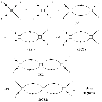
FIG. 1.: Perturbative diagrammatic expansion for the total vertex in terms of the bare interaction. At the two-loop level, only the diagrams employed in the Sec.IIID are depicted.

Let us define a flow parameter $t$ such that $\Lambda(t)=\Lambda_{0}e^{-t}$. We will follow the flow of the vertex function from $t=0$ to $t=\infty$. We introduce the dimensionless temperature $\beta_{R}(t)\equiv\frac{1}{2}v_{F}\beta\Lambda(t)$. Three Feynman diagrams contribute to the Gell-Mann–Low (GML) function of the vertex function at the one-loop level (see Fig. 1): zero sound (ZS), Peierls (ZS^′), and Cooper pairing (BCS). The coupling functions $\hat{\Phi}$ and ${\hat{V}}$ can be extracted from the vertex ${\hat{\Gamma}}$ by proper choice of the external momenta lying on the Fermi surface and by putting the external frequencies equal to the minimal Matsubara frequency $\omega_{min}\equiv\pi T$. Summations over flavor indices and Matsubara frequencies can be done easily using Eq. (II) and standard techniques[5, 14] for working with temperature Green’s functions. The relevant contributions to the GML functions of $\hat{\Phi}$ and $\hat{V}$ come only from those diagrams in which all the momentum phase space is available for integration. For a detailed discussion of this last issue, see Ref. [11].

To our knowledge, Shankar was the first to argue[11] that the RG fixed point in the Landau channel yields the Landau $\hat{f}$-function of the Fermi liquid. At zero temperature, Shankar obtained an RG-invariant function $\Phi^{A}$ and identified it with the Landau function. Our finite-temperature analysis reveals a more subtle situation.

As is known from the Landau FL theory[4], there are two limits of the four-point vertex function with all four momenta lying on the Fermi surface, depending on the way the limit of zero momentum- and energy-transfer is taken. One of these limits, which does not possess the symmetry (51) of the forward scattering amplitude , yields the Landau function. The other one, which preserves the antisymmetry of the vertex, gives the total forward scattering amplitude. For details see, for instance, the especially elucidative paper by Mermin.[18]

To clarify this point in our approach, let us consider the perturbative contribution of the ZS diagram to the vertex function ${\hat{\Gamma}}({\bf 1},{\bf 2};{\bf 3},{\bf 4})$ at small momentum transfer ${\bf q}={\bf K}_{3}-{\bf K}_{1}$ and small energy transfer $i\Omega_{13}=i(\omega_{1}-\omega_{3})$. As discussed after Eq. (35), we neglect the difference ${\bf K}^{i}-{\bf K}^{i}_{F}$ in the effective interaction. For this contribution we have:

$${\hat{\cal I}}_{ZS}({\bf K}_{F}^{1},{\bf K}_{F}^{2},{\bf q},\Omega_{13})=\int{d{\bf K}\over(2\pi)^{d}}U^{\alpha\mu}_{\gamma\nu}({\bf K}_{F}^{1},{\bf K}_{F};{\bf K}_{F}^{1},{\bf K}_{F})$$ (54)

$$\quad\times U^{\nu\beta}_{\mu\delta}({\bf K}_{F},{\bf K}_{F}^{2};{\bf K}_{F},{\bf K}_{F}^{2})L_{ZS}({\bf K},{\bf q},\Omega_{13})$$

where

$$L_{ZS}({\bf K},{\bf q},\Omega_{13})=\frac{1}{2}{\sinh(\beta v_{F}{\bf K}\cdot{\bf q}/2K_{F})\over i\Omega_{13}-v_{F}{\bf K}\cdot{\bf q}/K_{F}}$$ (55)

$$\quad\times\cosh^{-1}\left[\frac{1}{2}\beta v_{F}k\right]\cosh^{-1}\left[{\beta v_{F}\over 2K_{F}}{\bf K}_{F}\cdot({\bf k}+{\bf q})\right]$$ (56)

is the result of the summation of the product of two Green’s functions over Matsubara frequencies inside the loop. As follows from Eq. (55), $L_{ZS}$ has two limits: In the ‘unphysical’ limit (${\bf q}\to 0$, followed by $\Omega_{13}=0$) $L_{ZS}$ vanishes. In the ‘physical’ limit ($\Omega_{13}=0$, followed by ${\bf q}\to 0$), $L_{ZS}=-\frac{1}{4}\beta\cosh^{-2}(\frac{1}{2}\beta v_{F}k)$.

All the phase space is available for integration in the r.h.s. of Eq. (54), so the ZS diagram gives a relevant contribution to the total vertex at any angle $\theta$ between ${\bf K}_{F}^{1}$ and ${\bf K}_{F}^{2}$. A similar analysis for the ZS^′ diagram shows, that because of the phase space restrictions, it is relevant only when $\theta\to 0$, and its contribution does not depend on the way how zero energy- and momentum-transfer limit is taken:

$$\lim_{\theta\to 0}~{}{\hat{\cal I}}_{ZS^{\prime}}(0,0)=\int{d{\bf K}\over(2\pi)^{d}}U^{\alpha\mu}_{\delta\nu}({\bf K}_{F}^{1},{\bf K}_{F};{\bf K}_{F}^{1},{\bf K}_{F})$$ (57)

$$\quad\times U^{\nu\beta}_{\mu\gamma}({\bf K}_{F},{\bf K}_{F}^{1};{\bf K}_{F},{\bf K}_{F}^{1})\frac{1}{4}\beta\cosh^{-2}(\frac{1}{2}\beta v_{F}k)$$ (58)

In the following we will call $\hat{\Phi}(\theta,t)$ the renormalized dimensionless vertex in the ‘unphysical’ limit, i.e.

$$\hat{\Phi}(\theta,t)\equiv\frac{1}{2}\nu_{F}\left[\lim_{{\bf q}\to 0}{\hat{\Gamma}}({\bf 1},{\bf 2};{\bf 3},{\bf 4})\right]_{\Omega_{13}=0}$$ (59)

This notation is justified since the vertex function coincides with the effective interaction $\hat{\Phi}$ in that limit. On the other hand, we define the renormalized dimensionless vertex in the ‘physical’ limit as

$${\hat{\Gamma}}(\theta,t)\equiv\frac{1}{2}\nu_{F}\lim_{{\bf q}\to 0}\left[{\hat{\Gamma}}({\bf 1},{\bf 2};{\bf 3},{\bf 4})\bigg{|}_{\Omega_{13}=0}\right]$$ (60)

We will use the components of the vertex $\Gamma^{A,S}$ defined in the same fashion as in Eq. (25).

Note that among one-loop contributions to the GML function of the vertex $\hat{\Gamma}$ with arbitrary incoming and outgoing external momenta and frequencies, the BCS channel possesses the total symmetry of the interaction (Eqs. (25)), while the ZS (or ZS^′) channel separately do not: only their combined contribution is antisymmetric under exchange of incoming (or outgoing) particles. Here, the diagram ZS^′ contributes to the GML function of $\hat{\Phi}(\theta,t)$ when $\theta\to 0$, and it generates the flow for $\Phi^{A}(\theta,t)$ at $\theta=0$, breaking the condition $\Phi^{A}(0)=0$, while this ZS^′ contribution for the physical vertex cancels $\partial\Gamma^{A}(\theta,t)/\partial t$ at $\theta=0$. This makes the derivatives $\partial\Phi^{A}(\theta,t)/\partial t$ and $\partial\Gamma^{A}(\theta,t)/\partial t$ discontinuous at $\theta=0$. In reality, this feature is smeared over some angle $\theta_{sm}\sim\Lambda_{0}/K_{F}$, which is small ($\theta_{sm}\ll 1$) because of the condition (29). In order to obtain a smooth GML functions for $\hat{\Phi}(\theta,t)$ and $\hat{\Gamma}(\theta,t)$, we adopt the following procedure: First, we define $\hat{\Phi}(\theta,t)$ and $\hat{\Gamma}(\theta,t)$ in the patch $\theta\in[\theta_{0},\pi)$, where $\theta_{sm}<\theta_{0}\ll 1$. Then we derive the RG equations in this domain, and finally we analytically continue $\hat{\Phi}(\theta,t)$ and $\hat{\Gamma}(\theta,t)$ up to $\theta_{0}=0$.

The calculations are straightforward, and we end up with the following RG equations:

$${\partial\Phi^{A,S}_{l}\over\partial t}=0$$ (62)

$${\partial\Gamma^{A,S}_{l}\over\partial t}={\beta_{R}\over\cosh^{2}\beta_{R}}P^{A,S}_{l}$$ (63)

$${\partial\beta_{R}\over\partial t}=-\beta_{R}$$ (64)

Here we introduced the following notation:

$$P^{A}_{l} \equiv ~{}~{}{N+3\over 2}[\Gamma^{A}_{l}]^{2}-(N-1)\Gamma^{A}_{l}\Gamma^{S}_{l}+{N-1\over 2}[\Gamma^{S}_{l}]^{2}$$ (66)

$$P^{S}_{l} \equiv -{N+1\over 2}[\Gamma^{A}_{l}]^{2}+(N+1)\Gamma^{A}_{l}\Gamma^{S}_{l}-{N-3\over 2}[\Gamma^{S}_{l}]^{2}$$ (67)

As follows from Eqs. (1a), the functions $\Phi^{A,S}(\theta,t)$ are RG invariant. The effect of the singular contribution to the RG flow from the ZS^′ diagram is not included in Eq. (1a), but is equivalent to relaxing the symmetry condition $\Phi^{A}(0)=0$ for the bare coupling function $\Phi^{A}(\theta)$. It is convenient to express the RG invariants $\Phi^{A,S}$ in terms of ‘charge’ ($F$) and ‘flavor’ ($G$) functions, defined as follows:

$$F \equiv (N-1)\Phi^{S}-(N+1)\Phi^{A}$$ (69)

$$G \equiv -\Phi^{S}-\Phi^{A}$$ (70)

The physical meaning of these functions becomes clear in the case of real electron spin ($N=2$), when they coincide with the components of the Landau $\hat{f}$-function[13]:

$$f_{12,34}(\theta)=F^{(L)}(\theta)\delta_{13}\delta_{24}+G^{(L)}(\theta)\mbox{\boldmath$\sigma$}_{13}\cdot\mbox{\boldmath$\sigma$}_{24}$$ (71)

In order to decouple the Eqs. (1b) we introduce new components of the renormalized vertex ${\hat{\Gamma}}$:

$$A \equiv (N-1)\Gamma^{S}-(N+1)\Gamma^{A}$$ (73)

$$B \equiv -\Gamma^{S}-\Gamma^{A}$$ (74)

Their RG fixed points in the case $N=2$ coincide with the components of the total scattering amplitude in the notations of FL theory.[13] (Notice, that the components $\Gamma^{S}$ and $-\Gamma^{A}$ are respectively called singlet and triplet amplitudes in Ref. [19]). Notice also the symmetries $A_{l}=A_{-l}$ and $B_{l}=B_{-l}$. To simplify the system of Eqs. (1b) and (1c) we use an auxiliary RG parameter

$$\tau\equiv\tanh\beta_{R}~{},~{}~{}~{}\tau\in[0,\tau_{0}]$$ (75)

wherein $\tau_{0}\equiv\tanh\beta_{0}\leq 1$, and $\beta_{0}\equiv\frac{1}{2}v_{F}\beta\Lambda_{0}$.

Expressed in terms of these new variables, the RG equations become much simpler:

$${\partial A_{l}\over\partial\tau} = A_{l}^{2}$$ (77)

$${\partial B_{l}\over\partial\tau} = B_{l}^{2}$$ (78)

From Eqs. (1) we obtain the following stable fixed points (i.e. the solutions at $t=\infty$) :

$$A_{l}^{\ast} = {F_{l}\over 1+F_{l}\tau_{0}}$$ (80)

$$B_{l}^{\ast} = {G_{l}\over 1+G_{l}\tau_{0}}$$ (81)

where we expressed the bare values of the vertex via parameters of the effective interaction (the FL parameters), i.e. $A_{l}^{(0)}=F_{l}$, $B_{l}^{(0)}=G_{l}$. (In this work asterisks and zeros respectively denote fixed points and bare values.) From Eq. (III B) it follows that, if the parameters of interaction satisfy the conditions

$$\{F_{l},G_{l}\}>-1~{},\qquad\forall~{}l$$ (82)

the system will remain stable in the Landau channel at any temperature. The fixed point (III B) at $T=0$ ($\tau_{0}=1$) gives the same solution for the forward scattering vertex as the Bethe-Salpeter equation in the zero-temperature technique.[5, 13] Notice that, because of the condition $T\ll v_{F}\Lambda_{0}$ imposed on the low-energy effective action, we can set $\tau_{0}=1$ for all practical purposes. Any attempt to extract a critical temperature from Eq. III B by looking at the violation of condition (82) for the absence of poles in the vertex function, would involve exponentially small corrections to zero temperature, thus exceeding the accuracy of the present approach.

To take into account the RG flow from the ZS^′ diagram, which preserves the symmetry condition $\Gamma^{A}(\theta=0,t=\infty)=0$, we impose the constraint

$$\sum_{l=-\infty}^{\infty}\left((N-1)A_{l}^{\ast}+B_{l}^{\ast}\right)=0$$ (83)

on the fixed point of the vertex. This specific form (83) of the condition for the forward scattering amplitudes is usually called the amplitude sum rule in FL theory.[5, 13]

C The RG equations in the BCS channel

The only relevant contribution to the GML function for $\hat{V}(\theta,t)$ comes from the BCS diagram. The fact that the BCS diagram preserves by itself the symmetry (III A) of the function $\hat{V}$ makes life simpler. The RG equations are derived easily:

$${\partial V^{A}_{l}\over\partial t} ~{}=~{} \phantom{-}\tanh\beta_{R}~{}(V^{A}_{l})^{2}\qquad\hbox{($l$ odd)}$$ (85)

$${\partial V^{S}_{l}\over\partial t} ~{}=~{} -\tanh\beta_{R}~{}(V^{S}_{l})^{2}\qquad\hbox{($l$ even)}$$ (86)

At zero temperature, Eq. (III Ca) coincides with Shankar’s result[11] for spinless fermions.[1]

The RG equations (III C) may be solved easily, and their fixed points are:

$$V^{A(\ast)}_{l} = {V^{A(0)}_{l}\over 1-V^{A(0)}_{l}\int_{0}^{\infty}\tanh(\beta_{0}e^{-t})dt}$$ (88)

$$V^{S(\ast)}_{l} = {V^{S(0)}_{l}\over 1+V^{S(0)}_{l}\int_{0}^{\infty}\tanh(\beta_{0}e^{-t})dt}$$ (89)

The system remains stable in the $\hat{V}$ channel at any temperature if, for all harmonics, the following conditions are fulfilled:

$$V^{A(0)}_{l} < 0$$ (91)

$$V^{S(0)}_{l} > 0$$ (92)

At low temperature (i.e., when the low-energy action approach is supposed to work well), $\beta_{0}\gg 1$ and the integrals of Eqs. (III C) can be evaluated exactly, like in the theory of superconductivity (cf. section 33.3 of Ref. [5]):

$$V^{A(\ast)}_{l} = {V^{A(0)}_{l}\over 1-V^{A(0)}_{l}\ln(2\tilde{\gamma}v_{F}\Lambda_{0}/\pi T)}$$ (94)

$$V^{S(\ast)}_{l} = {V^{S(0)}_{l}\over 1+V^{S(0)}_{l}\ln(2\tilde{\gamma}v_{F}\Lambda_{0}/\pi T)}$$ (95)

wherein $\ln\tilde{\gamma}\equiv\gamma\approx 0.577$ is Euler’s constant. If the conditions (III C) are violated, the $\hat{V}$-interaction becomes marginally relevant, and a pole appears at temperature

$$T^{(l)}_{SC}={2\tilde{\gamma}\over\pi}v_{F}\Lambda_{0}\exp(-{1\over\Xi_{l}})$$ (96)

Here $\Xi_{l}\equiv max\{V^{A(0)}_{l},|V^{S(0)}_{l}|\}$, in which only the harmonics violating the condition (III C) are included. If phonons provide the underlying mechanism of attraction, we may identify the characteristic energy scale $v_{F}\Lambda_{0}$ of the low-energy action with the Debye energy $\omega_{D}$. In the present context, the BCS theory of superconductivity corresponds to the special case of a contact attractive interaction, for which only the zeroth harmonic $V^{S(0)}_{0}\propto U_{0}<0$ does not vanish.

D Beyond the one-loop approximation

The main goal of this subsection is to argue that there are no higher-loop corrections neither into one-particle Green’s function, nor into the vertex. In other words, the one-loop RG results are exact for this model, based on the low-energy effective action.[11]

The phase space analysis of the diagrams contributing to the self-energy $\Sigma$ shows, that the only relevant contribution comes from the tadpole diagram at the one-loop level, and diagrams obtained from it by tadpole self-energy insertions at higher loops. This self-energy contribution is temperature-independent, and it results in a mere shift of chemical potential of the interacting system $\mu_{int}$. As far as we retain the constant density of particles in the system, the self-energy contribution exactly compensates the change of the chemical potential due to interaction at $T=0$, i.e. $\mu_{int}(T=0)-\Sigma=\mu=K_{F}^{2}/m^{\ast}$, according to the Luttinger theorem.[20] So, the renormalization of the one-particle Green’s function due to the self-energy holds its linearized form (32) near the Fermi surface unchanged. It supposes also the temperatures under consideration being small enough to neglect the temperature corrections to the chemical potential of the interacting system.

Thus, integration over the rest of the degrees of freedom inside the narrow shell around the Fermi surface neither generates an additional wavefunction renormalization (we have chosen the initial scale of the Grassmann fields in the bare effective action such that $Z=1$), nor an additional renormalization of the effective mass of quasiparticles (i.e. the phenomenological parameter of the effective action $v_{F}=K_{F}/m^{\ast}$ does not change).

To show that the RG results obtained above are exact for this model, we will demonstrate the cancellation of the next terms in the GML functions at the two-loop level. The generalization of this proof to higher loops is straightforward. In this subsection we use the standard field-theory renormalization technique[21, 22] with momentum integrations taken over the interval $k\in[-\Lambda,\Lambda]$, instead of the Wilson-Kadanoff (WK) scheme. Since we work at finite temperature, there is no need to introduce an infrared cutoff, because all integrals are regular near the point $k=0$. The pictorial form of the equation for the renormalized vertex in terms of the 1PI-diagrams is presented in Fig. 1. The light squares stand for the bare vertices, while the dark square denotes the renormalized vertex. The equation for the renormalized vertex may be written in the symbolic short-hand form as:

$$u_{R}=u_{0}-u_{0}^{2}L_{1}+u_{0}^{3}L_{2}$$ (97)

From Eq. (97) the GML function $\beta_{GML}=(\partial u_{R}/\partial\ln\Lambda)_{u_{0}}$ is found to be

$$\beta_{GML}(u_{R})=-u_{R}^{2}L_{1}^{\prime}+u_{R}^{3}(L_{2}-L_{1}^{2})^{\prime}$$ (98)

where the primes in the r.h.s. of Eq. (98) stand for the partial derivative w.r.t. $\ln\Lambda$. We can use symbolic form (98) for the calculation of the GML functions for renormalized functions $\hat{\Phi}(\theta,\Lambda)$, ${\hat{\Gamma}}(\theta,\Lambda)$, and ${\hat{V}}(\theta,\Lambda)$.

The phase space analysis of the two-loop diagrams shows that the only relevant contribution to $L_{2}$ in the Landau channel comes from the diagram $ZS2$. In the unphysical limit this contribution is zero, while in the physical limit it is exactly canceled by the term $-L_{1}^{2}$ which in this case is the contribution from the one-loop ZS diagram. Therefore, Eqs. (1a, b) are true at two-loop level as well. In the BCS channel, the only relevant contribution to $L_{2}$ in the equation for the GML function of ${\hat{V}}(\theta,\Lambda)$ comes from the diagram BCS2, and in the same way it is canceled by the contribution $L_{1}$ from the BCS diagram, leaving Eq. (III C) unchanged.

It is worth noticing that the above proof of the cancellation of higher-order terms of the GML functions do not work in one dimension, because the phase space restrictions in 1D are not strong enough to remove the contributions from all higher-loop diagrams. At the two-loop level, the term $L_{2}$ in Eq. (98) includes the contributions from all 1PI vertex diagrams along with the self-energy ‘sunrise’ diagram contribution, responsible for the wavefunction renormalization. Thus, in 1D there is no cancellation in the GML functions due to renormalization.

IV The RG equations in three dimensions

In order to obtain the marginal coupling functions for a spherical Fermi surface in 3D, we follow the same procedure as in Sec.III. There are two marginal coupling functions:

1. The function $\hat{\Phi}$.  It is defined by Eq. (36). It couples a pair of fermions with momenta $({\bf K}^{1}_{F},{\bf K}^{2}_{F})$ to another pair with momenta $({\bf K}^{3}_{F},{\bf K}^{4}_{F})$, lying on the cone swept by a rotation of $({\bf K}^{1}_{F},{\bf K}^{2}_{F})$ around the vector ${\bf K}^{1}_{F}+{\bf K}^{2}_{F}$. Let $\theta_{12}$ be the angle between two vectors ${\bf K}^{1}_{F}$ and ${\bf K}^{2}_{F}$, and $\phi_{13}$ the angle between the two planes defined by the pairs $({\bf K}^{1}_{F},{\bf K}^{2}_{F})$ and $({\bf K}^{3}_{F},{\bf K}^{4}_{F})$. The function $\hat{\Phi}$ may be written as

$$\hat{\Phi}=\Phi^{A}(\theta_{12},\phi_{13})I^{\alpha\beta}_{\gamma\delta}+\Phi^{S}(\theta_{12},\phi_{13})T^{\alpha\beta}_{\gamma\delta}$$ (99)

wherein the functions $\Phi^{A,S}$ have the following symmetry properties:

$$\Phi^{A}(\theta_{12},\phi_{13}\pm\pi) = -\Phi^{A}(\theta_{12},\phi_{13})$$ (101)

$$\Phi^{S}(\theta_{12},\phi_{13}\pm\pi) = ~{}~{}\Phi^{S}(\theta_{12},\phi_{13})$$ (102)

The minimal domain of definition allowing to recover all values of these functions is $\theta,\phi\in[0,\pi)$.

2. The function $\hat{V}$.  It is defined by Eq. (III Aa), with the symmetry properties (III A).

The phase space analysis shows that the RG flow is generated only in the forward scattering amplitude channel, i.e., in the ‘physical’ limit of the vertex ${\hat{\Gamma}}(\theta)$. All other coupling functions are RG invariant and never mix up with the $\phi=0$ channel. Like in the 2D case, the relevant contributions to the GML functions of ${\hat{\Gamma}}(\theta,t)$ and $\hat{V}(\theta,t)$ come respectively from the diagrams ZS and BCS.

The spherical symmetry of the Fermi surface makes convenient an expansion of these functions into Legendre polynomials. Using again the short-hand notation X for the set of coupling functions (cf Eq. (III A)), this expansion is

$${\bf X}(\theta) = \sum_{l=0}^{\infty}~{}(2l+1)~{}{\bf X}_{l}~{}P_{l}(\cos\theta)$$ (104)

$${\bf X}_{l} = \frac{1}{2}\int_{-1}^{1}d(\cos\theta)~{}{\bf X}(\theta)~{}P_{l}(\cos\theta)$$ (105)

Here, in the set ${\bf X}(\theta)$, $\Phi^{A,S}(\theta)$ stands for $\Phi^{A,S}(\theta,\phi=0)$. All the calculations are conducted in the same way as in the previous section.

The symmetry properties and the RG equations of $\hat{V}$ are exactly the same as in two dimensions. The only technical modification in the Landau channel is the sum rule for partial amplitudes (cf. Eq. (83))

$$\sum_{l=0}^{\infty}(2l+1)\left[(N-1)A_{l}^{\ast}+B_{l}^{\ast}\right]=0$$ (106)

The rest of the formulas and all the conclusions made in the 2D case may be repeated word for word in the 3D case.

V Response functions

In this section we apply our RG technique to the study of response functions. (For the definitions of these functions and their relationship with physical observables, see, for instance, Ref. [14].) All the results presented below are valid for spatial dimensions $d=2,3$. In order to calculate the compressibility, we consider the density response function $\kappa({\bf Q})$, defined as follows:

$$\delta^{(d+1)}(0)\kappa({\bf Q})\equiv\langle\tilde{\rho}({\bf Q})\tilde{\rho}^{{\dagger}}({\bf Q})\rangle$$ (107)

wherein the density operator $\rho({\bf Q})$ is

$$\rho({\bf Q})=\int_{({\bf 1})}\bar{\psi}_{\alpha}({\bf 1})\psi_{\alpha}({\bf 1}+{\bf Q})$$ (108)

and $\tilde{\rho}({\bf Q})=\rho({\bf Q})-\langle\rho({\bf Q})\rangle$ stands for the density fluctuation. Here ${\bf Q}\equiv({\bf q},\Omega_{n})$, and $\Omega_{n}$ is the Matsubara frequency. The zeroth component of this function $\kappa({\bf Q})$ taken in the physical limit gives us the derivative of the particle concentration $n$ w.r.t. the chemical potential, i.e.

$$\kappa\equiv\lim_{{\bf q}\to 0}\left[\kappa({\bf Q})\bigg{|}_{\Omega_{n}=0}\right]={\partial n\over\partial\mu}$$ (109)

The RG flow is simplest when obtained in the field-theory renormalization scheme, like in the Sec. IIID. Notice, that in this scheme the RG parameter $\tau$ (cf. Eq. (75)) runs from $\tau=0$ to $\tau=\tau_{0}\approx 1$ (the fixed point), and the r.h.s. of Eqs. (1) changes its sign. The first two terms of the perturbative expansion for $\kappa$ give us (cf. Eq. (1))

$$\kappa\simeq\kappa_{0}-\kappa_{0}\tau A_{0}^{(0)}$$ (110)

wherein $\kappa_{0}={N\over 2}\nu_{F}\tau$ is the contribution from the free part of the effective action. According to the results of the Sec. IIID, to obtain the equation for the RG flow of $\kappa(\tau)$, exact in this model, it is sufficient to take into account one-loop renormalization of the physical vertex. Introducing the auxiliary function $\bar{\kappa}(\tau)\equiv\kappa/\kappa_{0}$, and using Eqs. (1), we get the RG equation:

$${\partial\ln\bar{\kappa}(\tau)\over\partial\tau}=-A_{0}(\tau)$$ (111)

which yields $\partial n/\partial\mu$ as its fixed point:

$$\kappa^{\ast}={N\over 2}{\nu_{F}\over 1+F_{0}}$$ (112)

From the thermodynamic formula for the compressibility $K\equiv-(1/V)(\partial V/\partial P)=(1/n^{2})(\partial n/\partial\mu)$ (see, for instance, Ref. [19]), we easily recover the result for the electron Fermi liquid:

$$K={1\over n^{2}}{\nu_{F}\over 1+F_{0}}$$ (113)

To find the spin susceptibility in our $SU(N)$ formalism, we consider the flavor response function $\chi({\bf Q})$, defined as follows

$$\delta^{(d+1)}(0)\chi({\bf Q})\equiv{1\over N^{2}-1}\langle S_{a}({\bf Q})S_{a}^{{\dagger}}({\bf Q})\rangle$$ (114)

wherein the flavor density operator

$$S_{a}({\bf Q})={g\over 2}\int_{({\bf 1})}\lambda^{a}_{\alpha\beta}\bar{\psi}_{\alpha}({\bf 1})\psi_{\beta}({\bf 1}+{\bf Q})$$ (115)

and $g$ is the gyromagnetic ratio. The uniform susceptibility $\chi$ is given by the physical limit $\chi({\bf Q}\to 0)$ (cf. Eq. (109)). Defining $\chi({\bf Q})$ in the fashion (114), we used the fact that in the paramagnetic state the response is the same along all the $(N^{2}-1)$ directions $a$. The rest of the calculations is carried out in the same way as above. For the auxiliary function $\bar{\chi}(\tau)\equiv\chi/\chi_{0}$ ($\chi_{0}=\frac{1}{4}g^{2}\nu_{F}\tau$ is the contribution in the absence of interaction) we obtain the RG equation:

$${\partial\ln\bar{\chi}(\tau)\over\partial\tau}=-B_{0}(\tau)$$ (116)

Again, we recover the FL theory result:[19]

$$\chi^{\ast}=\frac{1}{4}g^{2}{\nu_{F}\over 1+G_{0}}$$ (117)

Notice, that the stability conditions for the fixed points (112) and (117) are just a special case ($l=0$) of the general conditions (82).

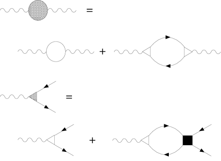
FIG. 2.: Diagrammatic form of the recursion relations for the susceptibility $\chi(t)$ (circle) and the vertex $z(t)$ (triangle). The hatched symbols stand for the functions at $t+dt$, whereas light ones stand for functions at $t$. The black square stands for the vertex $\hat{\Gamma}(t)$. Integration over loop momenta is carried out in an infinitesimal shell $d\Lambda(t)$.

It is interesting to show how the results (112) and (117) can be obtained in the Wilson-Kadanoff scheme.[2] Below we specialize to the electron ($N=2$) spin susceptibility, but the compressibility may be computed in the same fashion. We add to the effective action a source field $h({\bf Q})$, conjugated to the $z$-component of the spin density (115). For details on this approach, see, for instance, Ref. [7]. The successive integration over momentum modes generates a vertex correction $z(t)$ to the source term along with higher order terms in the external field $h$. The effective action, at some intermediate value of $t$ (the flow parameter), takes the form

$$S[\psi,h,t] = S[\psi,0,t]+\int_{({\bf Q})}z(t,{\bf Q})\left[h({\bf Q})S_{3}({\bf Q},t)+h.c.\right]$$ (119)

$$~{}+~{}\int_{({\bf Q})}\chi(t,{\bf Q})h^{*}({\bf Q})h({-\bf Q})~{}+~{}{\cal O}(h^{3})$$

In linear response theory it is sufficient to keep track of terms up to second order in $h$. The recursion relations for the vertex $z(t)$ and the susceptibility $\chi(t)$ are illustrated on Fig. 2. In the physical limit ${\bf Q}\to 0$, we obtain the following pair of RG equations:

$${\partial\chi\over\partial\tau}=-\frac{1}{4}g^{2}\nu_{F}z^{2}(\tau)\qquad\qquad{\partial z\over\partial\tau}=z(\tau)B_{0}(\tau)$$ (120)

with the initial conditions $z(\tau_{0})=1$ and $\chi(\tau_{0})=0$. Using the solution for $B_{0}(\tau)$ which follows from (1b), we can easily solve this system. The uniform susceptibility, which is the fixed point of these equations, is again given by Eq. (117). Notice that one cannot simply compute the susceptibility (or any other response function) from the usual diagrammatic expression at the fixed point action: one would obtain zero at any non-zero temperature.

In order to obtain the heat capacity in this model, one does not need to perform any complicated calculation. As explained in Sec. IIID, tracing over fermion modes in the vicinity of the Fermi surface in $d=2$ and 3 does not modify the one-particle Green’s function (32). Therefore, the only relevant part of the free energy expressed as a functional of the total Green’s function[20] is the same as for the effective action (2) without the interacting part. It simply gives the Fermi liquid result $C=\frac{1}{6}\pi^{2}N\nu_{F}T$.

VI Conclusion

The RG approach to interacting fermions has been extended to the case of non-zero temperature and spin. We studied a model with $SU(N)$-invariant short-range effective interaction and rotationally invariant Fermi surface. In general, the RG approach turns out to be equivalent to Landau’s mean-field treatment of the Fermi liquid. The first set of conditions (III C) for the bare couplings of the low-energy action is nothing but Landau’s theorem for the stability of Fermi liquids against Cooper pairing at arbitrary angular momentum.[13] Likewise, conditions (82) for the system to be stable up to zero temperature are Pomeranchuk’s conditions for the components of the Landau interaction function. Only if both conditions (III C) and (82) are fulfilled does the system reach zero temperature in the Fermi liquid regime. One advantage of the finite-temperature formalism is to reveal the possible breakdown of the FL picture below some critical temperature $T_{c}$, whereas it remains applicable above $T_{c}$.

The distinction between physical and unphysical limits as momentum and frequency go to zero appears naturally in this finite temperature formalism, and differentiates the Landau function from the scattering vertex. The former is RG invariant, whereas the latter flows towards a fixed point (III B), which reproduces the well-known relationship between components of the Landau function and the forward scattering amplitudes. Working in the finite-temperature formalism made explicit the equivalence of the results obtained in the Wilson-Kadanoff and field-theory schemes of renormalization. Notice that, in the Wilson-Kadanoff scheme at zero temperature, the RG flow of the physical scattering vertex might be easily overlooked,[11] since special care must be taken when the shrinking cut-off crosses the scale given by non-zero transferred momentum.

In general, temperature plays the role of a ‘natural regulator’ in this theory. Firstly, it eliminates the need for an infrared cut-off in the BCS channel. Secondly, and more important, it makes the Gell-Mann–Low functions smooth in the Landau channel.[3] Thus, the fixed points are smooth functions in the $T\to 0$ limit.

Response functions, like the spin susceptibility or the compressibility, are naturally defined in the physical limit, and thus their RG flow involves the physical vertex $\hat{\Gamma}(t)$, which then plays the role of a ‘running’ effective interaction. This makes superfluous the use of any additional perturbative calculation[11] once the fixed point is reached.

- [1] The reader might be slightly confused by the sign of the r.h.s. of Eq. (III Ca) when comparing our result with that of Shankar for the spinless Hubbard model. In fact, this sign is just a consequence of the way we define the coupling function in this work. Indeed, let us consider the Hubbard Hamiltonian on a -dimensional hypercubic lattice (with lattice constant ) at low filling, with on-site () and nearest-neighbor () interactions. Both constants are positive for a repulsive interaction, and negative for attraction. Fourier-transforming and symmetrizing the interaction, we end up with the following coupling functions of the microscopic Hamiltonian: and . Here, only the lowest order terms in the expansion of trigonometric functions were kept. Then we can use this result as the lowest-order approximation for the bare coupling functions of in the definitions (36) and (III A).
- [2] For the following discussion we are indebted in great part to N. Dupuis.
- [3] Notice that, in Eq. (1b), .
- [4] L.D. Landau, Soviet Phys.-JETP 8, 70 (1959).
- [5] A.A. Abrikosov, L.P. Gorkov, and I.E. Dzyaloshinski, Methods of Quantum Field Theory in Statistical Physics (Dover, New York, 1963).
- [6] J. Solyom, Adv. Phys. 28, 201 (1979).
- [7] C. Bourbonnais, L.G. Caron, Int. J. Mod. Phys. B5, 1033 (1991).
- [8] G. Benfatto and G. Gallavotti, J. Stat. Phys. 59, 541 (1990);Phys. Rev. B42, 9967 (1990).
- [9] R. Shankar, Physica A 177, 530 (1991).
- [10] J. Polchinski, in Proceedings of the 1992 Theoretical Advanced Studies Institute in Elementary Particle Physics, ed. J. Harvey and J. Polchinski (World Scientific, Singapore, 1993).
- [11] R. Shankar, Rev. Mod. Phys. 66, 129 (1994).
- [12] S. Weinberg, Nucl. Phys. B413 [FS], 567 (1994).
- [13] E.M. Lifshitz and L.P. Pitayevskii, Statistical Physics II (Pergamon Press, Oxford, 1980).
- [14] J.W. Negele and H. Orland, Quantum Many-Particle Systems (Addison-Wesley, New York, 1988).
- [15] T.-P. Cheng and L.-F. Li, Gauge Theory of Elementary Particle Physics (Oxford University Press, New York, 1984).
- [16] J.P. Elliot and P.G. Dawber, Symmetry in Physics, v.1,2 (The Macmillan Press Ltd, London, 1979).
- [17] A. Houghton, H.-J. Kwon, and J.B. Marston, Phys. Rev. B 50, 1351 (1994).
- [18] N.D. Mermin, Phys. Rev. 159, 161 (1967).
- [19] G. Baym and C. Pethick, Landau Fermi-Liquid Theory (John Wiley and Sons, New York, 1991).
- [20] J.M. Luttinger, Phys. Rev. 119, 1153 (1960).
- [21] E. Brézin, J.C. Le Guillou, and J. Zinn-Justin, in Phase Transitions and Critical Phenomena, v.6, eds. C. Domb and M.S. Green (Academic Press, New York, 1976).
- [22] D.J. Amit, Field Theory, the Renormalization Group, and Critical Phenomena (World Scientific, 1984).