cond-mat/9505076
Renormalization Group Analysis of a Noisy Kuramoto-Sivashinsky Equation

I Introduction

Currently, there is much interest in understanding the formation and roughening of nonequilibrium interfaces [2, 3, 4, 5, 6]. A common feature of many interfaces observed experimentally and in discrete models is that their roughening follows simple scaling laws characterized by the roughness exponent $\alpha$ and the dynamic exponent $z$, which determine the scaling behavior of, e.g., the correlation functions. In many cases, the scaling exponents can be obtained using stochastic evolution equations of which a seminal example is the so-called Kardar-Parisi-Zhang (KPZ) equation [7, 8].

Another equation, which has been actively discussed in problems of pattern formation, such as chemical turbulence and flame-front propagation, is the so-called Kuramoto-Sivashinsky (KS) equation [9, 10, 11, 12]. This is a deterministic nonlinear equation which exhibits spatiotemporal chaos. Qualitatively, the chaotic nature of the KS equation generates stochasticity in such a way that its solution displays scaling at large distances and long times. An important question to answer is whether the KPZ and KS equations belong to the same or to different universality classes, i.e., whether the scaling properties of the interfaces are described by the same or different values for the critical exponents. In $1+1$ dimension there are numerical [13, 14, 15, 16, 17] and analytical [17, 18, 19, 20] results which show that the KS and KPZ equations indeed exhibit the same scaling behavior. However, it is still an open question whether the KS and the KPZ equations fall into the same universality class in $2+1$ dimensions [19, 20, 21, 22].

In order to address these questions from a different point of view, we have investigated a noisy version of the KS equation by a dynamic renormalization group (RG) analysis. Even though the relation of such a noisy KS equation to the KS system is still to be completely clarified, we believe that the results we obtain for the scaling behavior of the noisy KS equation may be suggestive concerning the relation between the KS and KPZ equations in one and two spatial dimensions. Moreover, the noisy KS equation studied here may be relevant for the understanding of dynamic roughening in, e.g., sputter eroded surfaces and, in principle, to any physical system modeled by the deterministic KS equation in which the relevance of time dependent noise as, e.g., fluctuations in a flux or thermal fluctuations, can be argued for.

The outline of this paper is as follows. In the next section we introduce the noisy KS equation and discuss how it naturally arises in the description of ion-sputtering. Then we derive the RG flow in section III. Section IV contains the analysis of the RG flow and our results for one and two spatial dimensions. Finally, in section V we conclude and summarize.

II The Noisy Kuramoto-Sivashinsky Equation

In this section we introduce the noisy KS equation and address some of its peculiarities and limiting cases. We discuss a physical example in which the noisy KS equation appears naturally, namely surfaces eroded by ion-sputtering.

Recently, the dynamics of surfaces undergoing ion-sputtering have been studied experimentally and several different scaling behaviors found [23, 24, 25]. Among them it is noteworthy to remark the values $\alpha=0.2-0.4$, and $z=1.6-1.8$ [23], which are consistent with the predictions of the KPZ equation in $2+1$ dimensions [5, 6]. On the other hand, it is well known that for amorphous targets, ion-sputtering leads in many cases to the formation of a periodic ripple structure whose orientation depends on the angle of incidence, $\theta$, of the ions with the normal to the uneroded surface [26]. This periodic structure is associated with an instability in the system. An experimental study of this kind of morphologies can be found in [24]. In Ref. [27] a nonlinear stochastic equation has been proposed to describe the dynamics of the surface profile height $h(x,t)$ of a two-dimensional surface sputtered at off-normal angles. The $\theta\to 0$ limit (normal incidence) of this equation results in

$$\frac{\partial h}{\partial t}=\nu\nabla^{2}h-K(\nabla^{2})^{2}h+\frac{\lambda}{2}(\nabla h)^{2}+\eta(x,t).$$ (1)

Here, we will consider the case where the field $h(x,t)$ describes the height profile of a $d$-dimensional surface evolving in a $d+1$-dimensional medium. The surface tension coefficient $\nu$ is negative, whereas $K$ is a positive surface diffusion coefficient [28]. The strength of the nonlinearity is given by $\lambda$, and $\eta(x,t)$ is a Gaussian white noise with zero mean and short-range correlations described by

$$\langle\eta(x,t)\eta(x^{\prime},t^{\prime})\rangle=2D\delta^{d}(x-x^{\prime})\delta(t-t^{\prime}).$$ (2)

The fact that $\nu<0$ means that the system is linearly unstable, a fact which in ion-sputtered systems is related to faster erosion velocity at the bottom of the troughs than at the peaks of the crests [29], which in turn is related to the formation of the periodic ripple structure referred to above. The same kind of instability takes place in the deterministic KS equation, which corresponds to Eq. (1) without the noise term. In the following we will refer to Eq. (1) as the noisy KS equation. From a linear stability analysis one finds that the amplitude for solutions of the form

$$h_{0}(x,t)\sim\exp(\Omega_{k}t)\sin(kx)$$ (3)

is characterized by the rate $\Omega_{k}=-(\nu k^{2}+Kk^{4})$. This expression is plotted in Fig. 1, and seen to have a positive value (corresponding to unstable modes in the system) for momenta between $0$ and $k_{0}$, where

$$k_{0}=\sqrt{\frac{|\nu|}{K}}.$$ (4)

The modes with $k>k_{0}$ are stable. In this sense, $k_{0}$ marks the onset of the unstable modes, and the length scale $1/k_{0}$ can be related to the wavelength of the ripple structure. The nonlinearity $\lambda$ couples the stable and unstable modes, thus stabilizing the system [12]. If $\nu\geq 0$, it follows that all the modes in the noisy KS equation are stable and $k_{0}$ is not defined.

If $\nu$ in Eq. (1) is a positive coefficient, the contribution of the $K$ term is expected to be negligible at large length scales and for long times, so that in this case the noisy KS equation will show the same scaling behavior as the KPZ equation [7]

$$\frac{\partial h}{\partial t}=\nu\nabla^{2}h+\frac{\lambda}{2}(\nabla h)^{2}+\eta(x,t),$$ (5)

which is obtained as the $K=0$ limit of the noisy KS equation. However, if $\nu<0$ in Eq. (1), as is the case we are interested in, the surface diffusion term acts as a stabilizing mechanism at short length scales. In this situation it is not a priori clear what the scaling properties of Eq. (1) are.

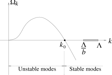
FIG. 1.: Stability of Fourier modes for the noisy KS equation. The modes from $0$ to $k_{0}$ are unstable, whereas those lying between $k_{0}$ and $\Lambda$ are stable, with $\Lambda$ the momentum cutoff. The shaded region corresponds to the momentum shell $\Lambda/b<k<\Lambda$ discussed in the text.

III RG Flow for the Noisy KS Equation

The renormalization group is a standard tool which can be applied to stochastic equations in order to determine their scaling behavior in the large-distance long-time hydrodynamic limit [30]. Basically, the RG consists of the combination of a coarse-graining of the system followed by rescaling by a factor $b=e^{\ell}$. Successive applications of this transformation leads to the RG flow of the parameters appearing in the equation in terms of the scale $\ell$. As usual, we will be interested in considering the variation of the parameters when $\ell$ is infinitesimal, that is, the flow is given by first order differential equations with respect to $\ell$. The critical exponents $\alpha$ and $z$ characterize the scaling behavior of, e.g., the correlation function

$$C(x-x^{\prime},t-t^{\prime}) = \left<\left[h(x,t)-h(x^{\prime},t^{\prime})\right]^{2}\right>$$ (6)

$$= |x-x^{\prime}|^{2\alpha}g\left(|t-t^{\prime}|/|x-x^{\prime}|^{z}\right),$$ (7)

where $g$ is a scaling function. These exponents are calculated at the fixed points of the RG transformation.

The standard implementation of the RG procedure to deal with equations such as Eq. (1) proceeds first by transforming it to Fourier space. In our case, it can be easily seen that the instability ($\nu<0$) in Eq. (1) generates a pole for zero frequency at the wavevector $k=k_{0}$ in the bare propagator

$$G_{0}(k,\omega)=\frac{1}{-i\omega+\nu k^{2}+Kk^{4}}.$$ (8)

As a result, when trying to solve the equation additional divergencies arise together with those existing for $k\to 0$. The RG circumvents these divergencies by integrating out a small momentum shell and can consistently be performed. The momentum shell corresponds to the wavevectors

$$\Lambda/b<k<\Lambda,$$ (9)

where the momentum cutoff $\Lambda\equiv 2\pi/a$ is related to the lattice spacing $a$, which acts as a short distance cutoff. Without loss of generality, we take $\Lambda\equiv 1$ in the following.

The existence of the $k_{0}$ pole splits the momentum axis in two regions where the coarse-graining procedure can be applied. The cutoff $\Lambda$ can either be put in the band of stable modes, cf. Fig. 1, or in the band of unstable modes. We will discuss the outcome of the RG analysis for both choices. Intuitively, however, one should coarse-grain over a shell of stable modes and study the effect of this coarse-graining on the large scales by means of the RG transformation.

The calculation of the complete RG flow for the noisy KS equation (1) is tedious. We follow standard diagrammatic procedures [8, 31] and here we only give the final result (see, e.g., [32]). Compared to the calculations for the KPZ equation ($K=0$) [7, 8, 31], the main source of the complications is that we have to keep terms up to order $k^{4}$ in our expansion, in order to be able to calculate the renormalization of the $-Kk^{4}$ term. The complete RG flow for the noisy KS equation at one-loop order is [33]

$$\frac{d\nu}{d\ell} = \nu\left(z-2+\frac{\lambda^{2}D}{\nu}K_{d}\,\frac{\nu(2-d)+K(4-d)}{4d(\nu+K)^{3}}\right)\!,$$ (10)

$$\frac{dK}{d\ell} = \!K\!\left(\!z-4+\frac{\lambda^{2}D}{K}K_{d}\right.$$ (13)

$$~{}~{}~{}~{}~{}~{}~{}~{}~{}~{}~{}\left.\times\frac{a_{0}\nu^{3}+a_{1}\nu^{2}K+a_{2}\nu K^{2}+a_{3}K^{3}}{16d(d+2)(\nu+K)^{5}}\right)\!\!,\!\!\!\!$$

$$\frac{d\lambda}{d\ell} = \lambda\left(\alpha+z-2\right)\!,$$ (15)

$$\frac{dD}{d\ell} = D\left(z-2\alpha-d+\lambda^{2}DK_{d}\,\frac{1}{4(\nu+K)^{3}}\right)\!,$$ (17)

with $K_{d}=S_{d}/(2\pi)^{d}$, where $S_{d}=2\pi^{d/2}/\Gamma(d/2)$ is the surface area of the $d$ dimensional unit sphere. The polynomials $a_{i}=a_{i}(d)$ ($i=0,1,2,3$) are given by

$$a_{0} = 3d(d-2),~{}~{}~{}~{}~{}~{}~{}~{}~{}~{}~{}~{}~{}\!a_{1}=11d^{2}-24d-20,$$ (18)

$$a_{2} = 13d^{2}-40d-60,~{}~{}~{}~{}a_{3}=5d^{2}-22d-16.$$ (19)

When studying the above RG flow, the coupling constants are conveniently taken to be

$$g_{\nu}=\frac{K_{d}}{4d}\frac{\lambda^{2}D}{\nu^{3}},\mbox{~{}~{}~{}~{}~{}~{}}f_{\nu}=\frac{K}{\nu}.$$ (20)

Using these variables, the flow (10)$-$(17) reads

$$\frac{dg_{\nu}}{d\ell} = (2-d)g_{\nu}+{4d-6+3(d-4)f_{\nu}\over(1+f_{\nu})^{3}}g_{\nu}^{2},$$ (21)

$$\frac{df_{\nu}}{d\ell} = -2f_{\nu}+{b_{0}+b_{1}f_{\nu}+b_{2}f_{\nu}^{2}+b_{3}f_{\nu}^{3}+b_{4}f_{\nu}^{4}\over 4(d+2){(1+f_{\nu})^{5}}}g_{\nu}.$$ (23)

The polynomials $b_{i}=b_{i}(d)$ ($i=0,1,\ldots,4$) are given by

$$b_{0} = 3d^{2}-6d,~{}~{}~{}~{}~{}~{}~{}~{}~{}~{}~{}~{}~{}~{}~{}b_{1}=15d^{2}-24d-36,$$ (24)

$$b_{2} = 25d^{2}-48d-124,~{}~{}~{}~{}b_{3}=17d^{2}-38d-96,$$ (25)

$$b_{4} = 4d^{2}-8d-32.$$ (26)

Note that $g_{\nu}$ is the only coupling constant one needs to study in the KPZ case. In our case the flow for $g_{\nu}$ is affected by the additional coupling $f_{\nu}$, which probes the relevance at large distances of surface diffusion with respect to surface tension. The pair $(f_{\nu},g_{\nu})$ is convenient to analyze in the cases where $K$ is smaller than $\nu$. On the other hand, when $\nu$ is flowing towards zero the natural coupling constants are

$$g_{K} = \frac{K_{d}}{16d(d+2)}\frac{\lambda^{2}D}{K^{3}}=\frac{1}{4(d+2)}\frac{g_{\nu}}{f_{\nu}^{3}},$$ (27)

$$f_{K} = \frac{\nu}{K}=f_{\nu}^{-1},$$ (28)

for which the RG flow becomes

$$\frac{dg_{K}}{d\ell} = (8-d)g_{K}-{c_{0}+c_{1}f_{K}+c_{2}f_{K}^{2}+c_{3}f_{K}^{3}\over(1+f_{K})^{5}}g_{K}^{2},$$ (29)

$$\frac{df_{K}}{d\ell} = 2f_{K}\!-\!{b_{4}+b_{3}f_{K}+b_{2}f_{K}^{2}+b_{1}f_{K}^{3}+b_{0}f_{K}^{4}\over(1+f_{K})^{5}}g_{K},\!\!\!$$ (31)

with the polynomials $c_{i}=c_{i}(d)$ ($i=0,1,2,3$)

$$c_{0} = 11d^{2}-74d-48,~{}~{}~{}~{}c_{1}=31d^{2}-136d-180,$$ (32)

$$c_{2} = 29d^{2}-80d-60,~{}~{}~{}~{}c_{3}=9d^{2}-18d.$$ (33)

The flows for Eqs. (21)$-$(23) and Eqs. (29)$-$(31) are singular at the lines $f_{\nu}=-1$ and $f_{K}=-1$, respectively. This is the signature of the singularity (4) encountered in the bare propagator (8) for the finite value of the momentum $k=k_{0}$. Note also that the two sets of flow equations describe the same system and, accordingly, we can analyze the effect of the RG transformation using any of them.

IV Results and Discussion

The flow equations (21)$-$(23) and (29)$-$(31) contain our results for any dimension $d$. First, we will determine the fixed points (FP) for the RG flow, and the values of the critical exponents $\alpha$ and $z$. Then, we will consider the implications for the flow concerning the large distance behavior of the system when we coarse-grain in the different regions of momentum space depicted in Fig. 1. We will study the physically relevant cases of one and two spatial dimensions. In Figs. 2$-$5, we have shown the RG flows obtained from the flow equations for $d=1,2$. The behavior displayed in the figures is qualitative, and the drawings are not in scale. The physical region of the parameter space is determined by $\lambda^{2}>0$, $D>0$, and $K>0$. We consider a system which is initially characterized by $\nu<0$, and in order to determine the renormalization of the surface tension term we will fix the values of $K$ and $D$.

FIG. 2.: Schematic RG flow for $(f_{\nu},g_{\nu})$ in $d=1$. There are three fixed points: The EW fixed point at the origin, the KPZ attractive fixed point, and a stable spiral FP.

FIG. 3.: Schematic RG flow for $(f_{K},g_{K})$ in $d=1$. There are three fixed points: The linear MBE fixed point at the origin, the KPZ attractive fixed point, and a stable spiral FP.

A Fixed Points and Critical Exponents

As previously stated, the critical exponents are calculated at the FP’s of the RG flow (10)$-$(17). Equation (15) reflects the symmetry of the noisy KS equation under an infinitesimal tilt of the interface (Galilean transformation) [7, 8, 31] and yields the exponent identity

$$\alpha+z=2,$$ (34)

which is valid in any dimension for any finite fixed point at which $\lambda\neq 0$.

In $d=1$ we find three FP’s, cf. Fig. 2. One is the unstable origin (saddle point), which is characterized by the Edwards-Wilkinson (EW) exponents [34]

$$z=2,~{}~{}~{}~{}\alpha=\frac{1}{2},$$ (35)

corresponding to the KPZ equation with $\lambda=0$. The second one is a stable FP at $(f_{\nu}^{*},g_{\nu}^{*})=(-0.04,0.539)$ [or $(f_{K}^{*},g_{K}^{*})=(-25.25,-722.8)$] with exponents

$$z=1.46,~{}~{}~{}~{}\alpha=0.54.$$ (36)

We identify this as the KPZ fixed point and believe the negative value of $f_{\nu}^{*}$ (i.e., $K^{*}<0$) to result from the one-loop approximation. The third FP is a stable focus (spiral FP, characterized by eigenvalues of the linearized RG transformation which are imaginary numbers with negative real parts) at $(f_{\nu}^{*},g_{\nu}^{*})=(-0.248,-1.865)$ [or $(f_{K}^{*},g_{K}^{*})=(-4.037,10.204)$] with exponents

$$z=3.12,~{}~{}~{}~{}\alpha=-1.12.$$ (37)

In $d=2$ we find two fixed points, cf. Fig. 4. One is the unstable origin (saddle point) with the EW exponents [34]

$$z=2,~{}~{}~{}~{}\alpha=0.$$ (38)

The second one is also an unstable FP (saddle point) at $(f_{\nu}^{*},g_{\nu}^{*})=(1/3,-1.757)$ [or $(f_{K}^{*},g_{K}^{*})=(3,-2.965)$] with exponents

$$z=2.49,~{}~{}~{}~{}\alpha=-0.49.$$ (39)

Observe that, in the $(f_{K},g_{K})$ variables a new FP appears at the origin for any dimension, cf. Figs. 3 and 5, with the exponent values

$$z=4,~{}~{}~{}~{}\alpha=\frac{4-d}{2},$$ (40)

corresponding to the linear Molecular-Beam-Epitaxy (MBE) equation [35, 36, 37], which is obtained from the noisy KS equation (1) by setting $\nu=\lambda=0$. In our case, this FP is always unstable, which reflects the irrelevance of surface diffusion at large distances in the presence of surface tension and a KPZ nonlinearity.

B RG flow for $\Lambda>k_{0}$

First, let us coarse-grain the noisy KS system in the band of stable modes, i.e., for $\Lambda>k_{0}$. Remember that we use units in which $\Lambda\equiv 1$, so that taking $\Lambda>k_{0}$ is equivalent to taking $k_{0}<1$. In terms of the coupling constants and from Eq. (4) this yields $|f_{\nu}|>1$, and since $\nu<0$, this implies $-\infty<f_{\nu}<-1$. Therefore, taking $\Lambda>k_{0}$ implies that we will take initial values of $\nu$ and $K$ such that

$$-\infty<f_{\nu}<-1,~{}~{}~{}~{}g_{\nu}<0,$$ (41)

or, equivalently,

$$-1<f_{K}<0,~{}~{}~{}~{}~{}\,g_{K}>0.$$

In the remaining subsections we will use the same convention, so that whenever we discuss the flow for a different value of $\Lambda$ (e.g., $\Lambda\gg k_{0}$) this corresponds to taking initial values of $\nu$ and $K$ such that the value of $k_{0}$ is in the corresponding relation to $\Lambda\equiv 1$ (e.g., $k_{0}\ll 1$).

FIG. 4.: Schematic RG flow for $(f_{\nu},g_{\nu})$ in $d=2$. There are two fixed points: The EW fixed point at the origin and a saddle point. The flow in the quadrant $f_{\nu},g_{\nu}>0$ is eventually towards the KPZ strong-coupling fixed point.

FIG. 5.: Schematic RG flow for $(f_{K},g_{K})$ in $d=2$. There are two fixed points: The linear MBE fixed point at the origin and a saddle point.

1 Dimension $d=1$

We consider the flow (with initially $\nu<0$) in the $(f_{\nu},g_{\nu})$ variables, cf. Fig. 2. If we take $\Lambda$ close to $k_{0}$, then $|\nu|$ decreases monotonously, whereas (for a fixed $D$) the quantity $|\lambda^{2}/\nu^{3}|$ increases. This flow takes us to very large values of $f_{\nu}$ and $g_{\nu}$, where the analysis would eventually become inconclusive, so that the behavior is more adequately studied in the $(f_{K},g_{K})$ variables, cf. Fig. 3. Before doing that, we note that the same asymptotic behavior is reached if we start out with a value of $\Lambda\gg k_{0}$. In this case, however, initially $|\nu|$ and $\lambda$ grow steadily, until $\lambda^{2}$ reaches a value at which $df_{\nu}/d\ell=0$. Thereafter, the flow merges with the one already considered for an initial value $\Lambda\gtrsim k_{0}$.

Looking at the $(f_{K},g_{K})$ variables, we find that starting with $\Lambda\gtrsim k_{0}$, the surface tension increases monotonously (i.e., it becomes less negative), whereas $\lambda^{2}$ decreases till it reaches a line on which $dg_{K}/d\ell=0$. From that moment on, both $\lambda^{2}$ and $\nu$ increase, eventually crossing the $\nu=0$ axis ($f_{K}=0$) and yielding a flow towards the KPZ fixed point. If we take $\Lambda\gg k_{0}$ we reach similar conclusions. First, $|\nu|$ and $\lambda^{2}$ increase until the flow turns back on a line along which $df_{K}/d\ell=0$. Thereafter, the flow merges with that studied for $\Lambda\gtrsim k_{0}$, and crosses to positive $\nu$ values. Now, both $f_{K}$ and $g_{K}$ grow steadily, so that relevant information is gained about later stages of the flow if we come back to the $(f_{\nu},g_{\nu})$ variables. In the quadrant $f_{\nu},g_{\nu}>0$ for $d=1$ (cf. Fig. 2), we observe that the flow is towards the fixed point characterized by the KPZ exponents, cf. Eq. (36).

To summarize, the flow which initially started out with a negative value of $\nu$ has renormalized towards the KPZ fixed point, which is characterized by a positive value of $\nu$, when we take the momentum cutoff to lie in the band of stable modes and coarse-grain the system in that region. This behavior is in qualitative agreement with the results reported in Refs. [13, 15, 16, 17], which investigated the deterministic KS equation by various coarse-graining procedures different from the method used in the present paper. Also, it has been argued in Ref. [38] that for a restricted range of initial parameter values the noisy KS equation scales to a KPZ equation, which is in accordance with our results obtained by investigating the complete set of flow equations.

It is instructive to study the evolution under the RG flow of the finite pole

$$k_{0}=\sqrt{\frac{|\nu|}{K}}=\sqrt{|f_{K}|},$$ (42)

associated with the instability in the system, cf. the discussion following Eq. (4). A naive scaling argument (which would be correct for the linear equation) leads to a transformation under rescaling with a factor $b=e^{\ell}$ as

$$\nu \rightarrow b^{z-2}\nu,$$ (43)

$$K \rightarrow b^{z-4}K,$$ (44)

implying that under successive rescalings one would get $k_{0}\rightarrow bk_{0}\rightarrow\infty$, and we would be left with unstable modes only. However, we have seen that under the RG flow for the nonlinear equation, at some point the surface tension $\nu$ becomes zero. As a result, $k_{0}\to 0$, so that under the RG flow the band of stable modes shrinks to zero, and the noisy KS system evolves as the stable KPZ equation.

2 Dimension $d=2$

The analysis of the RG flow for $\Lambda>k_{0}$ in $d=2$ leads to analogous conclusions to the one-dimensional case. We study the $(f_{\nu},g_{\nu})$ variables for $-\infty<f_{\nu}<-1$. The flow in this case is completely analogous to the $d=1$ case (compare the corresponding regions in Figs. 2 and 4), so that $(f_{\nu},g_{\nu})$ renormalize to very large negative values. Again, we switch to the $(f_{K},g_{K})$ flow, cf. Fig. 5, where we observe that $\nu$ is crossing the zero axis, thus renormalizing to a positive value. Once we are in the $f_{K},g_{K}>0$ region, the flow is towards large positive values for $f_{K}$, $g_{K}$, and we return to the $f_{\nu},g_{\nu}>0$ variables. Here, we observe that $f_{\nu}$ flows towards the $f_{\nu}=0$ axis (which cannot be crossed), while $g_{\nu}$ steadily increases. This we interpret as the irrelevance of surface diffusion at large distances, where the flow is eventually towards the KPZ strong coupling fixed point, unaccessible to the dynamic RG perturbative approach [6].

C RG flow for $\Lambda<k_{0}$

We will now analyze the behavior of the noisy KS system when we integrate out a momentum shell in the band of unstable modes. The regions in the $(f_{\nu},g_{\nu})$ and $(f_{K},g_{K})$ planes which correspond to taking a value for the momentum cutoff lying in the band of unstable modes are

$$-1 < f_{\nu}<0,~{}~{}~{}~{}~{}~{}~{}g_{\nu}<0,$$ (45)

$$-\infty < f_{K}<-1,~{}~{}~{}~{}g_{K}>0,$$ (46)

cf. the discussion in the beginning of subsection IV B.

Taking $\Lambda<k_{0}$ means that all the modes in the system are linearly unstable. Consequently, it would be desirable to check the results reported in this subsection through some technique of a different nature, as, e.g., a numerical integration of the noisy KS equation.

1 Dimension $d=1$

In this case, as can be seen in Fig. 2, the flow is attracted by the stable focus. The negative roughness exponent $\alpha$ that characterizes this FP (cf. Eq. (37)) could indicate a flat interface.

2 Dimension $d=2$

For a two-dimensional interface, we can see in Fig. 4 that the flow starting in the region (46) points towards the origin, which as noted above (see Eq. (38)) is characterized by the EW exponents in 2+1 dimensions, i.e., the interface is flat. Interestingly, this is a similar scaling behavior to that found in Ref. [21] for the scaling solution of the deterministic KS equation in 2+1 dimensions, in that the same value $z=2$ for the dynamic exponent is also obtained.

D RG flow for the region $\nu>0$, $K<0$

For the sake of completeness, we devote the last two subsections to the analysis of the RG flow in the other parameter regions of Figs. 2$-$5. First, we will consider the case in which the initial values of the parameters are such that $\nu>0$ and $K<0$. In terms of the initial values of the coupling constants, this corresponds to the region

$$f_{\nu} < 0,~{}~{}~{}~{}g_{\nu}>0,$$ (47)

$$f_{K} < 0,~{}~{}~{}~{}g_{K}<0.$$ (48)

In this case, the band of stable modes is $[0,k_{0}]$, whereas the unstable modes are those with $k>k_{0}$, that is, the stability of the two momentum regions has been interchanged with respect to the discussion in subsections IV B and IV C. Therefore, if we consider $\Lambda<k_{0}$, this means that $-1<f_{\nu}<0$, and, moreover, that $\Lambda$ lies in the band of stable modes.

In one dimension, when $\Lambda\lesssim k_{0}$ the flow is towards the singular line $f_{\nu}=-1$, whereas for $\Lambda\ll k_{0}$ the flow can in principle reach the KPZ fixed point, cf. Fig. 2. The latter is the behavior one expects for a KPZ equation in which one has included a negative surface diffusion coefficient, since such a term would be irrelevant with respect to the stable surface tension term. Analogous conclusions can be drawn in the $d=2$ case (cf. Fig. 4), for which taking $\Lambda\lesssim k_{0}$ again leads to a flow towards the line $f_{\nu}=-1$, whereas for $\Lambda\ll k_{0}$ the flow is towards a large positive value of $g_{\nu}$, which we interpret as pointing towards the strong coupling KPZ behavior.

On the other hand, if we coarse grain a system for which $\Lambda>k_{0}$, we place ourselves in the band of unstable modes. Both in one and two dimensions, it can be seen that $k_{0}$ flows to a finite value,

$$k_{0}\rightarrow 1~{}~{}(\equiv\Lambda),$$ (49)

as follows, e.g., from Figs. 2 and 4 in the region where $-\infty<f_{\nu}<-1,~{}g_{\nu}>0$. Consequently, the singularity remains at a fixed value of the momentum, and it is reached at some stage along the coarse-graining procedure. In the flow diagrams, it can be observed that the flow terminates on the singular line $f_{\nu}=f_{K}=-1$, both for $d=1,2$, where the analysis is inconclusive.

E RG flow for the region $f_{\nu}>0$, $g_{\nu}<0$

Finally, we discuss the flow in the region given by $f_{\nu}>0$, $g_{\nu}<0$, which corresponds to the following possibilities for the parameters appearing in the noisy KS equation: i) If both $\nu$, $K>0$, then $\lambda^{2}<0$, or $D<0$, which is unphysical. ii) If both $\nu$, $K<0$, this means we are dealing with a highly linearly unstable equation.

In $d=1$, fixing $K$ the flow is initially towards small values of $f_{\nu}$ (i.e., $\nu\rightarrow-\infty$), while $\lambda^{2}$ increases steadily. The later flow is towards large values of $f_{\nu}$, $g_{\nu}$, so we study it in the $(f_{K},g_{K})$ variables. In terms of these (cf. Fig. 3), we observe that for $f_{K}\approx 0$, $g_{K}<0$ the flow is ultimately towards the singular line $f_{K}=-1$, where the analysis is inconclusive.

For $d=2$, there exist two possibilities separated by the saddle FP, cf. Fig. 4. If the starting $(f_{\nu},g_{\nu})$ point lies to the right of the stable separatrix, the flow is eventually towards the $f_{K}=-1$ singular line, following a similar reasoning to that in the $d=1$ case. However, if the initial value of $(f_{\nu},g_{\nu})$ is above the separatrix (as, e.g., starting out with a small $f_{\nu}$, corresponding to a huge value of $|\nu|$ or to a very small value of $K$), the flow is towards the origin, characterized by Edwards-Wilkinson exponents in 2+1 dimensions.

V Conclusions

In the present paper we have introduced a noisy version of the Kuramoto-Sivashinsky equation, which we have investigated by means of a dynamic renormalization group procedure. We have analyzed simultaneously two sets of variables which are combinations of the parameters appearing in the equation. For a system in which the lattice spacing is smaller than the typical wavelength of the linear instability occurring in the system, the large-distance and long-time behavior of this equation is the same as for the KPZ equation in one and two spatial dimensions. For the $d=2$ case the agreement is only qualitative, since due to the strong coupling behavior there does not exist a (finite) fixed point accessible to the dynamic RG perturbative approach. On the other hand, when coarse-graining on larger scales the asymptotic flow depends on the initial values of the parameters, and no general conclusions can be obtained. It would be interesting to check the results obtained here, especially those for $\Lambda<k_{0}$, where all the modes in the system are unstable, with the outcome of a qualitatively different approach such as, e.g., a numerical integration of the noisy Kuramoto-Sivashinsky equation.

Finally, given the fact that the noisy KS equation contains the main physical mechanisms relevant to the dynamics of sputter-eroded surfaces, we believe that the results obtained here may be relevant for the description of the roughening of such surfaces. Note, however, that the noisy KS equation is the isotropic limit ($\theta=0$) of the equation derived in Ref. [27]. The consequence of this limit for the large distance behavior of the system is a question that should be elucidated by the investigation of the full equation proposed in Ref. [27], of which the present work can be thought of as a first step.

REFERENCES

-
[1]
Email: cuerno@buphy.bu.edu
Email: kent@juno.bu.edu - [2] J. Krug and H. Spohn, “Kinetic Roughening of Growing Surfaces”, in Solids far from Equilibrium: Growth, Morphology and Defects, ed. C. Godrèche (Cambridge University Press, Cambridge, 1991).
- [3] Dynamics of Fractal Surfaces, F. Family and T. Vicsek, eds. (World Scientific, Singapore, 1991).
- [4] P. Meakin, Phys. Rep. 235, 189 (1993).
- [5] A.-L. Barabási and H. E. Stanley, Fractal Concepts in Surface Growth (Cambridge University Press, Cambridge, 1995).
- [6] T. Halpin-Healey and Y.-C. Zhang, Phys. Rep. 254, 215 (1995).
- [7] M. Kardar, G. Parisi, and Y.-C. Zhang, Phys. Rev. Lett. 56, 889 (1986).
- [8] E. Medina, T. Hwa, M. Kardar, and Y.-C. Zhang, Phys. Rev. A39, 3053 (1989).
- [9] Y. Kuramoto and T. Tsuzuki, Prog. Theor. Phys. 55, 356 (1977).
- [10] G. I. Sivashinsky, Acta Astronaut. 6, 569 (1979).
- [11] Y. Kuramoto, Chemical Oscillations, Waves and Turbulence (Springer, Berlin, 1984).
- [12] M. C. Cross and P. C. Hohenberg, Rev. Mod. Phys. 65, 851 (1993).
- [13] S. Zaleski, Physica D34, 427 (1989).
- [14] K. Sneppen, J. Krug, M. H. Jensen, C. Jayaprakash, and T. Bohr, Phys. Rev. A46, R7351 (1992).
- [15] F. Hayot, C. Jayaprakash, and Ch. Josserand, Phys. Rev. E47, 911 (1993).
- [16] J. Li and L. M. Sander, submitted to Phys. Rev. E, unpublished (1995).
- [17] C. C. Chow and T. Hwa, Report No. cond-mat/9412041 (1994).
- [18] V. L’vov, V. V. Lebedev, M. Paton, and I. Procaccia, Nonlinearity 6, 25 (1993).
- [19] V. Yakhot, Phys. Rev. A24, 642 (1981).
- [20] V. S. L’vov and I. Procaccia, Phys. Rev. Lett. 69, 3543 (1992).
- [21] I. Procaccia, M. H. Jensen, V. S. L’vov, K. Sneppen, and R. Zeitak, Phys. Rev. A46, 3220 (1992).
- [22] C. Jayaprakash, F. Hayot, and R. Pandit, Phys. Rev. Lett. 71, 12 (1993); V. L’vov and I. Procaccia, Phys. Rev. Lett. 72, 307 (1994); C. Jayaprakash, F. Hayot, and R. Pandit, Phys. Rev. Lett. 72, 308 (1994).
- [23] E. A. Eklund, R. Bruinsma, J. Rudnick, and R. S. Williams, Phys. Rev. Lett. 67, 1759 (1991). E. A. Eklund, E. J. Snyder, and R. S. Williams, Surf. Sci. 285, 157 (1993).
- [24] E. Chason, T. M. Mayer, B. K. Kellerman, D. T. McIlroy, and A. J. Howard, Phys. Rev. Lett. 72, 3040 (1994); T. M. Mayer, E. Chason, and A. J. Howard, J. Appl. Phys. 76, 1633 (1994).
- [25] H.-N. Yang, G.-C. Wang, and T.-M. Lu, Phys. Rev. B50, 7635 (1994).
- [26] G. Carter, B. Navinšek, and J. L. Whitton, in Sputtering by Particle Bombardment, R. Behrisch, ed., Vol. II (Springer-Verlag, Heidelberg, 1983).
- [27] R. Cuerno and A.-L. Barabási, Report No. cond-mat/ 9411083, to appear in Phys. Rev. Lett. (1995).
- [28] C. Herring, J. Appl. Phys. 21, 301 (1950); W. W. Mullins, Phys. Rev. Lett. 28, 333 (1957).
- [29] P. Sigmund, Phys. Rev. 184, 383 (1969); J. Mat. Sci. 8, 1545 (1973); R. M. Bradley and J. M. E. Harper, J. Vac. Sci. Technol. A6, 2390 (1988).
- [30] S.-K. Ma, Modern Theory of Critical Phenomena, Frontiers in Physics, Vol. 46 (Benjamin, Reading, 1976).
- [31] D. Forster, D. R. Nelson, and M. J. Stephen, Phys. Rev. A16, 732 (1977).
- [32] K. B. Lauritsen, Ph.D. thesis, Aarhus University (1994).
- [33] The RG flow for Eq. (1) in the limit has previously been studied near in the context of interfaces relaxing by surface diffusion, see L. Golubović and R. Bruinsma, Phys. Rev. Lett. 66, 321 (1991); Phys. Rev. Lett. 67, 2747(E) (1991).
- [34] S. F. Edwards and D. R. Wilkinson, Proc. R. Soc. Lond. A381, 17 (1982).
- [35] D. E. Wolf and J. Villain, Europhys. Lett. 13, 389 (1990).
- [36] J. Villain, J. Physique I 1, 19 (1991).
- [37] Z.-W. Lai and S. Das Sarma, Phys. Rev. Lett. 66, 2348 (1991).
- [38] G. Grinstein, private communication. See also endnote No. 14 in Ref. [22] above.