Lifting of Multiphase Degeneracy by Quantum Fluctuations

Abstract

We study the effect of quantum fluctuations on the multiphase point of the Heisenberg model with first- and second-neighbor competing interactions and strong uniaxial spin anisotropy $D$. By studying the structure of perturbation theory we show that the multiphase degeneracy which exists for $S=\infty$ (i.e., for the ANNNI model) is lifted and that the effect of quantum fluctuations is to stabilize a sequence of phases of wavelength 4,6,8,… . This sequence is probably an infinite one. We also show that quantum fluctuations can mediate an infinite sequence of layering transitions through which an interface can unbind from a wall.

I Introduction

There are many naturally occurring examples of uniaxially modulated structures. The ferrimagnetic states of the rare earths [[1]] include several phases where the wavevector lies along the $\hat{\rm c}$-axis and can be of a long period commensurate or incommensurate with the underlying lattice. Modulated atomic ordering has been observed in metallic alloys such as TiAl₃ and a relationship established between the wavelength of the modulated phases and the temperature[[2]]. Polytypism describes the phenomenon whereby a compound can have modulated structural order of different periods [[3]]. A well-known example is SiC where the ‘ABC’ stacking sequence of the close-packed layers can correspond to many varied and often very long wavelengths. These systems have been usefully modeled in terms of arrays of interacting domain walls [[4]]. When the wall energy is small, wall–wall interactions become important in determining the wall spacing and small changes in the external parameters can lead to many different modulated phases becoming stable.

A model which has proved very useful for understanding this process is the axial next-nearest neighbor Ising or ANNNI model which is an Ising system with first- and second-neighbor competing interactions along one lattice direction [[5]]. At zero temperature the ANNNI model has a multiphase point where an infinite number of phases are degenerate corresponding to zero domain wall energy. At low temperature entropic fluctuations cause domain wall interactions which stabilize a sequence of modulated structures [[6]-[8]]. Our aim in this paper is to investigate whether quantum fluctuations can play a similar rôle. That quantum fluctuations can remove ground state degeneracies not required by symmetry was pointed out by Shender [[9]] and termed “ground state selection” by Henley [[10]].

We find that quantum fluctuations do indeed remove the infinite degeneracy of the multiphase point of the ANNNI model. A sequence of first order transitions is stabilized in a way qualitatively similar to the finite temperature behavior but involving a different sequence of phases. However, for long-period phases entropic and quantum fluctuations behave in a subtly different way.

Our analysis focuses on the domain wall interactions and we calculate in turn the wall energy, two-wall interactions and three-wall interactions [[4]]. This is done by an analysis of the structure of perturbation theory around the multiphase point of the ANNNI model: all orders of perturbation theory are important. The calculation is described in Secs. 3 and 4 and corrections pertinent to the long-period phases are treated in Sec. 5.

To illustrate the essence of the phenomenon, we start, in Sec. 2, by focussing on a simpler problem concerning the unbinding of a single interface. In this model, which is effectively a one-wall version of the ANNNI problem, spins at opposite sides of the system are fixed to be antiparallel. When the magnetic field, $h$, is nonzero, the domain wall separating up spins from down spins is bound to one of the surfaces. For $h=0$ and for an Ising model, there is a multiphase degeneracy, because the interface energy is independent of its distance from the surface. However, when the Ising model is replaced by a very anisotropic Heisenberg model, then, as we show, quantum fluctuations induce a surface–interface repulsion resulting in the interface’s unbinding through a series of first order layering transitions [[11]]. This calculation is similar in spirit, but much simpler than that considered in the rest of the paper.

II Interface Unbinding Transition

Our first aim is to show how quantum fluctuations can affect the unbinding transition of an interface from a surface. Accordingly, we consider the Hamiltonian

$${\cal H}=-{J\over S^{2}}\sum_{i=1}^{N-1}{\bf S}_{i}\cdot{\bf S}_{i+1}+{h\over S}\sum_{i=2}^{N-1}S_{i}^{z}-{D\over S^{2}}\sum_{i=1}^{N}([S_{i}^{z}]^{2}-S^{2})-{H\over S}(S_{1}^{z}-S_{N}^{z}),$$ (1)

where $i$ are the sites of a one-dimensional lattice of length $N$ and ${\bf S}_{i}$ is a quantum spin of magnitude $S$ at site $i$. In Eq. (1) we introduced factors of $S$ to simplify the classical spin ($S\rightarrow\infty$) limit. Although the results are described for one dimension, they hold for any dimension because of the translational invariance of the interface parallel to the surface (walls are flat in two or more dimensions for an Ising model at sufficiently low temperature). The final term is chosen to impose the boundary conditions such that there is an interface in the system. The interface will be defined as being in position $k$ when it lies between sites $k$ and $k+1$. We shall restrict ourselves to the limits of zero temperature, $H=\infty$ and $N=\infty$.

For $D=\infty$, $S_{i}^{z}=\sigma_{i}S$ where $\sigma_{i}=\pm 1$ and the Hamiltonian (1) reduces to an Ising model in a magnetic field whose Hamiltonian ${\cal H}_{I}$ is given by

$${\cal H}_{I}=-J\sum_{i=1}^{N-1}\sigma_{i}\sigma_{i+1}+h\sum_{i=2}^{N-1}\sigma_{i}-H[\sigma_{1}-\sigma_{N}]\ .$$ (2)

For $h>0$ the interface lies at $k=1$; for $h<0$ it unbinds to $k=\infty$. $h=0$ is a multiphase point where every interface position has the same energy. For classical spins, $S=\infty$, the ground state and hence the multiphase point are maintained as the spin anisotropy is decreased from $D=\infty$.

Our aim here is to study the way in which this degeneracy is lifted by quantum fluctuations when $D\gg J$ and $S$ is large but finite. We find that the interface unbinds through an infinite sequence of first order transitions as $h\rightarrow 0^{+}$, as illustrated schematically in Fig. 1. The existence of the transitions follows from considering the structure of degenerate perturbation theory around the multiphase point. To start the analysis we write the Hamiltonian (1) in bosonic form using the Dyson-Maleev transformation [[13, 14]]

$$S_{i}^{z} = \sigma_{i}(S-a_{i}^{+}a_{i})$$ (3)

$$S_{i}^{+} = \sqrt{2S}\left(\delta_{\sigma_{i},1}\left[1-{a_{i}^{+}a_{i}\over 2S}\right]a_{i}+\delta_{\sigma_{i},-1}a_{i}^{+}\left[1-{a_{i}^{+}a_{i}\over 2S}\right]\right)$$ (4)

$$S_{i}^{-} = \sqrt{2S}\left(\delta_{\sigma_{i},1}a_{i}^{+}+\delta_{\sigma_{i},-1}a_{i}\right)\ ,$$ (5)

where $\delta_{a,b}$ is unity if $a=b$ and is zero otherwise, $a_{i}^{+}$ ($a_{i}$) creates (destroys) a spin excitation at site $i$, and $\sigma_{i}$ specifies the sign of the $i$th spin. The resulting Hamiltonian is

$${\cal H}(\{\sigma_{i}\})={\cal H}_{I}+{\cal H}_{0}+V_{||}+V_{\not{\parallel}}+V_{4}\ ,$$ (6)

where ${\cal H}_{I}$ is given in Eq. (2),

$${\cal H}_{0}=\sum_{i=2}^{N-1}\Biggl{[}2D+J\sigma_{i}(\sigma_{i-1}+\sigma_{i+1})-h\sigma_{i})\Biggr{]}S^{-1}a_{i}^{+}a_{i},$$ (7)

$V_{4}$ represents the four operator terms proportional to $1/S^{2}$, and $V_{||}$ ($V_{\not{\parallel}}$) is the interaction between spins which are parallel (antiparallel)

$$V_{||}=-\sum_{i=2;i\neq k}^{N-1}JS^{-1}(a_{i}^{+}a_{i+1}+a_{i+1}^{+}a_{i}),$$ (8)

$$V_{\not{\parallel}}=-JS^{-1}(a_{k}^{+}a_{k+1}^{+}+a_{k+1}a_{k}).$$ (9)

We work to lowest order in $1/S$ and therefore neglect terms like $V_{4}$ which are higher order than quadratic in the boson operators.

To understand the structure of the phase diagram near the multiphase point it is most convenient to calculate the energy difference $\Delta E_{k}=E_{k}-E_{k-1}$ where $E_{k}$ is the energy of the system with the interface at position $k$ [[16]]. In particular, contributions to $E_{k}$ which are independent of $k$ do not affect the location of the interface and need not be considered. The energies $E_{k}$ will be calculated at $h=0$ using standard perturbation techniques [[17]]

$$E_{k}={}_{k}\!\langle 0|(V_{||}+V_{\not{\parallel}})|0\rangle_{k}-{}_{k}\!\langle 0|(V_{||}+V_{\not{\parallel}}){Q_{0}\over{\cal H}_{0}-E_{0}}(V_{||}+V_{\not{\parallel}})|0\rangle_{k}+\dots$$ (10)

where the vector $|0\rangle_{k}$ corresponds to the configuration with the interface at position $k$ and no excitation present and $Q_{0}=1-|0\rangle_{k}\,{}_{k}\!\langle 0|$. All the vectors $|0\rangle_{k}$ are eigenstates of ${\cal H}_{0}$ with the same eigenvalue $E_{0}$. However, the perturbative term $(V_{||}+V_{\not{\parallel}})$ conserves $\sum_{i}S_{i}^{z}$ and thus it can never cause a transition between two different ground states. Therefore we may use non-degenerate perturbation theory to check whether the excitations can lift the degeneracy of the interface states.

Contributions to the energies $E_{k}$ arise from spin deviations at the interface created by $V_{\not{\parallel}}$ which are propagated away from and then back to the interface by $V_{||}$ and subsequently destroyed by $V_{\not{\parallel}}$. However only such processes which are $k$-dependent are of interest to us. The lowest order term which contributes to $\Delta E_{k}$ corresponds to an excitation which is created at the interface at position $k$ and propagates to the surface and back before being destroyed. This graph is illustrated in Fig. 2. (This process contributes to $E_{k}$, but does not occur for $E_{k-1}$.) It has a contribution which follows immediately from $(2k)^{\rm th}$ order perturbation theory as

$$\Delta E_{k}=-\frac{J^{2k}}{S(4D)^{2k-1}}+{\cal O}\bigl{(}{1\over D^{2k}}\bigr{)}$$ (11)

where the terms in $J$ and $h$ in the denominator contribute only to higher order in $1/D$. $\Delta E_{k}$ is negative corresponding to a repulsive interaction between the interface and the surface and hence as $h\rightarrow 0^{+}$ the interface unbinds through a series of first order phase transitions with boundaries between the phases at

$$h_{k:k-1}=\frac{J^{2k}}{S(4D)^{2k-1}}.$$ (12)

One feature of this calculation which is seen again for the ANNNI model is the fact that the interface energy (here $\Delta E_{k}$) involves the $(2k)$th power of the coupling constant, and not just the $k$th power, as one might imagine for a classsical system [[16]]. The point is that the quantum fluctuation has to propagate from the interface to the surface AND back. As we will see later, this difference leads to a crucial distinction between the way quantum fluctuations and classical fluctuations lift the multiphase degeneracy for the ANNNI model.

III The ANNNI Model

A similar formalism is now used to approach a more complicated problem: the effect of quantum fluctuations where the multiphase point is a point of infinite degeneracy for bulk rather than interface phases. We take as our example the axial next-nearest-neighbor Ising or ANNNI model [[5]]. Rather than a single wall interacting with a surface the phase structure is now controlled by an infinite number of interacting walls and we shall follow Fisher and Szpilka [[4]] in analyzing the phase structure in terms of the interactions between the walls. A brief account of this work has been published elsewhere [[18]].

The Hamiltonian we consider is

$${\cal H}=-{J_{0}\over S^{2}}\sum_{i\langle jj^{\prime}\rangle}{\bf S}_{i,j}\cdot{\bf S}_{i,j^{\prime}}-{J_{1}\over S^{2}}\sum_{i,j}{\bf S}_{i,j}\cdot{\bf S}_{i+1,j}+{J_{2}\over S^{2}}\sum_{i,j}{\bf S}_{i,j}\cdot{\bf S}_{i+2,j}-{D\over S^{2}}\sum_{i,j}([S_{i,j}^{z}]^{2}-S^{2}),$$ (13)

where $i$ labels the planes of a cubic lattice perpendicular to the $z$-direction and $j$ the position within the plane. Also $\langle jj^{\prime}\rangle$ indicates a sum over pairs of nearest neighbors in the same plane and ${\bf S}_{i,j}$ is a quantum spin of magnitude $S$ at site $(i,j)$. For $D=\infty$, only the states $S_{i}^{z}=\sigma_{i}S$, where $\sigma_{i}=\pm 1$ are relevant and ${\cal H}$ reduces to the ANNNI model [[5]].

$${\cal H}_{A}=-J_{0}\sum_{i\langle jj^{\prime}\rangle}\sigma_{i,j}\sigma_{i,j^{\prime}}-J_{1}\sum_{i,j}\sigma_{i,j}\sigma_{i+1,j}+J_{2}\sum_{i,j}\sigma_{i,j}\sigma_{i+2,j}.$$ (14)

The ground state of the ANNNI model is ferromagnetic for $\kappa\equiv J_{2}/J_{1}<1/2$ and an antiphase structure with layers ordering in the sequence $\{\sigma_{i}\}=\{\dots 1,1,-1,-1,1,1,-1,-1\dots\}$ for $\kappa>1/2$. $\kappa=1/2$ is a multiphase point[[6], [7]], where the ground state is infinitely degenerate with all possible configurations of ferromagnetic and antiphase orderings having equal energy. For classical spins, $S=\infty$, the ground state (and therefore a multiphase point) is maintained as $D$ is reduced from infinity.

To describe how the degeneracy is broken at the multiphase point when $S$ is large, but not infinite, we define a notation similar to that of Fisher and Selke[[7]] using $\langle n_{1},n_{2},\dots n_{m}\rangle$ to denote a state consisting of domains of parallel spins with alternate orientation whose widths repeat periodically the sequence $\{n_{1},n_{2},\dots n_{m}\}$.

As in the previous section we use the Dyson-Maleev [[13, 14]] transformation to recast the Hamiltonian (13) into bosonic form (working to lowest order in $1/S$) with the result

$${\cal H}(\{\sigma_{i}\})=E_{0}+{\cal H}_{0}+V_{||}+V_{\not{\parallel}}\ ,$$ (15)

where $E_{0}\equiv{\cal H}_{A}$,

$${\cal H}_{0} = \sum_{i,j}\Biggl{[}2\tilde{D}+J_{1}\sigma_{i,j}(\sigma_{i-1,j}+\sigma_{i+1,j})-J_{2}\sigma_{i,j}(\sigma_{i-2,j}+\sigma_{i+2,j})\Biggr{]}S^{-1}a_{i,j}^{+}a_{i,j}$$ (16)

$$\equiv \sum_{i,j}E_{i,j}S^{-1}a_{i,j}^{+}a_{i,j}\ ,$$ (17)

with $\tilde{D}=D+2J_{0}$ and $V_{||}$ ($V_{\not{\parallel}}$) is the interactions between spins which are parallel (antiparallel)

$$V_{||}={1\over S}\sum_{i,j}\Biggl{[}-J_{1}X(i,i+1;j)(a_{i,j}^{+}a_{i+1,j}+a_{i+1,j}^{+}a_{i,j})+J_{2}X(i,i+2;j)(a_{i,j}^{+}a_{i+2,j}+a_{i+2,j}^{+}a_{i,j})\Biggr{]}$$ (18)

$$V_{\not{\parallel}}={1\over S}\sum_{i,j}\Biggl{[}-J_{1}Y(i,i+1;j)(a_{i,j}^{+}a_{i+1,j}^{+}+a_{i+1,j}a_{i,j})+J_{2}Y(i,i+2;j)(a_{i,j}^{+}a_{i+2,j}^{+}+a_{i+2,j}a_{i,j})\Biggr{]}\ ,$$ (19)

where $X(i,i^{\prime};j)$ [$Y(i,i^{\prime};j$)] is unity if spins $(i,j)$ and $(i^{\prime},j)$ are parallel [antiparallel] and is zero otherwise. We do not consider quantum fluctuations within a plane, since the phase diagram is determined by the interplanar quantum couplings. Moreover we shall work to leading order in $1/S$ , in which case four-operator terms can be neglected [[15]]. Also we will continue to use non-degenerate perturbation theory, since the perturbative term $(V_{||}+V_{\not{\parallel}})$ cannot connect states in which the wall is at different locations, since such states have different values of $\sum_{i}S_{i}^{z}$.

The structure of the phase diagram will be constructed by considering in turn $E_{w}$, the energy of an isolated wall; $V_{2}(n)$, the interaction energy of two walls separated by $n$ sites; and generally $V_{k}(n_{1},n_{2},\dots n_{k-1})$, the interaction energy of $k$ walls with successive separations $n_{1}$, $n_{2}$, … $n_{k-1}$ [[4]]. In terms of these quantities one may write the total energy of the system when there are $n_{w}$ walls at positions $m_{i}$ as

$$E= E_{0}+n_{w}E_{w}+\sum_{i}V_{2}(m_{i+1}-m_{i})+\sum_{i}V_{3}(m_{i+2}-m_{i+1},m_{i+1}-m_{i})$$ (20)

$$+ \sum_{i}V_{4}(m_{i+3}-m_{i+2},m_{i+2}-m_{i+1},m_{i+1}-m_{i})+\dots,$$ (21)

where $E_{0}$ is the energy with no walls present. The scheme of Ref. [[19]] for calculating the general wall potentials $V_{k}$ is illustrated in Fig. 3. Let all spins to the left of the first wall have $\sigma_{i}=\sigma$ and those to the right of the last wall have $\sigma_{i}=\eta$ for $k$ even and $\sigma_{i}=-\eta$ for $k$ odd. The energy of such a configuration is denoted $E_{k}(\sigma,\eta)$. If $\sigma=-1$ ($\eta=-1$) the left (right) wall is absent. Thus the energy ascribed to the existence of $k$ walls is given by[[19]]

$$V_{k}(n_{1},n_{2},\dots n_{k-1})=\sum_{\sigma,\eta=\pm 1}\sigma\eta E_{k}(\sigma,\eta)\ .$$ (22)

Contributions to $E_{k}$ which are independent of $\sigma$ or $\eta$ do not influence $V_{k}$. $E_{k}(\sigma,\eta)$ is calculated by developing the energy in powers of the perturbations $V_{\not{\parallel}}$ which allows creation (and annihilation) of a pair of excitations straddling a wall and $V_{||}$ which allows the excitations to hop within domains. We consider contributions to the wall energy and to two- and three-wall interactions in turn.

A Wall energy

Contributions to the wall energy to second order in perturbation theory arise from excitations which are created at a wall and then immediately destroyed as shown in Fig. 4. These effectively count the number of walls and therefore lead to a renormalization of the wall energy of

$$E_{w}=2J_{1}-4J_{2}-\frac{J_{1}^{2}-2J_{2}^{2}}{4\tilde{D}S}+{\cal O}\left(\frac{J^{3}}{\tilde{D}^{2}S}\right)$$ (23)

but since we work to leading order in $S^{-1}$, the $S^{-1}$ correction to $E_{w}$ will not affect the results for $V_{k}$.

B Pair interactions

The lowest order contributions to $V_{2}(n)$ are obtained by creating an excitation at, say, the left wall using $V_{\not{\parallel}}$ and then using $V_{||}$ for it to hop to the right wall and back. Because we assume the existence of the left wall, this contribution implicitly includes a factor $\delta_{\sigma,1}$. Now we look for the lowest-order (in $J/D$) contribution which also has a dependence on $\eta$. In analogy with the unbinding problem, we might consider processes in which the excitation hops beyond the wall. Since such a term can not occur when the wall is actually present, it will carry a factor $\delta_{\eta,-1}$. For $n$ odd, we illustrate this process in Fig. 5, and see that it gives a contribution to $V_{2}(n)$ of order $J_{2}^{n+1}/D^{n}$. As we shall see, there is actually a slightly different process which comes in at one order lower in $J/D$. To sense the presence of the right-hand wall, note that $E_{i,j}$ in Eq. (17) will depend on $\eta$ if the $i$ is within two sites of the wall. Therefore it is only necessary to hop to within two sites of the right wall, as shown in Fig. 6, for an energy denominator $({\cal H}_{0}-E_{0})$ in the series expansion (10) to depend on $\eta$. This process is of lower order in $J/D$ because it takes two interactions to hop back and forth but only one to sense the potential via an energy denominator. Accordingly, in contrast to the interface unbinding considered in Sec. 2, it is necessary to retain the terms in the $J$’s in the energy denominators to obtain the leading order contribution to $V_{2}(n)$. We consider separately $n$ odd and $n$ even.
$n$ odd
To lowest order the processes which contribute are those shown in Fig. 7a. For a domain of $n$ spins with $\sigma_{i}=-1$, $(n-1)^{\rm th}$ order perturbation theory gives

$$E_{2}(\sigma,\eta)= 2\delta_{\sigma,1}J_{2}^{n-1}S^{-1}(-1)^{n-2}\{4\tilde{D}+2J_{1}\}^{-2}\{4\tilde{D}+2J_{1}-2J_{2}\}^{-(n-5)}$$ (25)

$$\times\{4\tilde{D}+2J_{1}-J_{2}(1-\eta)\}^{-1}\ .$$

In writing this result we dropped all lower-order terms because they do not depend on both $\sigma$ and $\eta$. Here and below, the dependence on $\sigma$ is contained in the factor $\delta_{\sigma,1}$ because we assume the existence of the left-hand wall. The energy denominators are constructed as follows. The left-hand excitation has energy $2\tilde{D}$ since it is next to a wall. The right-hand excitation has the energy according to its position as illustrated in Fig. 6. The prefactor of 2 arises because the initial excitation can be near either wall and the overall factor $(-1)^{n-2}$ arises from the $(-1)$ associated with each energy denominator. Adding the contributions from (25) appropriately weighted as in (22) gives

$$V_{2}(n) = {2J_{2}^{n-1}S^{-1}(-1)^{n-2}\over\{4\tilde{D}+2J_{1}\}^{2}\{4\tilde{D}+2J_{1}-2J_{2}\}^{n-5}}\biggl{\{}{1\over 4\tilde{D}+2J_{1}}-{1\over 4\tilde{D}+2J_{1}-2J_{2}}\biggr{\}}$$ (28)

$$\hskip 142.26378pt=4J_{2}^{n}S^{-1}/(4\tilde{D})^{n-1}+{\cal O}(1/\tilde{D}^{n}),\;\;\;\;\;\;\;\mbox{$n$ odd.}$$

Note that there is no term ${\cal O}(1/\tilde{D}^{n-2})$. This is because to this order the energy denominators are independent of the $J$’s. Hence to this order $E_{k}(\sigma,\eta)$ is independent of $\eta$ and the sum in Eq. (22) is zero. Similarly terms from $n^{th}$ order perturbation theory (in which one $J_{2}$ hop is replaced by two $J_{1}$ hops) do not contribute ${\cal O}(1/\tilde{D}^{n-1})$.

$n$ even
For even $n$ several diagrams contribute to leading order, i. e., at $n$th order perturbation theory. These are shown in Fig. 7b. As an example we give the contributions to the energy from the diagram (b)(iii). Again we drop all terms which do not depend on both $\sigma$ and $\eta$. Thus

$$E_{2}^{({\rm iii})}(\sigma,\eta)= 2(-1)^{n-1}\delta_{\sigma,1}\left({n-2\over 2}\right)J_{1}^{2}J_{2}^{n-2}S^{-1}(4\tilde{D})^{-1}(4\tilde{D}+2J_{1})^{-1}$$ (30)

$$(4\tilde{D}+2J_{1}-2J_{2})^{-(n-4)}[4\tilde{D}+2J_{1}-J_{2}(1-\eta)]^{-1}\ ,$$

where the superscript iii indicates a contribution from diagram iii of Fig. 7, the prefactor 2 comes from including the contribution of the mirror image diagram, the prefactor $(-1)^{n-1}$ is the sign of $n$th order perturbation theory, the factor $(n-2)/2$ is the number of places the single ($J_{1}$) hop can be put, and $\delta_{\sigma,1}$ indicates that this contribution assumes the existence of the left-hand wall. To leading order in $\tilde{D}$, the $\eta$-dependence is contained in

$$E_{2}^{({\rm iii})}(\sigma\eta) = (-1)^{n-1}(n-2)\delta_{\sigma,1}J_{1}^{2}J_{2}^{n-2}S^{-1}(4\tilde{D})^{-(n-2)}(4\tilde{D}+\eta de_{2}/d\eta)^{-1}$$ (31)

$$\approx (-1)^{n}(n-2)\eta\delta_{\sigma,1}J_{1}^{2}J_{2}^{n-2}S^{-1}(4\tilde{D})^{-n}(de_{2}/d\eta)\ .$$ (32)

Using $de_{2}/d\eta=J_{2}$, we get

$$V_{2}^{({\rm iii})}=2(n-2)J_{1}^{2}J_{2}^{n-1}S^{-1}(4\tilde{D})^{-n}\ .$$ (33)

We treat the other diagrams of Fig. 7 similarly. Dropping terms which do not depend on both $\sigma$ and $\eta$ and working to lowest order in $(\tilde{D})^{-1}$, we get

$$E_{2}(\sigma,\eta) = \eta\delta_{\sigma,1}J_{2}^{n-2}S^{-1}(4\tilde{D})^{-n}\Biggl{[}2J_{1}^{2}(de_{2}/d\eta)+{1\over 2}J_{1}^{2}(n-2)^{2}(de_{2}/d\eta)$$ (35)

$$\ \ +(n-2)J_{1}^{2}(de_{2}/d\eta)+(n-2)J_{1}^{2}(de_{2}/d\eta)+2J_{2}^{2}(de_{1}/d\eta)+2J_{2}^{2}(de_{2}/d\eta)\Biggr{]}\ ,$$

where the contributions are from each diagram of Fig 7, written in the order in which they appear in the figure. Thus for $n$ even we have

$$V_{2}(n) = S^{-1}(4\tilde{D})^{-n}J_{2}^{n-2}\Biggl{[}4J_{1}^{2}J_{2}+J_{1}^{2}J_{2}(n-2)^{2}+4(n-2)J_{1}^{2}J_{2}+4J_{2}^{2}(J_{2}-J_{1})+4J_{2}^{3}\Biggr{]}$$ (36)

$$= \frac{J_{2}^{n-1}}{(4\tilde{D})^{n}S}(n^{2}J_{1}^{2}-4J_{1}J_{2}+8J_{2}^{2}),\;\;\;\;\;\;\mbox{$n$ even},$$ (37)

where we used $de_{2}/d\eta=J_{2}$ and $de_{1}/d\eta=J_{2}-J_{1}$.

Fisher and Szpilka [[4]] have shown that the phase sequences can be determined graphically by constructing the lower convex envelope of $V_{2}(n)$ versus $n$. The points $[n,V_{2}(n)]$ which lie on the envelope correspond to stable phases. The pair interactions defined by the expressions (28) and (37) correspond already to a convex function for $n<<(\tilde{D}/J)^{1/2}$. Hence, in this regime, we expect within the two-wall approximation a sequence of phases $\langle 2\rangle,\langle 3\rangle,\langle 4\rangle,\ldots$ as shown schematically in Fig. 8. The widths of the phases $\langle n\rangle$ can be estimated using the fact that each phase is stable over an interval $\Delta E_{w}=n[V_{2}(n-1)-2V_{2}(n)-V_{2}(n+1)]$ [[4]]. Therefore, using (23) we can say that the width $\Delta(J_{2}/J_{1})$ occupied by the phase $\langle n\rangle$ in Fig. 8 is ${\cal O}((J_{2}/D)^{n-1})$ for $n$ odd and ${\cal O}((J_{2}/D)^{n-2})$ for $n$ even. This sequence of layering through unitary steps $\langle n\rangle\to\langle n+1\rangle$ will not be obeyed for large $n$, i. e., for $n\sim(\tilde{D}/J)^{1/2}$, because then $V_{2}(n)$ will suffer from strong even-odd oscillations. Moreover, for large $n$, the entropy of more complicated perturbations may dominate the physics. A discussion of this is given in Sec. 5. Here we go on to consider the effect of 3-wall interactions which can split the phase boundaries $\langle n\rangle:\langle n+1\rangle$ where there is still a multiphase degeneracy of all states comprising domains of length $n$ and $n+1$.

IV Three-wall interactions

Three-wall interactions are needed to analyze the stability of the $\langle n\rangle:\langle n+1\rangle$ phase boundary to mixed phases of $\langle n\rangle$ and $\langle n+1\rangle$. The condition that the boundary be stable is [[4]]

$$F(n,n+1)\equiv V_{3}(n,n)-2V_{3}(n,n+1)+V_{3}(n+1,n+1)<0.$$ (38)

Consider first the calculation of $F(2n-1,2n)$. The diagrams which contribute in leading order to $V_{3}(2n-1,2n-1)$ and $V_{3}(2n,2n-1)$ are shown in Figs. 9a and 9b, respectively. To leading order in $1/\tilde{D}$, $V_{3}(n+1,n+1)$ does not contribute to $F(n,n+1)$. Figure 9 aims to emphasize the positions of the initial excitation and the closest approaches to the neighboring domain walls. One must also consider the position of the first neighbor hops in B and C and the sequence of the hops when calculating the contribution of the diagrams.

An explicit calculation of the contributions of the relevant diagrams would be extremely tedious. However what concerns us here is the sign of $F(2n-1,2n)$. If $N_{i}$ is the contribution to $F$ of diagrams of type $i$ in Fig. 9 ,

$$F(2n-1,2n)=2N_{\rm A}+2N_{\rm B}+2N_{\rm C}-2N_{\rm D},$$ (39)

where the factors of $2$ multiplying $N_{\rm A}$, $N_{\rm B}$ and $N_{\rm C}$ account for the mirror image diagrams and that multiplying $N_{\rm D}$ occurs because of the 2 in Eq. (38).

We shall now show that $F(2n-1,2n)<0$. Consider a diagram in which the hops occur in the same order in A, B, C and D and the $J_{1}$ hops in B and C are, say, nearest the outer walls. The matrix elements $m_{i}$ of all types of diagram carry a negative common factor (the sign arising because we are considering even-order perturbation theory) and their ratios are $m_{\rm A}/m_{\rm D}=1$ and $m_{\rm A}/m_{\rm B}=m_{\rm A}/m_{\rm C}=J_{2}^{2}/J_{1}^{2}$.

We must also expand the difference in the energy denominators in a way analogous to the step between equation (28) and (28), but here to second order in $J/\tilde{D}$. Using (22), the contribution of each diagram to the appropriate $N_{i}$ may be written

$$\sum_{\sigma,\eta}\sigma\eta\biggl{[}{m_{i}\over(4\tilde{D})^{4n-5}S}\left(f_{1}+{f_{2}+f_{3}\sigma+f_{4}\eta\over(4\tilde{D})}+{f_{5}+f_{6}\sigma+f_{7}\eta+f_{8}\sigma^{2}+f_{9}\eta^{2}+f_{10}\sigma\eta\over(4\tilde{D})^{2}}+\ldots\right)\biggr{]}$$ (40)

(41)

$$\hskip 199.16928pt={4m_{i}f_{10}\over(4\tilde{D})^{4n-3}S}+{\cal O}({1\over(4\tilde{D})^{4n-2}})$$ (42)

where the coefficients $f$ depend only on $J_{1}$ and $J_{2}$. When the sum is taken only the term $f_{10}$ multiplying $\sigma\eta$ survives. For diagrams of type A, $f_{10}$ is $J_{2}(J_{2}-J_{1})$, while for B, C and D it is $J_{2}^{2}$. Therefore these diagrams give a contribution to $F$ proportional to

$$-J_{2}^{2}J_{1}(2J_{1}-J_{2})<0\ .$$ (43)

The contributions to $F$ of the other diagrams in B and C (which correspond to a different position of the first neighbor hop) is proportional to $-J_{1}^{2}J_{2}^{2}$. Hence $F(2n-1,2n)<0$ and the $\langle 2n-1\rangle:\langle 2n\rangle$ boundaries are stable.

A similar argument holds for $F(2n,2n+1)$ for $n>1$. The relevant diagrams are shown in Fig. 10. They contribute

$$F(2n,2n+1)=2N_{\rm A}+2N_{\rm B}+2N_{\rm C}+2N_{\rm D}+2N_{\rm E}-2N_{\rm F}.$$ (44)

Using the same argument as above

$$N_{\rm A}+N_{\rm B}-N_{\rm F}\propto-J_{2}^{2}J_{1}(J_{1}-J_{2})<0.$$ (45)

$N_{\rm C}$, $N_{\rm D}$, $N_{\rm E}$, and the other orderings of $N_{\rm B}$ are negative and hence $F(2n,2n+1)<0$. Thus the phase boundaries $\langle 2n\rangle:\langle 2n+1\rangle$ are first order for $n>1$.

For the $\langle 2\rangle:\langle 3\rangle$ boundary different diagrams contribute to $F(2,3)$. Indeed the second order expansion of the energy denominators [as in Eq. (42)] gives a zero contribution. Accordingly, the calculation of $F(2,3)$ requires going to higher order in $(J_{2}/\tilde{D})$. This calculation is carried out in detail in Appendix A and shows that the $\langle 2\rangle:\langle 3\rangle$ boundary is also stable.

V Large $n$ analysis

For small $n$, we have seen that the leading contribution to $V_{2}(n)$ is of order $D(J_{2}/D)^{x}/S$, where the value of $x$ corresponds to the minimum number of steps needed to go from near one wall to near the other one and back: $x=2[n/2]+1$, where $[x]$ is the integer part of $x$. As $n$ increases, the contributions from longer paths, although individually less important, can become dominant because of their greater entropy. To allow for this possibility we now carry out perturbation theory in terms of the exact eigenstates for one excitation in each block of parallel spins. In this formulation, the unperturbed Hamiltonian is the sum of the Hamiltonians of each domain of parallel spins when all interactions with neighboring domains are removed. Thus from equations (17) and (18) the unperturbed Hamiltonian for a block of parallel spins from sites $I$ to $J$ inclusive can be written

$${\cal H}_{0}^{(I,J)}={\sum_{i,j}}^{\prime}J_{ij}S^{-1}(a_{i}^{+}-a_{j}^{+})(a_{i}-a_{j})+\sum_{i}2\tilde{D}S^{-1}a_{i}^{+}a_{i}\ ,$$ (46)

where $J_{i,j}=J_{1}\delta_{j,i+1}-J_{2}\delta_{j,i+2}$ and the prime on the summation indicates that the sum is restricted so that both indices are actually in the block. The matrix representation of ${\cal H}_{0}^{(I,J)}$ is given explicitly in Appendix B. It follows from (7) and (19) that the perturbation $V^{(s)}$, associated with a wall between sites $s$ and $s+1$ is

$$V^{(s)}=W^{(s)}+X^{(s)}+Y^{(s)}$$ (47)

where

$$W^{(s)} = J_{2}S^{-1}\Bigl{(}a_{s-1}^{+}a_{s-1}+a_{s}^{+}a_{s}+a_{s+1}^{+}a_{s+1}+a_{s+2}^{+}a_{s+2}\Bigr{)}-J_{1}S^{-1}\Bigl{(}a_{s}^{+}a_{s}+a_{s+1}^{+}a_{s+1}\Bigr{)}$$ (48)

$$\equiv S^{-1}\sum_{k}W_{k}^{(s)}a_{k}^{+}a_{k}\ ,$$ (49)

$$X^{(s)}=J_{2}S^{-1}\Bigl{(}a_{s+1}^{+}a_{s-1}^{+}+a_{s+2}^{+}a_{s}^{+}\Bigr{)}-J_{1}S^{-1}\Bigl{(}a_{s+1}^{+}a_{s}^{+}\Bigr{)}\equiv\sum_{i<j}S^{-1}X_{ij}^{(s)}a_{i}^{+}a_{j}^{+}\ ,$$ (50)

and $Y^{(s)}=\Bigl{(}X^{(s)}\Bigr{)}^{+}$.

In this formulation it is not natural to calculate $V_{2}(n)$ directly. Instead one calculates the total energy of given configurations from which $V_{2}(n)$ is easily deduced. We start by calculating the total energy of a configuration with a single wall between sites $0$ and $1$. This gives the wall energy as

$$E_{1}^{(2)}=\langle 0|Y^{(0)}{Q_{0}\over{\cal E}}X^{(0)}|0\rangle=S^{-2}\sum_{ijkl}X^{(0)}_{kl}X^{(0)}_{ij}\langle 0|a_{k}a_{l}{Q_{0}\over{\cal E}}a_{i}^{+}a_{j}^{+}|0\rangle$$ (51)

where ${\cal E}=E_{0}-{\cal H}_{0}$, with $E_{0}$ the ground state energy, defined to be zero in this context. Here we have introduced the notation that the subscript on $E$ specifies the number of walls, the superscript the order in perturbation theory, and the arguments (if any) the separations between walls.

To evaluate (51) and similar expressions we now introduce the exact eigenstates for a single excitation on either side of the wall when interactions across the wall are ignored. For a block of parallel spins occupying sites $I$ through $J$, inclusive, these single-particle eigenstates satisfy

$$\sum_{j}\Bigl{(}{\cal H}_{0}^{(I,J)}\Bigr{)}_{ij}\phi_{\alpha}^{(I,J)}(j)=S^{-1}\epsilon_{\alpha}^{(I,J)}\phi_{\alpha}^{(I,J)}(i)\ .$$ (52)

Later we write $\epsilon^{(I,J)}\rightarrow\epsilon^{(J-I+1)}$.

To evaluate Eq. (51) in terms of the exact eigenstates notice that $a_{i}^{+}a_{j}^{+}$ connects the ground state to a state in which the semi-infinite chain to the right of the wall is in an excited state which we label $\beta$ and the semi-infinite chain to the left of the wall is in an excited state $\alpha$. Thus we have

$$E_{1}^{(2)}=-S^{-1}\sum_{ijkl}\sum_{\alpha\beta}X_{ij}^{(0)}X_{kl}^{(0)}{\phi_{\alpha}^{(-\infty,0)}(i)\phi_{\alpha}^{(-\infty,0)}(k)\phi_{\beta}^{(1,\infty)}(j)\phi_{\beta}^{(1,\infty)}(l)\over\epsilon_{\alpha}^{(\infty)}+\epsilon_{\beta}^{(\infty)}}\ .$$ (53)

This process is illustrated in Fig. 11.

We now construct the energy of a system with only two walls, one between sites $0$ and $1$, the other between sites $n$ and $n+1$. The contribution to the total energy of this configuration from second-order perturbation theory, denoted $E_{2}^{(2)}(n)$ comes from an expression similar to Eq. (51) but which here involves one semi-infinite chain and one block of length $n$,

$$E_{2}^{(2)}(n)=-2S^{-1}\sum_{ijkl}\sum_{\alpha\beta}X_{ij}^{(0)}X_{kl}^{(0)}{\phi_{\alpha}^{(-\infty,0)}(i)\phi_{\alpha}^{(-\infty,0)}(k)\phi_{\beta}^{(1,n)}(j)\phi_{\beta}^{(1,n)}(l)\over\epsilon_{\alpha}^{(\infty)}+\epsilon_{\beta}^{(n)}}\ .$$ (54)

Here and below we include a factor of 2 because the process could be initiated at either of the two walls. Note that as $n\rightarrow\infty$, $E_{2}^{(2)}\rightarrow 2E_{1}^{(2)}$, as expected. We will also need the contribution to the energy of this configuration from third-order perturbation theory. The only process at this order is shown in Fig. 12 and it gives a contribution

$$E_{2}^{(3)}(n)=2\langle 0|Y^{(0)}{Q_{0}\over{\cal E}}W^{(n)}{Q_{0}\over{\cal E}}X^{(0)}|0\rangle=2S^{-3}\sum_{ijklm}X_{lm}^{(0)}W_{k}^{(n)}X_{ij}^{(0)}\langle 0|a_{l}a_{m}{Q_{0}\over{\cal E}}a_{k}^{+}a_{k}{Q_{0}\over{\cal E}}a_{i}^{+}a_{j}^{+}|0\rangle\ .$$ (55)

In Eq. (55) we see that $X^{(0)}$ creates one excited eigenstate in the semi-infinite chain to the left of the walls and also an excited eigenstate in the down-spin block of length $n$. That type of reasoning allows us to rewrite Eq. (55) as

$$E_{2}^{(3)}(n)=2S^{-1}\sum_{ijklm}\sum_{\alpha\beta\gamma}X_{ij}^{(0)}W_{k}^{(n)}X_{lm}^{(0)}{\phi_{\alpha}^{(-\infty,0)}(i)\phi_{\beta}^{(1,n)}(j)\phi_{\beta}^{(1,n)}(k)\phi_{\gamma}^{(1,n)}(k)\phi_{\alpha}^{(-\infty,0)}(l)\phi_{\gamma}^{(1,n)}(m)\over\Bigl{(}\epsilon_{\alpha}^{(\infty)}+\epsilon_{\beta}^{(n)}\Bigr{)}\Bigl{(}\epsilon_{\alpha}^{(\infty)}+\epsilon_{\gamma}^{(n)}\Bigr{)}}\ .$$ (56)

Then, up to third-order perturbation contributions, the wall potential $V_{2}(n)$ we wish to obtain is given by

$$V_{2}(n)=E_{2}^{(2)}(n)-2E_{1}^{(2)}+E_{2}^{(3)}(n)\ .$$ (57)

To interpret these expressions it is convenient to express them in terms of the Green’s function, defined by

$$G_{ij}^{(1,n)}(E)=\sum_{\alpha}{\phi_{\alpha}^{(1,n)}(i)\phi_{\alpha}^{(1,n)}(j)\over E+\epsilon_{\alpha}^{(n)}}\ .$$ (58)

Thus

$$E_{1}^{(2)}=-S^{-1}\sum_{ijkl}\sum_{\alpha}X_{ij}^{(0)}X_{kl}^{(0)}\phi_{\alpha}^{(-\infty,0)}(i)\phi_{\alpha}^{(-\infty,0)}(k)G_{jl}^{(1,\infty)}(\epsilon_{\alpha}^{(\infty)}),$$ (59)

$$E_{2}^{(2)}(n)=-2S^{-1}\sum_{ijkl}\sum_{\alpha}X_{ij}^{(0)}X_{kl}^{(0)}\phi_{\alpha}^{(-\infty,0)}(i)\phi_{\alpha}^{(-\infty,0)}(k)G_{jl}^{(1,n)}(\epsilon_{\alpha}^{(\infty)}),$$ (60)

and

$$E_{2}^{(3)}(n)=2S^{-3}\sum_{ijklm}\sum_{\alpha}X_{ij}^{(0)}W_{k}^{(n)}X_{lm}^{(0)}\phi_{\alpha}^{(-\infty,0)}(i)\phi_{\alpha}^{(-\infty,0)}(l)G_{jk}^{(1,n)}(\epsilon_{\alpha}^{(\infty)})G_{km}^{(1,n)}(\epsilon_{\alpha}^{(\infty)})\ .$$ (61)

To obtain $V_{2}(n)$ we will have to determine $\delta G\equiv G^{(1,n)}-G^{(1,\infty)}$. To evaluate this quantity we need to identify the perturbation which, when added to the unperturbed Hamiltonian describing two independent blocks of spins, $(1,n)$ and $(n+1,\infty)$, gives the unperturbed Hamiltonian ${\cal H}_{0}^{(1,\infty)}$. This perturbation $V$ can be written as

$$V=-W^{(n)}+Z^{(n)}\ ,$$ (62)

where $Z^{(n)}$ describes hopping across the wall which is needed to make the semi-infinite chain from a finite block of parallel spins.

We now use some results of standard perturbation theory for a Green’s function, as given, for instance, in Ref. [22]. For this expansion we work to lowest order in the wall perturbation, $V$ of Eq. (62). We choose ${\cal H}_{0}$ to be the Hamiltonian for a block of $n$ parallel spins and treat $V$ perturbatively. In first-order perturbation theory for $V$, it is not necessary to keep $Z^{(n)}$ (and consequently ${\cal H}_{0}^{(n+1,\infty)}$) because it moves an excitation to the right of the right wall which cannot be hopped back to the $(1,n)$ block without going to higher-order perturbation theory. So correct to first order in perturbation theory we have

$$G^{(1,\infty)}_{ij} = \Biggl{[}\Bigl{(}E+S{\cal H}_{0}^{(1,n)}-SW^{(n)}\Bigr{)}^{-1}\Biggr{]}_{ij}$$ (63)

$$= \Biggl{[}\Bigl{(}E+S{\cal H}_{0}^{(1,n)}\Bigr{)}^{-1}\Biggr{]}_{ij}+\sum_{k}\Biggl{[}\Bigl{(}E+S{\cal H}_{0}^{(1,n)}\Bigr{)}^{-1}\Biggr{]}_{ik}W^{(n)}_{k}\Biggl{[}\Bigl{(}E+S{\cal H}_{0}^{(1,n)}\Bigr{)}^{-1}\Biggr{]}_{kj}$$ (64)

$$= G^{(1,n)}_{ij}+\sum_{k}G^{(1,n)}_{ik}W^{(n)}_{k}G^{(1,n)}_{kj}\ ,$$ (65)

where $W_{k}^{(n)}$ is defined in Eq. (49). Thus using Eqs. (57), (59)-(61) and (65) we have the result

$$V_{2}(n)=4S^{-1}\sum_{ijklm}\sum_{\alpha}X_{ij}^{(0)}W_{k}^{(n)}X_{lm}^{(0)}\phi_{\alpha}^{(-\infty,0)}(i)\phi_{\alpha}^{(-\infty,0)}(l)G_{jk}^{(1,n)}(\epsilon_{\alpha}^{(\infty)})G_{km}^{(1,n)}(\epsilon_{\alpha}^{(\infty)})\ .$$ (66)

Evaluating this when $J_{1}=2J_{2}$ we obtain [writing $G$ for $G^{(1,n)}(\epsilon_{\alpha}^{\infty})$ and $\phi$ for $\phi^{(-\infty,0)}$]

$$V_{2}(n) = {4J_{2}^{3}\over S}\sum_{\alpha}\Biggl{\{}\phi_{\alpha}(0)^{2}\Biggl{[}\Biggl{(}G_{2,n-1}-2G_{1,n-1}\Biggr{)}^{2}-\Biggl{(}G_{2,n}-2G_{1,n}\Biggr{)}^{2}\Biggr{]}$$ (69)

$$\ +2\phi_{\alpha}(-1)\phi_{\alpha}(0)\Biggl{[}\Biggl{(}G_{2,n-1}-2G_{1,n-1}\Biggr{)}G_{1,n-1}-\Biggl{(}G_{2,n}-2G_{1,n}\Biggr{)}G_{1,n}\Biggr{]}$$

$$\ +\phi_{\alpha}(-1)^{2}\Biggl{(}G_{1,n-1}^{2}-G_{1,n}^{2}\Biggr{)}\Biggr{\}}$$

$$= {4J_{2}^{3}\over S}\sum_{\alpha}\Biggl{\{}\Biggl{[}\phi_{\alpha}(0)\Biggl{(}G_{2,n-1}-2G_{1,n-1}\Biggr{)}+\phi_{\alpha}(-1)G_{1,n-1}\Biggr{]}^{2}$$ (71)

$$\ -\Biggl{[}\phi_{\alpha}(0)\Biggl{(}G_{2,n}-2G_{1,n}\Biggr{)}+\phi_{\alpha}(-1)G_{1,n}\Biggr{]}^{2}\Biggr{\}}\ .$$

We will evaluate this with successively increasingly accurate approximations for large $n$. For small $n$ it is certainly correct to replace $\epsilon_{\alpha}^{(\infty)}$ by $2D^{\prime}\equiv 2\tilde{D}+2J_{1}-2J_{2}=2\tilde{D}+2J_{2}$, since corrections will be proportional to $J/D^{\prime}$ with a bounded coefficient. For the moment we continue to use this approximation even for large $n$. With this approximation, the sum over $\alpha$ in Eq. (66) yields

$$\sum_{\alpha}\phi_{\alpha}^{(-\infty,0)}(i)\phi_{\alpha}^{(-\infty,0)}(l)=\delta_{i,l}\ .$$ (72)

We refer to this as the nonpropagation approximation, since it amounts to setting the off-diagonal elements of ${\cal H}_{0}^{(-\infty,0)}$ to zero, forcing $i$ and $l$ to coincide.

Within this approximation and writing writing $G$ for $G^{(1,n)}(2D^{\prime})$, we find that

$$V_{2}(n)=V_{A}+V_{B}$$ (73)

where

$$V_{A}={4J_{2}^{3}\over S}\biggl{(}G_{2,n-1}-2G_{1,n-1}\biggr{)}^{2}\ ,$$ (74)

$$V_{B}={4J_{2}^{3}\over S}\biggl{(}4G_{1,n}G_{1,n-1}-5G_{1,n}^{2}\Biggr{)}\ .$$ (75)

In Appendix B we give an essentially exact evaluation of the required $G$’s, apart from an overall scale factor which we only obtain approximately. This evaluation leads to the result

$$V_{2}(n) = {16D^{\prime}\over S\lambda^{n}}\Biggl{(}\sin^{2}[n\delta+4\delta^{3}]-(3/8)(J_{2}/D^{\prime})^{3}\Biggr{)}\ ,\ \ \ \ n\ {\rm even}\ ;$$ (76)

$$= {16D^{\prime}\over S\lambda^{n}}\Biggl{(}\cos^{2}[n\delta+4\delta^{3}]-(3/8)(J_{2}/D^{\prime})^{3}\Biggr{)}\ ,\ \ \ \ n\ {\rm odd}\ ;$$ (77)

where, to leading order in $J_{2}/(4D^{\prime})$, $\lambda^{-1}=\delta^{2}=J_{2}/(4D^{\prime})$. Here $V_{A}$ gives rise to the term involving the square of the trigonometric function and, when $V_{A}=0$,

$$V_{B}=-{6D^{\prime}\over S\lambda^{n}}\left({J_{2}\over D^{\prime}}\right)^{3}\ .$$ (78)

For small $n$ these expressions reduce to our previous results (28) and (37) at leading order in $J_{2}/D^{\prime}$, in which case $V_{B}$ is irrelevant.

We now discuss the interpretation of these results. For the moment let us ignore completely the term $V_{B}$. When $V_{2}(n)$ is nonmonotonic, as we found here, an elegant graphical construction which yields the phase diagram was suggested by Szpilka and Fisher [[4]]. This proceeds by drawing the lower convex envelope of the points $V_{2}(n)$ versus $n$. Points on the convex envelope are the allowed stable phases (assuming no further bifurcation due to $V_{3}$). For this construction it is important to distinguish the case when $V_{2}(n)$ becomes negative. If this occurs, then there will be a first-order transition from $n_{0}$ to $n=\infty$ where $n_{0}$ is the value of $n$ for which $V_{2}(n)$ attains its most negative value. On the other hand, if $V_{2}(n)$ is positive for all $n$, then one has an infinite devil’s staircase, with no bound on the allowed values of $n$. Accordingly, it is obviously important to ascertain whether or not $V_{2}(n)$ is positive definite. Eq. (76) suggests that $V_{2}(n)$ can become negative when $(n\delta+4\delta^{3})/(2\pi)$ is sufficiently close to an integer. However the approximations inherent in its derivation may alter this conclusion.

A Effect of Allowing Propagation of the Left Excitation

To determine whether or not an unending devil’s staircase actually exists in the phase diagram, it is necessary to assess the validity of the nonpropagation approximation. We now avoid the approximate treatment of Eq. (66) in which we replaced $\epsilon_{\alpha}^{(\infty)}$ by $2D^{\prime}$. We write Eq. (66) as

$$V_{2}(n)=4S^{-1}\sum_{ijklm}\sum_{\alpha}X_{ij}^{(0)}W_{k}^{(n)}X_{lm}^{(0)}\phi_{\beta}^{(1,n)}(j)\phi_{\beta}^{(1,n)}(k)\phi_{\gamma}^{(1,n)}(k)\phi_{\gamma}^{(1,n)}(l)Y\ ,$$ (79)

where

$$Y \equiv \sum_{\alpha}{\phi_{\alpha}^{(-\infty,0)}(i)\phi_{\alpha}^{(-\infty,0)}(l)\over[\epsilon_{\alpha}^{(\infty)}+\epsilon_{\beta}^{(n)}][\epsilon_{\alpha}^{(\infty)}+\epsilon_{\gamma}^{(n)}]}$$ (80)

$$= \sum_{\alpha}{\phi_{\alpha}^{(-\infty,0)}(i)\phi_{\alpha}^{(-\infty,0)}(l)\over[2D^{\prime}+\epsilon_{\beta}^{(n)}][2D^{\prime}+\epsilon_{\gamma}^{(n)}]}\Biggl{(}1-{\epsilon_{\alpha}^{(-\infty,0)}-2D^{\prime}\over 2D^{\prime}+\epsilon_{\beta}^{(n)}}-{\epsilon_{\alpha}^{(-\infty,0)}-2D^{\prime}\over 2D^{\prime}+\epsilon_{\gamma}^{(n)}}\dots\Biggr{)}$$ (81)

$$\equiv Y_{0}+\sum_{\alpha}\phi_{\alpha}^{(-\infty,0)}(i)\phi_{\alpha}^{(-\infty,0)}(l)\Biggl{(}\epsilon_{\alpha}^{(-\infty,0)}-2D^{\prime}\Biggr{)}\Biggl{[}{1\over 2}{\partial\over\partial D^{\prime}}\Biggl{(}{1\over 2D^{\prime}+\epsilon_{\beta}^{(n)}}{1\over 2D^{\prime}+\epsilon_{\gamma}^{(n)}}\Biggr{)}\Biggr{]}$$ (82)

$$\equiv Y_{0}+\delta Y\ .$$ (83)

Keeping only the term $Y_{0}$ leads to the nonpropagation approximation, and thence to Eq. (72) and the results of Eq. (76).

We now analyze the effect of $\delta Y$. For that purpose we use the fact that the eigenfunctions satisfy Eq. (52). For sites $i$ near the wall, (i.e., $i=0$ and $i=-1$) Eq. (52) yields [omitting the cumbersome superscripts $(-\infty,0)$]

$$\Bigl{(}\epsilon_{\alpha}-2D^{\prime}\Bigr{)}\phi_{\alpha}(0)=(J_{2}-J_{1})\phi_{\alpha}(0)-J_{1}\phi_{\alpha}(-1)+J_{2}\phi_{\alpha}(-2)$$ (84)

$$\Bigl{(}\epsilon_{\alpha}-2D^{\prime}\Bigr{)}\phi_{\alpha}(-1)=J_{2}\phi_{\alpha}(-1)-J_{1}\phi_{\alpha}(0)-J_{1}\phi\alpha(-2)+J_{2}\phi_{\alpha}(-3)\ .$$ (85)

Using these equations and also Eq. (72), we get

$$\delta Y= \Biggl{[} (J_{2}-J_{1})\delta_{i,0}\delta_{l,0}+J_{2}\delta_{i,-1}\delta_{l,-1}-J_{1}\delta_{i,0}\delta_{l,-1}-J_{1}\delta_{i,-1}\delta_{l,0}\Biggr{]}$$ (86)

$$\times \Biggl{[}{1\over 2}{\partial\over\partial D^{\prime}}\Biggl{(}{1\over 2D^{\prime}+\epsilon_{\beta}^{(n)}}{1\over 2D^{\prime}+\epsilon_{\gamma}^{(n)}}\Biggr{)}\Biggr{]}\ .$$ (87)

$\delta Y$ leads to contributions with $i\not=l$ shown in Fig. 13, and also with $i=l$ which are not shown but are similar to those of Fig. 7. If $G$ denotes $G^{(1,n)}(2D^{\prime})$, then we have, from Eq. (66) a correction to the two-wall interaction of

$$\delta V_{2}(n) = {2S^{2}}{\partial\over\partial D^{\prime}}\sum_{ijklm}X_{i,j}^{(0)}W_{k}^{(n)}X_{l,m}^{(0)}G_{j,k}G_{k,m}$$ (89)

$$\ \ \ \times\Biggl{[}(J_{2}-J_{1})\delta_{i,0}\delta_{l,0}+J_{2}\delta_{i,-1}\delta_{l,-1}-J_{1}\delta_{i,0}\delta_{l,-1}-J_{1}\delta_{i,-1}\delta_{l,0}\Biggr{]}$$

$$= {2\over S}{\partial\over\partial D^{\prime}}\Biggl{\{}4J_{1}^{2}J_{2}\Bigl{(}J_{2}G_{1,n-1}^{2}+(J_{2}-J_{1})G_{1,n}^{2}\Bigr{)}$$ (93)

$$\ \ -4J_{1}J_{2}^{2}\Bigl{(}J_{2}G_{2,n-1}G_{1,n-1}+(J_{2}-J_{1})G_{1,n}G_{2,n}\Bigr{)}+2J_{2}^{3}\Biggl{(}J_{2}G_{1,n-1}^{2}+(J_{2}-J_{1})G_{1,n}^{2}\Biggr{)}$$

$$\ \ +2(J_{2}-J_{1})J_{2}^{2}\Biggl{(}J_{2}G_{2,n-1}^{2}+(J_{2}-J_{1})G_{2,n}^{2}\Biggr{)}+2(J_{2}-J_{1})J_{1}^{2}\Biggl{(}J_{2}G_{1,n-1}^{2}+(J_{2}-J_{1})G_{1,n}^{2}\Biggr{)}$$

$$\ \ -4(J_{2}-J_{1})J_{1}J_{2}\Biggl{(}J_{2}G_{1,n-1}G_{2,n-1}+(J_{2}-J_{1})G_{1,n}G_{2,n}\Biggr{)}\Biggr{\}}\ .$$

We simplify this by setting $J_{1}=2J_{2}$. Then

$$\delta V_{2}(n)={2J_{2}^{4}\over S}{\partial\over\partial D^{\prime}}\Biggl{(}-2G_{2,n-1}^{2}+12G_{1,n-1}^{2}-10G_{1,n}^{2}\Biggr{)}\ .$$ (94)

The dominant contribution comes from the first term. To evaluate this expression, it is necessary to develop an expression for $G_{2,n-1}$. Using Eq. (B5) of Appendix B, we write

$$\Delta_{n}(-1)^{n+1}G_{2,n-1}=C^{2}d_{n-3}=J_{2}^{n-1}(C/J_{2})^{2}y^{n-3}Q_{n-3}=J_{2}^{n-1}y^{n+1}Q_{n-3}\ ,$$ (95)

where $y=\sqrt{4D^{\prime}/J_{2}}$ and we set $C=4D^{\prime}$. The calculations for $n$ odd and $n$ even are similar. Here we do them only for $n$ even, in which case

$$G_{2,n-1}^{2}={J_{2}^{2n-2}\over\Delta_{n}^{2}}y^{2n+2}\sin^{2}(n\delta-2\delta)\ .$$ (96)

To take the derivative note that $G_{2,n-1}^{2}\sim D^{\prime-n-1}\sin^{2}(n\delta-2\delta)$ and $\delta\sim D^{\prime-1/2}$. Thus we have

$${dG_{2,n-1}^{2}\over dD^{\prime}}={J_{2}^{2n-2}\over\Delta_{n}^{2}}y^{2n+2}\Biggl{(}-{(n+1)\over D^{\prime}}\sin^{2}(n\delta-2\delta)-2\sin(n\delta-2\delta)\cos(n\delta-2\delta){(n-2)\delta\over 2D^{\prime}}\Biggr{)}\ .$$ (97)

Then we obtain, for $n\gg 1$ and $n\delta/\pi$ an integer,

$${dG_{2,n-1}^{2}\over dD^{\prime}}=-2{J_{2}^{2n-2}y^{2n+2}\over\Delta_{n}^{2}}{n\delta^{2}\over D^{\prime}}\ ,$$ (98)

so that

$$\delta V_{2}(n)={8J_{2}^{2}y^{2}\over D^{\prime}S}n\delta^{2}{J_{2}^{2n}y^{2n}\over\Delta_{n}^{2}}={8J_{2}^{2}y^{2}\over D^{\prime}S}n\delta^{2}\left({y\over\lambda}\right)^{2n}\approx{8J_{2}^{2}yn\delta\over D^{\prime}S\lambda^{n}}\ .$$ (99)

Since $n\delta\geq 1$ when $V_{A}=0$, this term is larger than $V_{B}$ by at least $(D^{\prime}y/J_{2})\sim(4D^{\prime}/J_{2})^{3/2}$. Since this term is positive, we see that allowing for the left-hand excitation to propagate leads to a correction to $V_{A}$ which is much more important than $V_{B}$. In other words, this more accurate evaluation gives $V_{2}(n)=V_{A}+\delta V_{2}(n)$. This result relies on the validity of the expansion in Eq. (80), the precise condition for which is not obvious. However, when $n$ gets sufficiently large, this expansion breaks down and the considerations in the next subsection become necessary.

B Large $n$ Limit with Propagation

The expansion that we have used in Eq. (80) implicitly assumes that the Green’s function has a weak dependence on energy. That is true as long as $n$ is small enough. But when $n$ becomes arbitrarily large, then there must exist a regime in which the right-hand side of Eq. (71) is dominated by the largest term in the sum over $\alpha$. If it were correct to keep only a single value of $\alpha$, then it would be possible to fix $D^{\prime}$, so that the first square bracket in Eq. (71) would vanish and $V_{2}(n)$ would be negative. This reasoning is not correct, however as the analysis in Appendix C shows. Even for large $n$ the sum over $\alpha$ has a width in $\alpha$ of order $\sqrt{1/n}$ which prevents $(G_{2,n-1}-2G_{2,n})^{2}$ from being fixed to be precisely zero. We therefore conclude that for the one-dimensional system of walls, $V_{2}(n)$ does remain positive for $n\rightarrow\infty$. It seems unlikely that in a crossover between the regimes we have considered $V_{2}(n)$ would become negative. So we conclude that for the one-dimensional problem $V_{2}(n)$ remains positive and there is no cutoff in the Devil’s staircase for the phase diagram.

C Large $n$ Limit For Three-Dimensional Systems

In the discussion up to now, we have treated the three-dimensional system as if it were a one-dimensional system in which planar walls separate up-spin segments from down-spin segments. Here we give a brief argument which suggests that these one-dimensional results continue to hold for the three-dimensional system. One way to phrase the argument is to note that when $D^{\prime}$ is large compared to the $J$’s, we are far from criticality. The correlation length (of order $|\ln(J/D^{\prime})|^{-1}$) is very short. Thus, entropic effects of longer paths are strongly cut off by the correlation length. Here we indicate the nature of a formal argument of this type.

To analyze the three-dimensional case, we consider only the dominant term, illustrated in Fig. 14. It gives rise to the contribution

$$\delta V_{2}(n)={4J_{2}^{3}\over S}\sum_{r_{\perp},s_{\perp}}\sum_{\alpha,q_{\perp}}\phi_{\alpha,q_{\perp}}(0;0)\phi_{\alpha,q_{\perp}}(0;r_{\perp}+s_{\perp})G_{2,n-1}(r_{\perp};\epsilon_{\alpha,q_{\perp}})G_{2,n-1}(s_{\perp};\epsilon_{\alpha,q_{\perp}})\ ,$$ (100)

where we omit the superscripts. The subscripts on $\phi$ are the quantum number, $\alpha$, associated with the coordinate perpendicular to the wall and the wavevector $q_{\perp}$ associated with the transverse coordinates. The arguments of $\phi$ are the coordinate perpendicular to the wall and the vector displacement in the plane of the wall. The arguments of $G$ are the displacement in the plane of the wall and the energy. Considering only the dependence of $\phi$ and $\epsilon$ on wavevector we obtain

$$\delta V_{2}(n)\sim\sum_{r_{\perp},s_{\perp},q_{\perp}}\exp[i{\bf q_{\perp}}\cdot{(\bf r_{\perp}+s_{\perp})}]G_{2,n-1}(r_{\perp};\epsilon_{q_{\perp}})G_{2,n-1}(s_{\perp};\epsilon_{q_{\perp}})\ .$$ (101)

In terms of Fourier transformed variables for coordinates in the plane of the wall (indicated by overbars), we have

$$\delta V_{2}(n)\sim\sum_{q_{\perp}}\Bigl{[}\bar{G}_{2,n-1}(q_{\perp};\epsilon_{q_{\perp}})\Bigr{]}^{2}\ .$$ (102)

But this is again the type of expression analyzed in Appendix C. So we conclude that for the three-dimensional system $V_{2}(n)$ is also always positive.

VI Discussion

The aim in this paper has been to demonstrate how quantum fluctuations can lead to interactions between domain walls and hence stabilize long-period phases in the vicinity of a multiphase point where the intrinsic wall energy is small.

We first considered a Heisenberg model with strong uniaxial spin anisotropy $D$ and an interface pinned to a surface by a bulk magnetic field $h$. A perturbation expansion in $D^{-1}$ was used to show that the wall-interface interaction is repulsive and hence that the interface unbinds from the surface through an infinite number of layering transitions as $h$ passes through 0.

The bulk of the paper was devoted to describing the behavior of the Heisenberg model with first- and second-neighbor competing interactions and uniaxial anisotropy $D$ near the ANNNI model limit $D=\infty$. This model has a multiphase point for sufficiently large $D$ which is split by quantum fluctuations to give a sequence of long-period commensurate phases $\langle 2\rangle$, $\langle 3\rangle$, $\langle 4\rangle$, … $\langle n\rangle$ … .

The phase sequence could be established for $n$ not too large by a calculation of two-wall and three-wall interactions using perturbation theory with $D^{-1}$ as a small parameter. A discussion of correction terms important for large $n$ was given from which we concluded that, unlike for the ANNNI model, the sequence of phases is infinite. The reason this model is different in this regard from the ANNNI model is an inherently quantum one: for one wall to indirectly interact with another an excitation has to propagate from one wall to the other AND return. Thus the interaction in the quantum case is proportional to the square of a oscillatory Green’s function whereas in the ANNNI model the analogous function appears linearly. As a consequence of this oscillation, the phases come in the sequence $n\rightarrow n+1$ or $n\rightarrow n+2$, depending on the value of $n$. In the latter case, we did not explicitly investigate the stability of the phase diagram, but a cursory analysis leads us to believe that the function $F(n,n+2)$ analogous that in Eq. (38) is negative.

Similar behavior is observed in both the interface model [[16]] and the ANNNI model [[4],[7]] for finite temperatures. Here thermal fluctuations replace quantum fluctuations in mediating the domain wall interactions. Although long-period phases are stabilized in the ANNNI case, the qualitative form of the phase sequence is very different to that discussed in this paper. The stable phases are $\langle 2^{k}3\rangle$, $k=0,1,2,\ ...\ k_{\rm max}$ with $k_{\rm max}\to\infty$ as $T\to 0$. Mixed phases $\langle 2^{k}32^{k-1}3\rangle$ also appear [[4]].

A third mechanism that can split the degeneracy at both a bulk [[20]] and an interface [ [21] ] multiphase point is the softening of the spins themselves; a non-infinite spin anisotropy. This does not occur for the ANNNI model where there is a finite energy barrier for the spins to move from their positions at $D=\infty$. However, for a similar model with 6-fold anisotropy an infinite number of phases become stable near the multiphase point as $D$ is reduced from infinity. [[20]]

A Stability of the $\langle 2\rangle$:$\langle 3\rangle$ boundary

In general $F(2n,2n+1)$ is ${\cal O}(1/\tilde{D}^{4n-1})$. However, for $n=1$ the term ${\cal O}(1/\tilde{D}^{3})$ is accidentally zero and terms ${\cal O}(1/\tilde{D}^{4})$ must be retained. This leads to a lengthy calculation. We now calculate $F(2,3)$ explicitly, considering each order of perturbation theory in turn.

Second-order perturbation theory

Contributions arise from diagrams spanning a wall which are created and then immediately destroyed (as in the example of Fig. 4). The contribution to $V_{3}(2,2)$ comes from both first and second neighbor excitations. That to $V_{3}(2,3)$ is just from second neighbors because the energy denominator of the first neighbor excitation does not depend on both $\sigma$ and $\eta$. For the same reason there is no contribution at all to $V_{3}(3,3)$.

Using a subscript $2$ to indicate that we are considering only the terms arising from second order perturbation theory one obtains ${\cal O}(1/\tilde{D}^{4})$

$$V_{2}(2,2)= {8J_{2}^{2}\over(4\tilde{D})^{3}S}[-J_{1}^{2}+2J_{2}(J_{1}-J_{2})]+{48J_{2}^{3}\over(4\tilde{D})^{4}S}[-J_{1}J_{2}+2J_{2}^{2}],$$ (A1)

$$V_{2}(2,3)= -{8J_{2}^{4}\over(4\tilde{D})^{3}S}+{48J_{2}^{4}(J_{2}+J_{1})\over(4\tilde{D})^{4}S},$$ (A2)

$$V_{2}(3,3)= 0.$$ (A3)

Third-order perturbation theory

Contributions to $V_{3}(2,2)$ in third order perturbation theory arise from diagrams like that shown in Fig. 15. Recalling that the spins on either side of the wall can hop, and that the initial excitation can be between second neighbors, with a subsequent hop to first neighbors gives

$$V_{3}(2,2)={48J_{1}^{2}J_{2}^{2}(2J_{2}-J_{1})\over(4\tilde{D})^{4}S}.$$ (A4)

Similar diagrams contribute to $V_{3}(2,3)$. The hop must lie within the domain of 3 spins

$$V_{3}(2,3)={24J_{1}^{2}J_{2}^{3}\over(4\tilde{D})^{4}S}.$$ (A5)

There is no contribution $V_{3}(3,3)$.

Fourth-order perturbation theory

We first consider processes which are proposrtional to $V_{||}^{2}V_{\not{\parallel}}^{2}$. As we discussed in the text, to lowest order in $J_{2}/D$ we do not need to consider processes which hop beyond the wall. However, since the calculation of $F(2,3)$ requires a calculation of $V_{3}(2,2)$ and $V_{3}(2,3)$ including the first higher-order corrections, we need to keep such processes.

We now evaluate contributions from such processes, which we show in Fig. 16. First of all, since these processes only exist in the absence of the right-hand wall, they all carry a factor $\delta_{\eta,-1}$. Secondly their overall sign is negative for even-order (fourth-order) perturbation theory. Also, the contributions to $V_{3}(2,2)$ carries a factor of 2 to account for the mirror image diagrams.

Thus from the first diagram of Fig. 16, we get $E_{k}(\sigma,\eta)$ of Eq. (22) as

$$E_{3}(\sigma,\eta)=-2\delta_{\eta,-1}J_{1}^{2}J_{2}^{2}({\cal E}_{1}{\cal E}_{2}{\cal E}_{3})^{-1}\ ,$$ (A6)

where ${\cal E}_{i}$ is an energy denominator. We have that ${\cal E}_{i}\sim 4\tilde{D}+{\rm O}(J)$. In particular, we need to include the dependence of ${\cal E}_{i}$ on $\sigma$, which we deduce from Fig. 6.

For the present purposes it suffices to set ${\cal E}_{i}=4\tilde{D}$ and $d{\cal E}_{i}/d\sigma=J_{2}$ for all diagrams of Fig. 16, except the last one, for which $d{\cal E}_{i}/d\sigma=(J_{2}-J_{1})$. Thus for the first diagram of Fig. 16 we have

$$\sum_{\sigma\eta}\sigma\eta E_{3}(\sigma,\eta)=-12J_{1}^{2}J_{2}^{2}(4\tilde{D})^{-4}(d{\cal E}/d\sigma)\ .$$ (A7)

Indicating with $\delta V_{4}(2,2)$ and $\delta V_{4}(2,3)$ the total contribution to $V_{4}(2,2)$ and $V_{4}(2,3)$ from the diagrams of Fig. 16 one has

$$\delta V_{4}(2,2) = -(J_{2}^{3}/\tilde{D}^{4})\Bigl{(}48J_{1}^{2}+24J_{2}^{2}-12J_{1}J_{2}\Bigr{)}\ ,$$ (A8)

$$\delta V_{4}(2,3) = -(6J_{2}^{5}/\tilde{D}^{4})\ .\$$ (A9)

However, one also needs to consider terms proportional to $V_{\not{\parallel}}^{4}$ where two pairs of excitations are created and destroyed which do indeed turn out to be important. Consider first a set of four spins $n_{i}$ at sites $i$ and the following processes

• $n_{1},n_{2}$ excited, $n_{1},n_{2}$ destroyed, $n_{3},n_{4}$ excited, $n_{3},n_{4}$ destroyed

• $n_{1},n_{2}$ excited, $n_{3},n_{4}$ excited, $n_{3},n_{4}$ destroyed, $n_{1},n_{2}$ destroyed

• $n_{1},n_{2}$ excited, $n_{3},n_{4}$ excited, $n_{1},n_{2}$ destroyed, $n_{3},n_{4}$ destroyed

• $n_{3},n_{4}$ excited, $n_{3},n_{4}$ destroyed, $n_{1},n_{2}$ excited, $n_{1},n_{2}$ destroyed

• $n_{3},n_{4}$ excited, $n_{1},n_{2}$ excited, $n_{1},n_{2}$ destroyed, $n_{3},n_{4}$ destroyed

• $n_{3},n_{4}$ excited, $n_{1},n_{2}$ excited, $n_{3},n_{4}$ destroyed, $n_{1},n_{2}$ destroyed

We will be interested in the cases shown in Fig. 17 where $n_{1}$ and $n_{2}$ must be first or second neighbors straddling one wall and similarly for $n_{3}$ and $n_{4}$ with respect to the other wall. Except for the possibility that $n_{2}=n_{3}$, all the $n$’s are distinct. Because we are working to linear order in $1/S$ (that is ignoring terms higher than quadratic in the boson Hamiltonian) the energy denominator depends on position on the lattice but not on the position of the other excitations. Hence the energy denominators are simply the sum of the energies of the excited spins relative to the ground state energy. We denote them by $E_{ijk\ldots}$ when spins $i,j,k\ldots$ are excited. Noting that the matrix elements, say $M$, are common to all processes (i)–(vi) we are now in a position to write down the contribution from these diagrams to fourth order in perturbation theory

$$V_{4}={M\over S}\left({1\over E_{12}^{2}E_{34}}+{1\over E_{12}E_{34}^{2}}-{\xi\over E_{12}E_{1234}E_{12}}-{2\xi\over E_{12}E_{1234}E_{34}}-{\xi\over E_{34}E_{1234}E_{34}}\right)$$ (A10)

where $\xi=2$ if two excitations are present at the same site (Bose statistics) and $\xi=1$ for all spins distinct.

Using $E_{1234}=E_{12}+E_{34}$

$$V_{4}={M\over S}(1-\xi){E_{12}+E_{34}\over E_{12}^{2}E_{34}^{2}}.$$ (A11)

Putting $\xi=1$ it is immediately apparent that there is no contribution from diagrams for which all $n_{i}$ are different. There are however terms ${\cal O}(1/\tilde{D}^{4})$ when $\xi=2$. Diagrams of this type which contribute to $V_{3}(2,2)$ are shown in Fig. 17a. Only terms with $\eta=1$ give a contribution different from $E_{0}$. Therefore when the sum over $\sigma$ is taken the term proportional to $\sigma$ is the lowest order which survives. Including a factor $2$ for diagrams symmetric with respect to reflection in the center wall of Fig. 17a one obtains

$$V_{4}^{(a)}(2,2)={12\over(4{\tilde{D}})^{4}S}\biggl{(}2J_{2}^{5}-J_{1}J_{2}^{4}+2J_{1}^{2}J_{2}^{3}\biggr{)},$$ (A12)

where the superscript indicates a contribution of type a in Fig. 17.

Similarly the contributions of this type to $V_{3}(2,3)$ is shown in Fig. 17c. They give

$$V_{4}^{(c)}(2,3)={12J_{2}^{5}\over(4{\tilde{D}})^{4}S}.$$ (A13)

There is one further contribution to $V_{4}(2,2)$. Consider the following order of excitation of four spins

• $n_{1},n_{2}$ excited, $n_{3},n_{4}$ excited, $n_{2},n_{4}$ destroyed, $n_{1},n_{3}$ destroyed

• $n_{1},n_{2}$ excited, $n_{3},n_{4}$ excited, $n_{1},n_{3}$ destroyed, $n_{2},n_{4}$ destroyed

• $n_{3},n_{4}$ excited, $n_{1},n_{2}$ excited, $n_{1},n_{3}$ destroyed, $n_{2},n_{4}$ destroyed

• $n_{3},n_{4}$ excited, $n_{1},n_{2}$ excited, $n_{2},n_{4}$ destroyed, $n_{1},n_{3}$ destroyed

The pairs $(n_{1},n_{2})$, $(n_{3},n_{4})$, $(n_{1},n_{3})$, $(n_{2},n_{4})$, must all be first or second neighbors spanning a wall. This means that the only contribution of this type is to $V_{4}(2,2)$ and is shown in Fig. 17b. Proceeding as before the sum of all orderings gives

$$V_{4}^{(b)}=-{2M\over S}{E_{1234}\over E_{13}E_{24}E_{12}E_{34}}$$ (A14)

where we have included a factor $2$ for the reverse order of the perturbations. Evaluating this for the relevant diagram

$$V_{4}^{(b)}(2,2)={24J_{1}^{2}J_{2}^{3}\over(4{\tilde{D}})^{4}S}$$ (A15)

where a factor $2$ for the mirror image process has been included.

Finally obtaining $V_{3}(2,2)$ from Eqs. (A8), (A1), (A4), (A12),and (A15) and $V_{3}(2,3)$ from Eqs. (A9), (A2), (A5),and (A13) we are in a position to calculate the sum of the contributions to $F(2,3)$ from all the diagrams of Fig. 17. We obtain

$$\delta F(2,3)=-{492J_{2}^{5}\over(4{\tilde{D}})^{4}S}$$ (A16)

where we have used $J_{2}=J_{1}/2+{\cal O}(1/{\tilde{D}}S)$. Combining this with Eqns. (A8) and (A9) we get

$$F(2,3)=-{392J_{2}^{5}\over(4{\tilde{D}})^{4}S}\ .$$ (A17)

This is negative showing that the $\langle 2\rangle:\langle 3\rangle$ phase boundary is indeed stable.

B Evaluation of ${\bf G}^{n}(i,j)$

1 Formulation for $G$

The best way to get ${\bf G}^{(1,n)}(E)$, as defined in Eq. (41), is as the inverse of the matrix $Q_{n}\equiv[E{\cal I}-S{\cal H}_{0}^{(1,n)}]^{-1}$, where ${\cal I}$ is the unit matrix. We define

$$E+2\tilde{D}+2J_{1}-2J_{2}\equiv A\ ,\ \ \ \ \ E+2\tilde{D}+2J_{1}-J_{2}\equiv B\ \ \ \ \ E+2\tilde{D}+J_{1}-J_{2}=C\ .$$ (B1)

Then for $n=13$ the matrix ${\bf Q}_{n}$ is

$${\bf Q}_{13}=\left[\begin{array}[]{ c c c c c c c c c c c c c}C&-J_{1}&J_{2}&0&0&0&0&0&0&0&0&0&0\\ -J_{1}&B&-J_{1}&J_{2}&0&0&0&0&0&0&0&0&0\\ J_{2}&-J_{1}&A&-J_{1}&J_{2}&0&0&0&0&0&0&0&0\\ 0&J_{2}&-J_{1}&A&-J_{1}&J_{2}&0&0&0&0&0&0&0\\ 0&0&J_{2}&-J_{1}&A&-J_{1}&J_{2}&0&0&0&0&0&0\\ 0&0&0&J_{2}&-J_{1}&A&-J_{1}&J_{2}&0&0&0&0&0\\ 0&0&0&0&J_{2}&-J_{1}&A&-J_{1}&J_{2}&0&0&0&0\\ 0&0&0&0&0&J_{2}&-J_{1}&A&-J_{1}&J_{2}&0&0&0\\ 0&0&0&0&0&0&J_{2}&-J_{1}&A&-J_{1}&J_{2}&0&0\\ 0&0&0&0&0&0&0&J_{2}&-J_{1}&A&-J_{1}&J_{2}&0\\ 0&0&0&0&0&0&0&0&J_{2}&-J_{1}&A&-J_{1}&J_{2}\\ 0&0&0&0&0&0&0&0&0&J_{2}&-J_{1}&B&-J_{1}\\ 0&0&0&0&0&0&0&0&0&0&J_{2}&-J_{1}&C\end{array}\right]$$ (B2)

and

$$G_{ij}^{(1,n)}(E)=\Biggl{[}\Bigl{(}Q_{n}\Bigr{)}^{-1}\Biggr{]}_{ij}\equiv(-1)^{i+j}{N}_{n}(i,j)/\Delta_{n}\ ,$$ (B3)

where $N_{n}(i,j)$ is the $(i,j)$ minor of ${\bf Q}_{n}$ and $\Delta_{n}={\rm Det}{\bf Q}_{n}$. Since from inspection of Eq. (66) $\Delta_{n}$ is thus a common factor in $V_{2}(n)$, it is not necessary to carry out a complete evaluation of this quantity. The ${\bf N}$’s are fortunately much easier to calculate. The first step, is to expand ${\bf N}$ by minors to get it in terms of a matrix in which end effects, embodied in $B$ and $C$, have been eliminated. Thereby we obtain [writing $G$ for $G^{(1,n)}(E)$]

$$(-1)^{n+1}\Delta_{n}G_{2,n-1} = C^{2}d_{n-3}+2CJ_{1}J_{2}d_{n-4}+(2CJ_{2}^{3}+J_{1}^{2}J_{2}^{2})d_{n-5}+2J_{1}J_{2}^{4}d_{n-6}+J_{2}^{6}d_{n-7}$$ (B5)

$$(-1)^{n+1}\Delta_{n}G_{1,n-1} = CJ_{1}d_{n-3}+(J_{1}^{2}J_{2}+BCJ_{2})d_{n-4}+(J_{1}J_{2}^{3}+BJ_{1}J_{2}^{2}+CJ_{1}J_{2}^{2})d_{n-5}$$ (B7)

$$\ +(CJ_{2}^{4}+BJ_{2}^{4}+J_{1}^{2}J_{2}^{3})d_{n-6}+2J_{1}J_{2}^{5}d_{n-7}+J_{2}^{7}d_{n-8}$$

$$(-1)^{n+1}\Delta_{n}G_{1,n} = J_{1}^{2}d_{n-3}+2BJ_{1}J_{2}d_{n-4}+(2J_{1}^{2}J_{2}^{2}+B^{2}J_{2}^{2})d_{n-5}+(2BJ_{1}J_{2}^{3}+2J_{1}J_{2}^{4})d_{n-6}$$ (B9)

$$+(2BJ_{2}^{5}+J_{1}^{2}J_{2}^{4})d_{n-7}+2J_{1}J_{2}^{6}d_{n-8}+J_{2}^{8}d_{n-9}\ ,$$

where $d_{n}$ denotes the determinant of the $n\times n$ matrix ${\bf D}_{n}$ which has no end effects:

$${\bf D}_{10}=\left[\begin{array}[]{ c c c c c c c c c c}-J_{1}&A&-J_{1}&J_{2}&0&0&0&0&0&0\\ J_{2}&-J_{1}&A&-J_{1}&J_{2}&0&0&0&0&0\\ 0&J_{2}&-J_{1}&A&-J_{1}&J_{2}&0&0&0&0\\ 0&0&J_{2}&-J_{1}&A&-J_{1}&J_{2}&0&0&0\\ 0&0&0&J_{2}&-J_{1}&A&-J_{1}&J_{2}&0&0\\ 0&0&0&0&J_{2}&-J_{1}&A&-J_{1}&J_{2}&0\\ 0&0&0&0&0&J_{2}&-J_{1}&A&-J_{1}&J_{2}\\ 0&0&0&0&0&0&J_{2}&-J_{1}&A&-J_{1}\\ 0&0&0&0&0&0&0&J_{2}&-J_{1}&A\\ 0&0&0&0&0&0&0&0&J_{2}&-J_{1}\\ \end{array}\right]\ .$$ (B10)

From here on we will set $E=2\tilde{D}+2J_{1}-2J_{2}\equiv 2D^{\prime}$.

2 Evaluation of $d_{n}$

Expanding the determinant of ${\bf D}$ about its upper left corner, we have

$$d_{p}=-J_{1}d_{p-1}-J_{2}Ad_{p-2}-J_{1}J_{2}^{2}d_{p-3}-J_{2}^{4}d_{p-4}\ .$$ (B11)

We define

$$d_{0}=1$$ (B12)

and $d_{p}=0$ for $p<0$. The solution of the recursion relation is obtained from the result that

$$F(x)=\sum_{p=0}^{\infty}d_{p}x^{p}=\biggl{(}1+J_{1}x+J_{2}Ax^{2}+J_{1}J_{2}^{2}x^{3}+J_{2}^{4}x^{4}\biggr{)}^{-1}$$ (B13)

which, when expanded in powers of $x$ allows us to get $d_{p}$. For this purpose we write

$$F(x)=\prod_{i=1}^{4}\biggl{(}1-xJ_{2}y_{i}\biggr{)}^{-1}\ ,$$ (B14)

where $y_{i}$ is obtained as the solution to

$$y_{i}^{4}+(J_{1}/J_{2})y_{i}^{3}+(A/J_{2})y_{i}^{2}+(J_{1}/J_{2})y_{i}+1=0\ .$$ (B15)

We write the four roots of this equation as

$$y_{1}=iye^{i\delta},\ \ \ \ y_{2}=-iye^{-i\delta},\ \ \ \ y_{3}=1/y_{1}=-iy^{-1}e^{-i\delta}\ ,\ \ \ \ \ y_{4}=1/y_{2}=iy^{-1}e^{i\delta}\ ,$$ (B16)

where $y$ and $\delta$ are positive, with $y$ of order $\sqrt{A/J_{2}}\gg 1$ and $\delta\sim 1/y$. Equation (B15) can be solved as a quadratic equation for $y_{i}/(y_{i}^{2}+1)$ from which $y_{i}$ can then be obtained. Then $y$ and $\delta$ can be obtained as accurately as needed.

We now obtain $d_{n}$ by expanding $F(x)$ in powers of $x$. To do that write

$$F(x)=\biggl{(}\sum_{p=0}^{\infty}J_{2}^{p}x^{p}S_{p}\biggr{)}\biggl{(}\sum_{r=0}^{\infty}J_{2}^{r}x^{r}T_{r}\biggr{)}\ ,$$ (B17)

where

$$S_{p}=y_{1}^{p}+y_{1}^{p-1}y_{2}\dots+y_{2}^{p}={y_{1}^{p+1}-y_{2}^{p+1}\over y_{1}-y_{2}}\equiv y^{p}Q_{p}\ .$$ (B18)

and

$$T_{p}=\Biggl{[}{1\over y_{1}^{p}}+{1\over y_{1}^{p-1}}{1\over y_{2}}+\dots{1\over y_{2}^{p}}\Biggr{]}={S_{p}\over y_{1}^{p}y_{2}^{p}}={S_{p}\over y^{2p}}=y^{-p}Q_{p}\ ,$$ (B19)

where

$$Q_{p} = i^{p}\biggl{(}e^{ip\delta}-e^{i(p-2)\delta}\dots+(-1)^{p}e^{-ip\delta}\biggr{)}$$ (B20)

$$= (-1)^{p/2}{\cos[(p+1)\delta]\over\cos\delta}\ ,\ \ \ \ p\ \ {\rm even}\ ;$$ (B21)

$$= (-1)^{(p+1)/2}{\sin[(p+1)\delta]\over\cos\delta}\ ,\ \ \ \ p\ \ {\rm odd}\ .$$ (B22)

So

$$d_{n}=J_{2}^{n}y^{n}\sum_{r=0}^{n}Q_{n-r}Q_{r}y^{-2r}\ .$$ (B23)

To leading order in $J_{2}/A$, this gives

$$d_{p} = J_{2}^{p}y^{p}(-1)^{p/2}\cos(p\delta)\ ,\ \ \ \ \ \ \ \ \ p\ \ {\rm even}\ ;$$ (B24)

$$= J_{2}^{p}y^{p}(-1)^{(p+1)/2}\sin(p\delta)\ ,\ \ \ \ \ \ \ \ \ p\ \ {\rm odd}\ .$$ (B25)

3 Leading Evaluation of $V_{2}(n)$

To leading order in $(J_{2}/D^{\prime})$ Eq. (B5) gives

$$G_{2,n-1}=(-1)^{n+1}{(4D^{\prime})^{2}\over\Delta_{n}}d_{n-3}\ .$$ (B26)

Asymptotically,

$$\Delta_{n}\sim J_{2}^{n}\lambda^{n}\sim\left(4D^{\prime}-{J_{1}^{2}+J_{2}^{2}\over 4D^{\prime}}\dots\right)^{n}\equiv(4D^{\prime})^{n}(1-a)^{n}\ ,$$ (B27)

where $a$ is the correction of order $(J/D^{\prime})^{2}$. In fact, to leading order in $(J_{2}/D^{\prime})$ we have

$$G_{2,n-1} = {(4D^{\prime})^{2}\over\lambda^{n}}(4D^{\prime}J_{2})^{(n-3)/2}(-1)^{{n\over 2}}\sin[(n-2)\delta]$$ (B28)

$$= {\sqrt{4D^{\prime}}J_{2}^{-3/2}\over(1-a_{0})^{n}}\left({J_{2}\over 4D^{\prime}}\right)^{n/2}(-1)^{(n/2)}\sin(n\delta)\ ,$$ (B29)

for $n$ even, where $a_{0}=5(J_{2}/4D^{\prime})^{2}$ and

$$G_{2,n-1}={\sqrt{4D^{\prime}}J_{2}^{-3/2}\over(1-a_{0})^{n}}\left({J_{2}\over 4D^{\prime}}\right)^{n/2}(-1)^{(n-3)/2}\cos(n\delta)\ .$$ (B30)

for $n$ odd. This result agrees with Eq. (76) to leading order in $J_{2}/D^{\prime}$. For small $n$ these results reduce to those given in Sec. III.

This evaluation is clearly not precise enough to tell whether $V_{2}(n)$, Eq. (71), is nonnegative. Obviously, when $2n\delta/\pi$ is close to an integer [or more precisely, when $G_{2,n-1}-2G_{1,n-1}=0$], it is necessary to retain the first higher-order terms which are nonzero there. For this purpose we need to keep all the terms in Eqs. (74) and (75). Also in evaluating the Green’s functions we have to keep a sufficient number of correction terms in Eq. (B23). The algebra required for this analysis is too involved to be worth presenting. Instead, we give the final result in Eq. (76) and discuss how we have numerically verified it.

4 Numerical Verification of Eq. (54)

Here we describe the comparison between the analytic results of Eq. (76) and our numerical evaluation. To clarify the comparison we will work with rather large values of $D^{\prime}/J_{2}$. The numerical evaluation was done as follows. In all cases we set $J_{1}=2J_{2}$. First we obtained $y$ and $\delta$ exactly by solving Eq. (B15). Then we constructed the $d_{n}$ using Eq. (B23). We checked that the $d_{n}$ so obtained did satisfy the recursion relation of Eq. (B11) to one part in $10^{10}$. Next we constructed the quantities $\Delta_{n}G_{ij}$ using Eqs. (B4). To calculate $V_{2}(n)$ according to Eq. (73) we set $\Delta_{n}=J_{2}^{n}\lambda^{n}$ and used the approximation $\lambda\approx\lambda_{0}$, where

$$\lambda_{0}={4D^{\prime}\over J_{2}}\Biggl{(}1-{5J_{2}^{2}\over 16D^{\prime 2}}\Biggr{)}\ .$$ (B31)

This approximation only affects slightly the scale of $V_{2}(n)$ because all the $G$’s appearing in Eq. (73) are proportional to this factor.

To numerically verify Eq. (76) we chose to study $n$ odd, because this case is the first where $V_{2}(n)$ approaches zero. In particular we will explicitly discuss only the case of $n=63$ and $D^{\prime}/J_{2}=400$ for which $n\sqrt{J_{2}/(4\tilde{D})}\approx\pi/2$. For the parameters we used, $V_{2}(n)$ became very small. This is because to check the asymptotic forms it is convenient to assign values to the parameters well outside anything one would encounter experimentally. For instance, $V_{2}(n)/J_{2}$ became of order $10^{-200}$. Obviously, to interpret the numerical results, it is convenient to consider quantities in which the exponential decay [$\lambda^{-n}$ in Eq. (76)] is removed. Accordingly, we list in Table 1 the values of

$$F_{1}^{\rm exact}\equiv J_{2}^{2-2n}\Delta_{n}^{2}\lambda_{0}^{-n}\Bigl{(}G_{2,n-1}-2G_{1,n-1}\Bigr{)}^{2}\ ,$$ (B32)

for a few representative cases where $F_{1}^{\rm exact}$ is close to zero. The subscript ’exact’ indicates that we evaluated this quantity to double-precision accuracy. (Recall that our precise evaluation is for $\Delta_{n}G$ and not for $G$ itself.) We can write $F_{1}$ as

$$F_{1}^{\rm exact}={1\over 4}S\Delta_{n}^{2}\lambda_{0}^{-n}J_{2}^{-2n-1}V_{A}={1\over 4}(\lambda/\lambda_{0})^{n}(SV_{A}\lambda^{n}/J)\ .$$ (B33)

Since $\lambda\approx\lambda_{0}$ and $V_{a}\lambda^{n}$ is of order unity, $F_{1}^{\rm exact}$ will be of order unity as desired. According to Eq. (76) whose validity we wish to verify, we have the analytic result for $F_{1}$:

$$F_{1}^{\rm analytic}=\left({\lambda\over\lambda_{0}}\right)^{n}{4D^{\prime}\over J_{2}}\cos^{2}(n\delta+4\delta^{3})\approx{4D^{\prime}\over J_{2}}\cos^{2}(n\delta+4\delta^{3})\ .$$ (B34)

This analytic result predicts that $F_{1}$ should become zero when $\delta=\delta_{0}$, where $n\delta_{0}+4\delta_{0}^{3}=\pi/2$, from which we get $\delta_{0}=0.0249322909$. From the solution to Eq. (B15) we have that

$$\sqrt{J_{2}/A}=\delta+(5/6)\delta^{3}\ ,$$ (B35)

which gives $A/J_{2}=1607.037$ or, since $A=4\tilde{D}+4J_{2}$, $\tilde{D}/J_{2}=400.759$, in very precise agreement with the the location of the zero of $V_{A}$ from the numerical evaluation given in Table 1. So we have confirmed that that $F_{1}$ is proportional to $\cos(n\delta+4\delta^{3})$.

Now we turn to the evaluation of $V_{B}(n)$. We are especially interested in $V_{B}$ at the point when $V_{A}(n)=0$. To study this quantity we have listed in Table 1 values of

$$F_{2}^{\rm exact}\equiv J_{2}^{2-2n}\Delta_{n}^{2}\lambda_{0}^{-n}\Bigl{(}4G_{1,n}G_{1,n-1}-5G_{1,n}^{2}\Bigr{)}$$ (B36)

$$={1\over 4}\left({\lambda\over\lambda_{0}}\right)^{n}(SV_{B}\lambda^{n}/J)\ .$$ (B37)

A numerical evaluation to double precision accuracy at the point where $V_{A}=0$ is given in Table 1 as

$$F_{2}^{\rm exact}=-1.004\times 10^{-5}\ .$$ (B38)

The analog of Eq. (B34) is

$$F_{2}^{\rm analytic}=-(3/2)(\lambda/\lambda_{0})^{n}(J_{2}/\tilde{D})^{2}\ .$$ (B39)

In contrast to the previous check, here we actually need to rely on the approximations for the various scale factors. Assuming $\lambda\approx\lambda_{0}$, the above equation the above equation gives $F_{2}^{\rm analytic}=-0.9\times 10^{-5}$, compared to the exact result. This comparison may not seem impressive. However, it does indicate that we have assigned the correct order in $J_{2}/\tilde{D}$ to $V_{B}$. One notices that $F_{2}$ does depend on $\tilde{D}$. An empirical fit to the numerical data indicates that a better approximation for $V_{B}$ (when $V_{A}\approx 0$) is to write

$$V_{B}=-{6\tilde{D}\over S\lambda_{n}}\Biggl{[}\left({J_{2}\over\tilde{D}}\right)^{3}+14\sin(2n\delta+8\delta^{3})\left({J_{2}\over\tilde{D}}\right)^{2}\Biggr{]}\ .$$ (B40)

Therefore we replaced Eq. (B39) by

$$F_{2}^{\rm analytic}=-24\left({J_{2}\over 4\tilde{D}}\right)^{2}\left({\Delta_{n}^{2}\over J_{2}^{2n}\lambda^{n}\lambda_{0}^{n}}\right)\Biggl{(}1+14(\tilde{D}/J_{2})\sin(2n\delta+8\delta^{3})\Biggr{)}\ .$$ (B41)

Note that Eqs. (B39) and (B41) give the same result when $F_{1}=0$ because then $\sin(2n\delta+8\delta^{3})=0$. However, Eq. (B39) reproduces the variation in $F_{2}$ when $F_{1}$ is not exactly zero.

To see an overall comparison between numerical and analytic results we also tabulate the ratios

$$R_{i}=F_{i}^{\rm exact}/F_{i}^{\rm analytic}\ ,$$ (B42)

where we used Eq. (B31) for $F_{2}^{\rm analytic}$. It is striking that although the quantities $F_{1}^{\rm exact}$ and $F_{2}^{\rm exact}$ vary over many decades, that the ratios $R_{i}$ between numerical and analytic results are essentially constant, except very near where the quantities pass through zero and a small error in the phase shift can cause large variations in these ratios. From this discussion we conclude that our numerical results corroborate the complicated algebra leading to Eq. (76).

TABLE I.: Numerical evaluations of $V_{2}$. Here $F=F_{1}+F_{2}$, where $F_{1}$ and $F_{2}$ are defined in Eqs. (B32) and (B36). Also $R_{i}$ is defined in Eq. (B42). The data for $n=95$ is for $n\delta\approx 3\pi/2$. All the other data is for $n\delta\approx\pi/2$.

$\tilde{D}/J_{2}$	$n$	$F\ \ \ \ \ \ \ \$	$F_{1}^{\rm exact}\ \ \ \$	$F_{2}^{\rm exact}$	$R_{1}\ \$	$R_{2}\ \$
99.000	95	.5223948307	.5134465900	.0089482407	1.611	.759
100.000	95	.0165890715	.0152594233	.0013296482	1.603	.705
100.100	95	.0047456479	.0041642309	.0005814170	1.602	.637
100.180	95	.0002864392	.0003018071	-.0000153679	1.599	-.112
100.190	95	.0000419448	.0001317981	-.0000898533	1.598	-2.200
100.200	95	-.0001330808	.0000312329	-.0001643137	1.593	2.939
100.205	95	-.0001945491	.0000069855	-.0002015345	1.583	1.933
100.206	95	-.0002047595	.0000042185	-.0002089779	1.578	1.834
100.207	95	-.0002142755	.0000021456	-.0002164211	1.568	1.751
100.208	95	-.0002230972	.0000007668	-.0002238640	1.546	1.680
100.209	95	-.0002312245	.0000000821	-.0002313067	1.440	1.618
100.210	95	-.0002386576	.0000000915	-.0002387491	1.782	1.565
100.211	95	-.0002453963	.0000007949	-.0002461912	1.660	1.517
100.212	95	-.0002514408	.0000021923	-.0002536331	1.636	1.475
100.213	95	-.0002567910	.0000042838	-.0002610748	1.626	1.438
100.214	95	-.0002614470	.0000070692	-.0002685162	1.621	1.404
100.215	95	-.0002654088	.0000105486	-.0002759573	1.617	1.373
100.220	95	-.0002748052	.0000383541	-.0003131593	1.610	1.256
100.300	95	.0019330782	.0028406168	-.0009075386	1.602	.889
100.500	95	.0268205406	.0292069915	-.0023864509	1.600	.811
101.000	95	.2091773178	.2152168605	-.0060395426	1.596	.786
765.000	87	.0009103506	.0008733126	.0000370379	1.058	1.429
765.499	87	-.0000018986	.0000002010	-.0000020996	1.057	.988
765.500	87	-.0000020258	.0000001521	-.0000021779	1.057	.999
765.501	87	-.0000021463	.0000001100	-.0000022563	1.057	1.009
765.502	87	-.0000022599	.0000000747	-.0000023346	1.056	1.018
766.000	87	.0007858863	.0008272135	-.0000413271	1.058	1.367
508.000	71	.0099390222	.0097440109	.0001950113	1.072	1.155
509.000	71	.0007640012	.0007157580	.0000482432	1.072	1.165
509.345	71	.0000015730	.0000037895	-.0000022165	1.071	.947
509.350	71	-.0000004279	.0000025192	-.0000029471	1.071	.991
509.378	71	-.0000068571	.0000001812	-.0000070383	1.074	1.080
509.379	71	-.0000069369	.0000002476	-.0000071844	1.074	1.081
509.380	71	-.0000070063	.0000003243	-.0000073305	1.074	1.082
509.381	71	-.0000070653	.0000004113	-.0000074766	1.073	1.084
509.400	71	-.0000062236	.0000040289	-.0000102525	1.072	1.102
509.450	71	.0000138198	.0000313758	-.0000175559	1.072	1.123
509.600	71	.0002289421	.0002683972	-.0000394551	1.072	1.140
510.000	71	.0019384519	.0020362219	-.0000977700	1.072	1.149
390.000	63	.7804778656	.7781343381	.0023435276	1.083	1.021
395.000	63	.2225976723	.2213686283	.0012290440	1.082	1.026
400.000	63	.0039724306	.0038217672	.0001506633	1.081	1.029
400.500	63	.0004905488	.0004457817	.0000447672	1.081	1.023
400.600	63	.0001919976	.0001683678	.0000236298	1.081	1.014
400.700	63	.0000259217	.0000234154	.0000025063	1.081	.881
400.710	63	.0000165981	.0000162033	.0000003948	1.081	.493
400.720	63	.0000085986	.0000103153	-.0000017167	1.081	1.379
400.730	63	.0000019232	.0000057512	-.0000038280	1.080	1.164
400.740	63	-.0000034282	.0000025109	-.0000059391	1.080	1.114
400.750	63	-.0000074557	.0000005945	-.0000080501	1.079	1.091
400.757	63	-.0000094872	.0000000406	-.0000095278	1.072	1.082
400.758	63	-.0000097244	.0000000144	-.0000097389	1.067	1.081
400.759	63	-.0000099484	.0000000015	-.0000099499	1.037	1.080
400.760	63	-.0000101592	.0000000018	-.0000101610	1.123	1.079
400.761	63	-.0000103568	.0000000153	-.0000103721	1.095	1.078
400.762	63	-.0000105411	.0000000421	-.0000105832	1.090	1.077
400.770	63	-.0000115389	.0000007328	-.0000122718	1.083	1.070
400.780	63	-.0000115948	.0000027875	-.0000143824	1.082	1.065
400.790	63	-.0000103270	.0000061658	-.0000164928	1.082	1.061
400.800	63	-.0000077355	.0000108676	-.0000186032	1.082	1.057
400.900	63	.0000909688	.0001306676	-.0000396988	1.081	1.044
401.000	63	.0003219780	.0003827584	-.0000607804	1.081	1.040
402.000	63	.0098963366	.0101671709	-.0002708343	1.081	1.036
403.000	63	.0326387797	.0331182868	-.0004795072	1.081	1.036
404.000	63	.0684928015	.0691796094	-.0006868078	1.080	1.037
405.000	63	.1174021181	.1182948632	-.0008927450	1.080	1.038
410.000	63	.5558237738	.5577260578	-.0019022840	1.079	1.043

C Analysis of Eq. (71) when One Term Dominates

Here we analyze Eq. (71) in the limit when $n$ is so large that only a small range of $\alpha$ is important. Superficially, if only a single value of $\alpha$ were important, one could make $V_{2}(n)$ negative by adjusting $J_{2}/D$ so that the first square bracket vanished. We now show that this reasoning is incorrect. The argument is most easily described when one arbitrarily sets $\phi_{\alpha}(0)=1$ and $\phi_{\alpha}(-1)=0$. Since these quantities depend only weakly on $\alpha$, this simplification is only a matter of convenience. The crucial $\alpha$-dependence is that in $G_{n}(\epsilon_{\alpha}^{(-\infty,0)})$ when $n$ is arbitrarily large. For that regime we treat the case when the contribution to $V_{2}(n)$ comes from near where the summand is maximal. Therefore we have [writing $\epsilon_{\alpha}$ for $\epsilon_{\alpha}^{(-\infty,0)}$]

$$\epsilon_{\alpha}=\epsilon_{\alpha_{0}}+4\gamma(\alpha-\alpha_{0})^{2}\equiv 2D^{\prime\prime}+4\gamma x^{2}\ ,$$ (C1)

where $D^{\prime\prime}$ is of order $D$ and $x=\alpha-\alpha_{0}$. Thus, when the sum over $\alpha$ is replaced by an integral, Eq. (71) (for $n$ even) becomes

$$V_{2}(n)\sim\int dx\left({J_{2}\over 4D+4\gamma x^{2}}\right)^{n}\Biggl{[}\sin^{2}[n\sqrt{J_{2}/(4D+4\gamma x^{2})}]-C(J_{2}/D)^{3}\Biggr{]}\ ,$$ (C2)

where we used the result of Eq. (76) to write the negative correction term. Also from Appendix B we identified $4D^{\prime}$ as begin $\epsilon_{\alpha}+2D^{\prime}$ and we dropped the distinction between $D^{\prime}$ and $D^{\prime\prime}$. For large $n$ we write

$$V_{2}(n) \sim \left({J_{2}\over 4D}\right)^{n}\int_{-\infty}^{\infty}dxe^{-n\epsilon x^{2}}{\rm Re}\Biggl{\{}1-e^{in\sqrt{J_{2}/(D+\gamma x^{2})}}-2C(J_{2}/D)^{3}\Biggr{\}}$$ (C3)

$$= \left({J_{2}\over 4D}\right)^{n}\Biggl{[}\Biggl{(}1-2C(J_{2}/D)^{3}\Biggr{)}\Biggl{(}{\pi\over n\epsilon}\Biggr{)}^{1/2}-{\rm Re}\Biggl{\{}e^{in\sqrt{J_{2}/D}}\int_{-\infty}^{\infty}dxe^{-n\tilde{\epsilon}x^{2}+\eta x^{4}\dots}\Biggr{\}}\Biggr{]}\ ,$$ (C4)

where $\epsilon=\gamma/D$, $\tilde{\epsilon}=\epsilon-(i\gamma/2)\sqrt{J_{2}/D^{3}}$, and $\eta=(3/4)in\gamma^{2}\sqrt{J_{2}/D^{5}}$. For large $n$ we can drop the term in $\eta$, so that

$$V_{2}(n) = \left({J_{2}\over 4D}\right)^{n}\sqrt{\pi/(n\epsilon)}\Biggl{[}1-2C(J_{2}/D)^{3}-{\rm Re}\Biggl{\{}e^{in\sqrt{J_{2}/D}}\sqrt{\epsilon/\tilde{\epsilon}}\Biggr{\}}\Biggr{]}$$ (C5)

$$= \left({J_{2}\over 4D}\right)^{n}\sqrt{\pi/(n\epsilon)}\Biggl{[}1-2C(J_{2}/D)^{3}-{\rm Re}\Biggl{\{}e^{in\sqrt{J_{2}/D}}{1\over\sqrt{1-{i\over 2}\sqrt{J_{2}\over D}}}\Biggr{\}}\Biggr{]}\ .$$ (C6)

Thus

$$V_{2}(n)\left({4D\over J_{2}}\right)^{n}\sqrt{{n\epsilon\over\pi}} > 1-2C(J_{2}/D)^{3}-{1\over\mid 1-{i\over 2}\sqrt{{J_{2}\over D}}\mid^{1/2}}$$ (C7)

$$= 1-2C(J_{2}/D)^{3}-{1\over\left(1+{J_{2}\over 4D}\right)^{1/4}}\approx{J_{2}\over 16D}-C\left({J_{2}\over D}\right)^{3}\ .$$ (C8)

Thus $V_{2}(n)$ is positive in the limit of asymptotically large $n$. It is easy to see from Eq. (C2) that for large $n$ the variable $x$ can be of order $\sqrt{D/(n\gamma)}$, which can cause a variation in the argument of the sine function of order $\sqrt{J_{2}/D}$. This estimate immediately explains the final result.

FIG. 1.: Schematic representation of interface layering transitions in the Heisenberg model with strong uniaxial spin anisotropy, $D$, as the magnetic field $h$ changes sign. All interface phases $k$ appear in the phase diagram.

FIG. 2.: The process which gives the lowest order contribution to the energy difference $\Delta E_{k}\equiv E_{k}-E_{k-1}$ between the interface at positions $k$ and $k-1$. + (–) denotes the creation (destruction) of a spin excitation by $V_{\not\parallel}$. An arrow is used to denote a hop mediated by $V_{\parallel}$. The process shown contributes to $E_{k}$ but not to $E_{k-1}$ because the $i=1$ spin can not be flipped when $H\rightarrow\infty$.

FIG. 3.: Configurations needed to calculate the interaction energy for two walls at separation $n$ (top) and three walls at separation $n$ and $m$ (bottom). When $\sigma=+1$ ($\eta=+1$) the left-most (right-most) wall is positioned as shown. When $\sigma=-1$ ($\eta=-1$) the left-most (right-most) wall does not exist.

FIG. 4.: The contribution from second order perturbation theory which renormalizes the wall energy. + (–) denotes the creation (destruction) of a spin excitation by $V_{\not{\parallel}}$.

FIG. 5.: Contribution to the two-wall interaction $V_{2}(n)$ for $n=5$ in analogy with the unbinding problem of Fig. 2. This process contributes to $V_{2}(5)$ at order $J_{2}^{6}/D^{5}$.

FIG. 6.: The energy, $E$, of an excitation as a function of position near a wall. We give $E-2\tilde{D}$ when the excitation is created at the circled site. Thus when the excitation is on a site next nearest neighboring to the wall its energy is $e_{1}=2\tilde{D}+2J_{1}-J_{2}(1-\eta)$ and when nearest neighboring its energy is $e_{2}=2\tilde{D}+(J_{1}-J_{2})(1-\eta)$. When the wall is absent, these formula give the correct energy of an excitation when it is not near a wall. Thus $de_{1}/d\eta=J_{2}$ and $de_{2}/d\eta=J_{2}-J_{1}$.

FIG. 7.: Excitations which contribute to the 2-wall interaction $V_{2}(n)$ for (a) $n$ odd and (b) $n$ even. + (–) denotes the creation (destruction) of a spin excitation by $V_{\not{\parallel}}$. An arrow denotes a hop mediated by $V_{\parallel}$.

FIG. 8.: Schematic phase diagram of the Heisenberg version of the ANNNI model with strong uniaxial spin anisotropy $D$ showing the effect of quantum fluctuations.

FIG. 9.: The diagrams needed to calculate $F(2n-1,2n)$ to leading order: contributions to (a) $V_{3}(2n-1,2n-1)$ (b) $V_{3}(2n,2n+1)$.

FIG. 10.: The diagrams needed to calculate $F(2n,2n+1)$ to leading order: contributions to (a) $V_{3}(2n,2n)$ (b) $V_{3}(2n,2n+1)$.

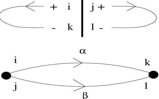
FIG. 11.: Contribution to $E_{1}^{(2)}$ in second-order perturbation theory. Top: real space representation showing sites $i$ and $j$ near the wall where the excitations are created and sites $k$ and $l$ where they are destroyed. Bottom: Feynmann diagram representation.

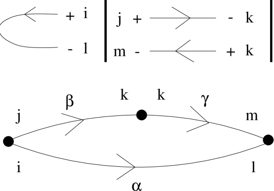
FIG. 12.: Contribution to the energy of a two-wall configuration from third-order perturbation theory. In the real space representation excitations are created at sites $i$ and $j$ and ultimately destroyed at sites $l$ and $m$ all near the left wall.

FIG. 13.: Contributions to $\delta V$ as per Eq. (89) in which the excitation to the left of the wall propagates. Nonpropagating contributions are similar to those in Fig. 7. Note that only the term in which $i$ and $l$ are nearest neighbors actually appears. Each diagram occurs four times: twice at one wall by interchanging creation and annihilation sites, and twice for interchanging the roles of the two walls.

FIG. 14.: Leading contribution to $V_{2}(n)$ for a three-dimensional system. Here $r_{\perp}$ and $s_{\perp}$ denote vectors in the plane of the wall.

FIG. 15.: Example of a term contributing to $V_{3}(2,2)$ in third order perturbation theory.

FIG. 16.: Processes which can not occur when the wall is as shown and which therefore carry a factor $\delta_{\eta,-1}$ (when the wall is absent $\eta=-1$ and these processes are allowed). The first six diagrams contribute to $V_{3}(2,2)$ and the last one to $V_{3}(2,3)$. In the last diagram the right-hand block contains three down spins.

FIG. 17.: Terms which contribute to (a) $V_{4}^{(1)}(2,2)$, (b) $V_{4}^{(2)}(2,2)$, (c) $V_{4}^{(3)}(2,2)$. The figures indicate which spins are excited. The way in which all possible orderings of the excitations are accounted for is described in the text (see equations (A8) and (A9) for diagrams (a) and (c) and equation (A10) for diagram (b)). In cases (a) and (b) the diagrams which are mirror images in the center wall must also be accounted for by including a factor of 2.

REFERENCES

- [1] Rare Earth Magnetism Structures and Excitations. J. Jensen and A. R. Mackintosh (Oxford University Press, Oxford 1991).
- [2] A. Loiseau, G Van Tendeloo, R Portier and F Ducastelle, J. Phys. (Paris) 46, 595 (1985).
- [3] P. Krishna (ed.), J. Cryst. Growth Charact. 7 (1984).
- [4] M. E. Fisher and A. M. Szpilka, Phys. Rev. B 36, 5343 (1987); A. M. Szpilka and M. E. Fisher, Phys. Rev. Lett. 57, 1044 (1986).
- [5] R. J. Elliott, Phys. Rev. 124, 346 (1961); J. M. Yeomans, in Solid State Physics, 41 (H. Ehrenreich and D. Turnbull eds, Academic Press, Orlando, 1988); W. Selke, Phys. Report 170, 213 (1988); W. Selke in Phase transitions and Critical Phenomena vol. 15, eds C. Domb and J. L. Lebowitz, (New York: Academic, 1992).
- [6] P. Bak and J. von Boehm, Phys. Rev. B.21, 5297 (1980).
- [7] M. E. Fisher and W. Selke, Phys. Rev. Lett. 44, 1502 (1980); M. E. Fisher and W. Selke, Philos. Trans. R. Soc. (London), A 302, 1 (1981).
- [8] J. Villain and M. B. Gordon, J. Phys. C. 13, 3117 (1980).
- [9] E. F. Shender, Soviet Physics, JETP 56, 178 (1982).
- [10] C. Henley, Phys. Rev. Lett. 62, 2056 (1989).
- [11] M. J. de Oliveira and R. B. Griffiths, Surf. Sci. 71, 687 (1978).
- [12] C. Micheletti, unpublished.
- [13] F. J. Dyson, Phys. Rev. 102, 1217, 1230 (1956).
- [14] S. V. Maleev, Sov. Phys. – JETP 6, 776 (1958).
- [15] As Dyson has shown [[13]] the effect of spin-wave interactions () is essentially proportional to the density of spin excitations. In fact, has NO effect on states containing a single spin excitation. On these grounds we expect that spin-wave interactions can be neglected in the present context.
- [16] P. M. Duxbury and J. M. Yeomans, J. Phys A 18, L983 (1985).
- [17] Quantum Mechanics A. Messiah. (North-Holland, Amsterdam 1966 ).
- [18] A. B. Harris, C. Micheletti and J. M. Yeomans, Quantum Fluctuations in the ANNNI Model, to be published in Physical Review Letters.
- [19] K. E. Bassler, K. Sasaki, and R. B. Griffiths, J. Stat. Phys. 62, 45 (1991).
- [20] F. Seno and J. M. Yeomans, Phys. Rev. B 50, 10385 (1994)
- [21] C. Micheletti and J. M. Yeomans, Europhys. Lett. 28, 465 (1994).
- [22] R. J. Elliott, J. A. Krumhansl, and P. L. Leath, Rev. Mod. Phys. 46, 465 (1974).