IPNO/TH 94-30
Single-particle density of states, bound states, phase-shift flip,
and a resonance in the presence of an Aharonov-Bohm potential

abstract

Both the nonrelativistic scattering and the spectrum in the presence of the Aharonov-Bohm potential are analyzed and the single-particle density of states for different self-adjoint extensions is calculated. The single-particle density of states is shown to be a symmetric and periodic function of the flux which depends only on the distance from the nearest integer. The Krein-Friedel formula for this long-ranged potential is shown to be valid when regularized with the $\zeta$ function. The limit when the radius $R$ of the flux tube shrinks to zero is discussed. For $R\neq 0$ and in the case of an anomalous magnetic moment $g_{m}>2$ (note, e. g., that $g_{m}=2.002\ 32$ for the electron) the coupling for spin-down electrons is enhanced and bound states occur in the spectrum. Their number does depend on a regularization and generically does not match with the number of zero modes in a given field that occur when $g_{m}=2$. Provided the coupling with the interior of the flux tube is not renormalized to a critical one neither bound states nor zero modes survive the limit $R\rightarrow 0$. The Aharonov-Casher theorem on the number of zero modes is corrected for the singular field configuration. Whenever a bound state does survive the $R\rightarrow 0$ limit it is always accompanied by a resonance. The presence of a bound state manifests itself in the asymmetric differential scattering cross section that can give rise to the Hall effect. The Hall resistivity is calculated in the dilute vortex limit. The magnetic moment coupling and not the spin is shown to be the primary source for the phase-shift flip that may occur even in its absence. The total energy of the system consisting of particles and field is discussed. An application to persistent currents in the plane for both spinless and spin one-half fermions is given. Persistent currents are also predicted to exist in the field of a cosmic string. The $2nd$ virial coefficient of anyons with a short range $\delta$-function interaction is calculated. The coefficient is shown to be remarkably stable when such an interaction is switched on. Several suggestions for new experiments are given.

PACS numbers : 03.65.Bz, 03-80.+r, 05.30.-d, 73.50.-h

1 Introduction

In this paper we shall report on several physical phenomena and calculate several quantities in the presence of the Aharonov-Bohm (AB) potential [1], which, in the radial gauge, is given by

$$A_{r}=0,\hskip 28.45274ptA_{\varphi}=\frac{\Phi}{2\pi r}=\frac{\alpha}{2\pi r}\,\Phi_{0}.$$ (1)

Usually, $\Phi=\alpha\,\Phi_{0}$ is the total flux through the flux tube and $\Phi_{0}$ is the flux quantum, $\Phi_{0}=hc/|e|$. The AB potential will be considered here in a more general sense since formally the same potential (of nonmagnetic origin) is generated around a cosmic string. The parameter $\Phi$ is then $1/Q_{Higgs}$, $\alpha=e/Q_{Higgs}$, and $\Phi_{0}=2\pi/e$ in the units $\hbar=c=1$ with $e$ and $Q_{Higgs}$ being respectively the charge of a test particle and the charge of the Higgs particle [2]. Experimentally, the situation of an infinitely thin flux tube is realized when a flux tube has a radius $R$ which is negligibly small when compared to all other length scales in the system. Therefore, both a flux tube with a nonzero and the zero radius will be considered. In the case when $R>0$, we shall allow generally for some additional interaction inside a flux tube, since such an interaction arises, for example, in the case of the magnetic moment coupling. The limit $R\rightarrow 0$ will then depend on the physics inside the flux tube. In a rigorous mathematical sense, different physics inside the flux tube will be described by different Hamiltonians given as a certain self-adjoint extension of a formal differential operator.

First we shall concentrate on the calculation of the single-particle density of states (DOS). The reason is that the DOS is the quantity of basic interest and provides an important link between different physical quantities. Knowledge of the DOS determines [via the Laplace transform, see Eq. (138) below] the partition function $Z(\beta)$, virial coefficients, and in the case of the Dirac equation a relation between effective energy, induced fermion number, and the axial anomaly [3, 4]. It has been used [5] to calculate the persistent current of free electrons induced in the plane by the AB potential [6]. The DOS will be calculated in two different ways: first, directly through the resolvent and second, by only using the scattering properties of the AB potential. After the DOS and differential scattering cross sections are calculated various applications are discussed.

The plan of the paper is as follows. We shall start with the case of the impenetrable flux tube when the flux tube is exterior to the system. In Sec. 2 the basic facts about the nonrelativistic AB scattering in this case are summarized. There are neither bound states nor zero modes and the DOS is determined solely in terms of the continuous spectrum. The single-particle DOS is calculated there directly from the resolvent. One finds that for integer $\alpha$ resolvents do differ by a phase factor. However, when the arguments coincide they are identical and they do have the same trace and yield a DOS identical to that in free space. We shall confirm the anticipation of Comtet, Georgelin, and Ouvry [7] that the change of the DOS is concentrated at the zero energy [see Eq. (22) below].

Different self-adjoint extensions in the case of a penetrable flux tube are discussed in Sec. 3. Let the coupling constant be negative, $e=-|e|$. Then different self-adjoint extensions arise because, in the channels $l\!=\!-n$ and $l\!=\!-n-1$, where $n$ is the integer part of $\alpha$, there are two linearly independent square integrable at zero solutions of an eigenvalue equation. These two channels are also the only two channels where a bound state can occur. Bound states are shown to parametrize different self-adjoint extensions and the change in the conventional phase shifts. Calculation of the change $\triangle_{l}$ is reviewed. Knowledge of the phase shift is then used in Sec. 4 to calculate the S matrix and scattering cross sections. The S matrix is shown to depend nontrivially on $\alpha$ and not to be a periodic function of $\alpha$. Nevertheless, the S matrix gives rise to differential and transport scattering cross sections which are periodic functions of $\alpha$ with period $1$. In the presence of a bound state, one finds in contrast to the case of the impenetrable flux tube that the differential scattering cross section ceases to be symmetric with respect to the substitution $\varphi\rightarrow-\varphi$ [see Eq. (62)], where $\varphi$ is a scattering angle. The asymmetry is easy to understand because (for $\alpha\geq 0$) bound states are only formed in the channels for which $l\leq 0$. The results are then used in Sec. 5 where the validity of the Krein-Friedel formula [8, 9] for the DOS is established for a singular potential. It is shown that the Krein-Friedel formula when regularized with the $\zeta$ function gives the correct DOS. This enables us to calculate the DOS for different self-adjoint extensions. The Krein-Friedel formula gives the DOS as the sum over phase shifts [see Eq. (65)] and thereby relates the DOS directly to the scattering properties. It is therefore very useful to have its extension to singular (especially Coulomb) potentials. One finds that whenever a bound state is present in the spectrum it is always accompanied by a resonance [Eq. (70)]. Rather surprisingly, the shape of the resonance [given in Eq. (71)] is not of the Breit-Wigner form. Since the latter is a direct consequence of analyticity it poses an interesting question on the analytic structure of scattering amplitudes for singular potentials. The existence of the resonance is quite unexpected. It will influence the transport properties of electrons in the currently almost accessible experimental regime [10], and the persistent current of free electrons in the plane [5]. In the limit of a zero energy bound state the resonance goes to zero, too, where it merges with the bound state into the continuous spectrum leaving behind the phase-shift flip.

In Sec. 6 the calculation of the number of bound states for a flux tube of finite radius $R\neq 0$ is given. The situation is considered where a short-range potential is placed inside the flux tube. The motivation is that vortices that can be realized in real experiments, such as in a superconductor of type II, definitely do have a nonzero radius. Another realistic realization of the penetrable flux tube is that suggested originally by Rammer and Shelankov [11] and later realized experimentally by Bending, Klitzing, and Ploog [10], i. e., to put a type II superconducting gate on top of the heterostructure containing the two-dimensional electron gas (2DEG) (see Fig. 1).

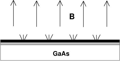
Figure 1: Black layer is a superconductor of type II put on top of the heterostructure containing the two-dimensional electron gas (shaded region). When this sample is put in a homogeneous magnetic field, magnetic field penetrates the superconductor in Abrikosov vortices. Therefore, electrons from the heterostructure do not move in the homogeneous magnetic field but in the field of a penetrable flux tube.

When a magnetic field is switched on the conventional superconductor is penetrated by vortices of flux with $\alpha=1/2$. Therefore, electrons from the heterostructure do not move in the homogeneous magnetic field but in the field of a penetrable flux tube. Electrons can penetrate to their core, in which case the potential arises as the result of the magnetic moment coupling. If the gyromagnetic ratio $g_{m}$ is less than $2$, $g_{m}<2$, the coupling with magnetic field is not sufficiently strong enough to form bound states. If the gyromagnetic ratio $g_{m}$ is exactly equal to $2$ (i. e., the magnetic moment is not anomalous) zero modes may occur in the spectrum [12, 13]. Their number equals, respectively, $n-1$ or $n$, where $n$ is the integer part of $\alpha$, depending on whether the flux is an integer or not. There is no zero mode for $\alpha\leq 1$ [12, 13]. In the region $g_{m}>2$, i.e., exactly where the gyromagnetic ratio of electron ($g_{m}=2.002\ 32$) lies, the coupling with magnetic field is enhanced and bound states do occur. In contrast to zero modes [12] one finds that the number of bound states does depend on a regularization. For example, in the case of the cylindrical shell regularization [14] their number is generally higher than for the homogeneous field regularization [see Eq. (102)]. The differences are attributed to the different energies of magnetic field inside the flux tube. In any case, however, the number of bound states does not match with the number of zero modes. The question about the existence of a bound state in the $l\!=\!-n-1$ channel is discussed. Although generally it is true that only one bound state is present for $0<\alpha<1$, provided $1-\alpha$ is sufficiently small, the second bound state does appear (cf. Ref. [15]).

An interpretation of different self-adjoint extensions and the $R\rightarrow 0$ limit are studied in Sec. 7. The existence of a critical coupling is established. In the case of the magnetic moment interaction with the interior of the flux tube, the critical coupling corresponds to the case of the normal magnetic moment with the gyromagnetic ratio $g_{m}=2$. Provided the coupling with the interior of the flux tube is weaker, bound states do not form at all. If the coupling is stronger than the critical value, then, although bound states do exist for any $R\neq 0$, they disappear in the limit $R\rightarrow 0$. Although it might seem surprising at first, the fact is a translation of the result of Berezin and Faddeev [16] established more than $30$ years ago that the nontrivial $R\rightarrow 0$ limit of a potential formally given by the Dirac delta function $\delta({\bf r})$ requires a renormalization of the coupling with the interior of the flux tube (see Ref. [17] for more details). Reference [18] provides some other examples when one encounters the necessity of a renormalization in the quantum mechanics. At first sight the renormalization might seem to be artificial and only a mathematical obscurity. However, one knows that the anomalous magnetic moment always has a form factor that does depend on the energy [19]. Therefore, in the realistic situation the renormalization is provided by nature itself.

The point spectrum [20] at the critical coupling is also considered. One finds that in the limit $R\rightarrow 0$ there are no zero modes in the AB potential for any $\alpha$. The Aharonov-Casher and the index theorems [12, 13, 21] are corrected in the sense that they do not give, respectively, the actual number of zero modes in a given finite-flux background but rather an upper bound. In the presence of a singular field configuration such as the AB potential, the square integrability of solutions must also be checked at the position of a singularity of the field. It is shown that at such a point the square integrability fails. Another argument showing why it happens is to note that the only two channels in the $R\rightarrow 0$ limit where the spectrum can differ from the conventional one are $l\!=\!-n$ and $l\!=\!-n-1$. However, for $R\neq 0$ zero modes [see Eq. (88)] only occur in channels $0\geq l\geq-n+1$, and hence they are never present in those described above.

In the presence of a bound state the conventional phase shift (7) acquires a generally energy dependent contribution (36). In the limit $R\rightarrow 0$ bound states are possible in two different channels, $l\!=\!-n$ and $l\!=\!-n-1$. However, when $R\neq 0$, the bound state does not occur generally in the $l\!=\!-n-1$ channel. Therefore, it is natural to expect that the phase-shift flip occurs generally only in the $l\!=\!-n$ channel. According to this discussion the conditions for the occurrence of the phase-shift flip given by Hagen [14] are necessary but not sufficient. Moreover, since the origin of the attractive potential inside the flux tube can be arbitrary, our calculation shows [Eqs. (34) and (68)] that the phase-shift flip occurs even in the absence of the spin. Also, in the case of particles with a spin it is not the spin but the magnetic moment coupling that is the primary source for the phase-shift flip. A nice interpretation of the phase-shift flip appears if the bound state energy is renormalized to zero. The phase-shift flip then occurs as the result of merging the bound state and the resonance into the continuous spectrum. Although the observation of the phase shift flip is usually attributed to Hagen [14], it was observed earlier in a complementary situation: in the scattering off a general two-dimensional magnetic field satisfying the finite-flux condition in the long-wavelength limit (see Ref.  [22], pp. 437 and 438). A duality can be observed [see Eq. (109)], important from the experimental point of view. Imagine two flux tubes with different radii which are otherwise negligibly small when compared to other length scales in the system. Then the scattering properties of the flux tube with a radius $R_{1}$ at momentum $k_{1}$ are the same as that of radius $R_{2}$ at momentum $k_{2}$, provided that $k_{1}R_{1}=k_{2}R_{2}$.

Starting from the next section applications to the total energy of the system (particles and a magnetic field), the Hall effect, a persistent current, and the $2$nd virial coefficients are considered. We shall show that our results are not only of academic but also of practical interest thanks to the recent developments in the fabrication of microstructures and in mesoscopic physics (see Ref. [23] for a recent review). The total energy of the system and its stability against magnetic field creation are discussed in Sec. 8. In general the diamagnetic inequality [24] tells us that that the matter is stable. The latter was proven under the assumption of minimal coupling. In our calculations we shall allow for a speculation that the magnetic moment is independent of momenta. We shall ignore the fact that the anomalous magnetic moment has a form factor that vanishes at high momenta. Under these hypotheses one can show that in the nonrelativistic case in $2+1$ dimensions, a window may exist for the magnetic moment $g_{m}>2$ in which the inequality is violated. The reason is the formation of bound states that decouple from the Hilbert space by taking away negative energy. Although the dynamics, return fluxes, and the form factor must all play an important role in the full (quantum-field theory) discussion of the stability, our relation (112) is nevertheless interesting because it gives the stability condition in terms of the ratio of the rest and the electromagnetic energies.

In Sec. 9 we shall examine consequences of the asymmetry of differential scattering cross sections. The asymmetry has important consequences as it give rise to the Hall effect. The Hall resistivity is then calculated in the dilute vortex limit [see Eq. (116)], i. e., when the multiple-scattering contribution is ignored. In Sec. 10 the results are applied to the persistent current of free electrons in the plane pierced by a flux tube. Both the spinless and the spin one-half cases are dicussed. The above mentioned resemblence between the electromagnetic AB potential and the field produced by a cosmic string [2] will enable us to conclude that the persistent current might appear in the latter case, too. Once again condensed matter physics gives both the motivation and provides a test laboratory for a phenomenon that can occur at different length scales in the Universe. Finally, in Sec. 11, the $2nd$ virial coefficient of anyons interacting with a pairwise interaction proportional to the Dirac $\delta$ function is calculated. Note that such an interaction appears in the nonrelativistic limit of planar field theories [25, 26]. It will be shown that the $2$nd virial coefficients are remarkably stable when the interaction is switched-on. The calculation is performed directly in the continuum without any use of the customary devices that makes the energy levels discrete, such as a finite box [27] or harmonic potential regularization [7, 28]. We shall show that the use of the $\zeta$-function regularization reproduces the correct answer for the $2$nd virial coefficients of noninteracting anyons [7, 27], and generalizes results of Blum et al. [28] for nonrelativistic spin one-half anyons.

Note that one has the unitary equivalence between a spin $1/2$ charged particle in a two-dimensional (2D) magnetic field and a spin $1/2$ neutral particle with an anomalous magnetic moment in a 2D electric field [29]. In our presentation we confine ourselves essentially to the nonrelativistic Schrödinger and Pauli equations. The results for the Dirac and the Klein-Gordon equations, the induced fermion number, the relation between the phase-shift flip and the axial anomaly, and the DOS in the spacetime of a gravitational vortex in $2+1$ dimensions [30] are discussed elsewhere [4]. For the problems related to the gauge transformations that are not discussed here we refer to the review of Ruijsenaars [31].

2 Impenetrable flux tube and the density of states

Let us start with the nonrelativistic case and an impenetrable flux tube. We shall consider the Pauli Hamiltonian,

$$H=\frac{({\bf p}-\frac{e}{\hbar c}{\bf A})^{2}}{2m}-\hat{\mbox{\boldmath$\mu$}}\cdot{\bf B},$$ (2)

where $\hat{\mbox{\boldmath$\mu$}}=\mu\hat{{\bf s}}/s$ is the magnetic moment operator, $\hat{{\bf s}}$ is the spin operator, and $s$ is the magnitude of the particle spin. For an electron $\mu_{e}=-g_{m}|e|\hbar/4mc=-\mu_{B}g_{m}/2$, where $\mu_{B}$ is the Bohr magneton and $g_{m}$ is the gyromagnetic ratio that characterizes the strength of the magnetic moment [19]. Naively $g_{m}=2$ but one knows that within quantum electrodynamics $\mu_{e}$ acquires radiative corrections which depend on the fine structure constant $\alpha_{\mbox{\tiny QED}}$ ($=1/137$). Within this framework we have [see Eq. (118.4) of Ref. [19]]

$$\mu_{e}=\frac{e\hbar}{2mc}\left(1+\frac{\alpha_{\mbox{\tiny QED}}}{2\pi}-0.328\frac{\alpha_{\mbox{\tiny QED}}^{2}}{\pi^{2}}\right).$$ (3)

By separating the variables and assuming $e=-|e|$, the total Hamiltonian is written as a direct sum, $H=\oplus_{l}H_{l}$, of channel radial Hamiltonians $H_{l}$ in the Hilbert space $L^{2}[(0,\infty),rdr]$ [1, 31],

$$H_{l}=-\frac{d^{2}}{dr^{2}}-\frac{1}{r}\frac{d}{dr}+\frac{\nu^{2}}{r^{2}}+g_{m}\frac{\alpha}{r}\,s_{z}\delta(r).$$ (4)

Here $\nu=|l+\alpha|$, $\alpha$ is the total flux $\Phi$ in the units of the flux quantum $\Phi_{0}=hc/|e|$, and $s_{z}=\pm 1/2$ is the projection of the spin on the direction of the flux tube [1, 31]. The Schrödinger equation is recovered upon setting $s_{z}=0$.

In the case of the impenetrable flux tube the spectra of both the Pauli and the Schrödinger equations are identical. Let us first consider the conventional setup where wave functions are zero at the position of the flux tube. There are neither zero modes nor bound states in this case as they are incompatible with the boundary conditions. To discuss the spectrum, note that for positive (negative) energies the eigenvalue equation in the $l$th channel reduces to the (modified) Bessel equation of the order $\nu=|l+\alpha|$,

$$H_{l}\psi_{l}=k^{2}\psi_{l},$$ (5)

with $k=\sqrt{2mE}/\hbar$. The boundary condition selects only regular solutions at the origin and the “spectrum” is given by

$$\psi_{l}(r,\varphi)=J_{|l+\alpha|}(kr)e^{il\varphi}.$$ (6)

Generically, to specify the boundary conditions at infinity (or at zero) is necessary only for those $l$ for which all solutions of (5) are square integrable at infinity (or at zero): the so-called limit circle case (see Ref. [32], p. 152). In general, square integrability takes the place of boundary conditions at infinity (or at zero) if one of the solutions of (5) is not square integrable at infinity (or at zero): the so-called limit point case (see Ref. [32], p. 152). From the rigorous point of view, one can speak about an impenetrable flux tube only provided that $\alpha$ is not an integer. Then all wave functions $\psi_{l}$ (6) are zero at the origin. Since $J_{0}(0)=1$, this is not the case for a flux tube with an integer flux and the physics may be different from that in free space. In what follows, we shall ignore this subtlety, and assume that the $l=0$ channel wave function $\psi_{l}$ (6) is in the spectrum, and even in this case we shall call the flux tube an impenetrable flux tube.

The AB potential (1) is long-ranged and the conventional phase shifts $\delta_{l}$’s [1],

$$\delta_{l}=\frac{1}{2}\,\pi(|l|-|l+\alpha|),$$ (7)

are singular: they do not depend on the energy and do not decay to zero for $E\rightarrow\infty$. Relation (7) can be intuitively understood as follows. The AB potential creates “vorticity” $-\alpha$, and positive and negative angular momentum wave functions “go around” the origin, respectively, in the anticlockwise and the clockwise directions [31].

The DOS will be calculated directly from the resolvent (the Green function) $G_{\alpha}({\bf x},{\bf y},E+i\epsilon)$ according to the formula

$$\rho_{\alpha}(E)=-\frac{1}{\pi}\,\mbox{ImTr}\,G_{\alpha}({\bf x},{\bf x},E+i\epsilon).$$ (8)

The integrated density of states $N_{\alpha}(E)$ is then as usual given by

$$N_{\alpha}(E)=\int_{-\infty}^{E}\rho_{\alpha}(E^{\prime})\,dE^{\prime}.$$ (9)

The eigenfunction expansion for the resolvent in polar coordinates ${\bf x}=(r_{x},\varphi_{x})$ is [33]

$$G_{\alpha}({\bf x},{\bf y},E)=\frac{m}{\pi\hbar^{2}}\int_{0}^{\infty}\frac{kdk}{q^{2}-k^{2}}\sum_{l=-\infty}^{\infty}e^{il(\varphi_{x}-\varphi_{y})}J_{|l+\alpha|}(kr_{x})J_{|l+\alpha|}(kr_{y}).$$ (10)

By using Eq. (8), one can check that the resolvent (10) gives the two-dimensional free density of states $\rho_{0}(E)=(m/2\pi\hbar^{2})V$ for $\alpha=n\in Z$, i. e., when $\alpha$ is an integer, with $V=\int d^{2}\,{\bf r}$ being the infinite volume. In the latter case, the sum in Eq. (10) can be taken exactly by means of Graf’s addition theorem (Ref. [34], relation 9.1.79),

$$\sum_{l=-\infty}^{\infty}e^{il(\varphi_{x}-\varphi_{y})}J_{|l+\alpha|}(kr_{x})J_{|l+\alpha|}(kr_{y})=e^{-in(\varphi_{x}-\varphi_{y})}J_{0}(k|{\bf x}-{\bf y}|).$$ (11)

By taking the integral in Eq. (10) (assuming that $q^{2}=q^{2}+i\epsilon$, and $r_{x}<r_{y}$) one finds

$$\int_{0}^{\infty}\frac{kdk}{q^{2}-k^{2}}J_{0}(k|{\bf x}-{\bf y}|)=-i\frac{\pi}{2}H^{(1)}_{0}(q|{\bf x}-{\bf y}|).$$ (12)

Therefore,

$$G_{n}({\bf x},{\bf y},E)=-i\frac{m}{2\hbar^{2}}\,e^{-in(\varphi_{x}-\varphi_{y})}H^{(1)}_{0}(q|{\bf x}-{\bf y}|).$$ (13)

One can also perform the integral

$$\int_{0}^{\infty}\frac{kdk}{q^{2}+i\epsilon-k^{2}}J_{\nu}(kr_{x})J_{\nu}(kr_{y})=-\frac{\pi i}{2}J_{\nu}(qr_{x})H^{(1)}_{\nu}(qr_{y})$$ (14)

first and then take the remaining sum with the same result (13). Note that Eq. (14) is also valid for nonintegral $\nu$. The Bessel functions are analytic functions and the integrals in Eqs. (12) and (14) are taken simply by the residue theorem by using a suitable contour in the complex plane (see Fig. 2 and Appendix A).

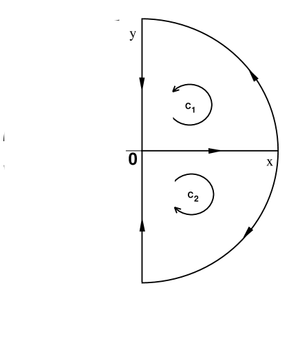
Figure 2: Contours of integration in the complex plane.

From the ‘formal scattering’ point of view taking the residue at $k=|q|+i\epsilon$ corresponds to choosing outgoing boundary conditions. From the point of view of $L^{2}[(0,\infty),rdr]$ it corresponds to taking the boundary value of the resolvent operator on the upper side of the cut at $[0,\infty)$ in the complex energy plane [35]. Note that

$${\cal G}^{+}_{l}({\bf x},{\bf y},E)=-i\frac{m}{2\hbar^{2}}\,e^{il(\varphi_{x}-\varphi_{y})}J_{\nu}(qr_{x})H^{(1)}_{\nu}(qr_{y})$$ (15)

is the resolvent of $H_{l}$ in the upper-half of the complex plane of $q$ [35]. $J_{\nu}(qr_{x})$ is square integrable (in the measure $rdr$) near the origin, and $H^{(1)}_{\nu}(qr_{y})$ is square integrable near infinity. Obviously, the resolvent is not defined for real positive $q$ since there is no solution of the Bessel equation that is square integrable at infinity for such $q$ [35] (see also asymptotic formulas in Appendix B). The point spectrum in a strict sense is empty. The spectrum is purely continuous and lies on $[0,\infty)$ where the partial resolvent ${\cal G}^{+}_{l}$ (the Fourier transform of the retarded Green function) has a cut [35]. The partial resolvent ${\cal G}^{-}_{l}$ in the lower-half of the complex plane (the Fourier transform of the advanced Green function) is the complex conjugate of ${\cal G}^{+}_{l}$ [35],

$${\cal G}^{-}_{l}({\bf x},{\bf y},E)=i\frac{m}{2\hbar^{2}}\,e^{-il(\varphi_{x}-\varphi_{y})}J_{\nu}(qr_{x})H^{(2)}_{\nu}(qr_{y}).$$ (16)

Note that the total Green function $G_{n}({\bf x},{\bf y},E)$ in the presence of an integer flux $n\neq 0$ [see Eq. (13)] differs from $G_{0}({\bf x},{\bf y},E)$ by a phase factor. However, to calculate the DOS one needs the value of $G_{n}({\bf x},{\bf y},E)$ at $\varphi_{x}=\varphi_{y}$ and hence the result for the integer flux will be the same as at $\alpha=n=0$. The limiting value of the resolvent operator on the lower side of the cut is the complex conjugate of (13), the discontinuity across the cut

$$G_{n}({\bf x},{\bf x},E_{+})-G_{n}({\bf x},{\bf x},E_{-})=-i(m/\hbar^{2}),$$ (17)

and

$$-(1/\pi)\,\mbox{Im}\,G_{n}({\bf x},{\bf x},E_{+})=m/(2\pi\hbar^{2})$$ (18)

which confirms our normalization.

Whenever $\alpha\not\in Z$ Graf’s theorem cannot be used. To proceed further with this case we use the fact that (14) has an analytic continuation on the imaginary axis in the complex momentum plane

$$\int_{0}^{\infty}\frac{kdk}{q^{2}+k^{2}}J_{\nu}(kr_{x})J_{\nu}(kr_{y})=\frac{\pi i}{2}J_{\nu}(iqr_{x})H^{(1)}_{\nu}(iqr_{y})=I_{\nu}(qr_{x})K_{\nu}(qr_{y}),$$ (19)

where $I_{\nu}$ and $K_{\nu}$ are modified Bessel functions [34]. One can obtain this result either by performing the integral directly or by performing the analytic continuation in (14). To sum over $l$ one uses the integral representation of these functions [34, 36]. Following the steps given in Ref. [37] one can separate the $\alpha$-dependent contribution

$$\triangle G_{\alpha}({\bf x},{\bf x},E)=G_{\alpha}({\bf x},{\bf x},M)-G_{0}({\bf x},{\bf x},M)=$$ (20)

$$-\frac{m}{\hbar^{2}}\frac{\sin(\eta\pi)}{(2\pi)^{2}}\int_{-\infty}^{\infty}\!d\vartheta\,\int_{-\infty}^{\infty}\!d\omega e^{-Mr_{x}(\cosh\vartheta+\cosh\omega)}\,\frac{e^{\eta(\vartheta-\omega)}}{1+e^{\vartheta-\omega}},$$

where $M=-i\sqrt{2mE}/\hbar$ and $\eta$ is the nonintegral part of $\alpha$, $0\leq\eta<1$. After taking the trace over spatial coordinates, using formulas 3.512.1 and 8.334.3 of Ref. [36] (see Appendix A), and returning back to the real momentum axis, one finally finds

$$\mbox{Tr}\,\triangle G_{\alpha}({\bf x},{\bf x},E)=-\eta(1-\eta)\frac{1}{2E}\cdot$$ (21)

Hence, the change $\triangle\rho_{\alpha}(E)=\rho_{\alpha}(E)-\rho_{0}(E)$ of the DOS induced by the AB potential in the whole space is concentrated at zero energy where it is proportional to the $\delta$ function,

$$\triangle\rho_{\alpha}(E)=-\frac{1}{\pi}\,\mbox{ImTr}\,\triangle G_{\alpha}({\bf x},{\bf x},E_{+})=-\frac{1}{2}\,\eta(1-\eta)\,\delta(E).$$ (22)

This result is similar to the result (135) that was obtained in the context of anyonic physics [7] (see also Sec. 11 below). The same term has been obtained by Berry [38] as the leading term in the semiclassical approximation to the change of the DOS for the AB (circular, heart shaped, and Africa shaped) quantum billiards. Thereby, the semiclassical approximation turns out to be exact in the $R\rightarrow\infty$ limit, where $R$ is the characteristic length of the billiards.

Let us now take the case where $\alpha$ is negative and of the form $\alpha=-n-\eta\leq 0$ where $n\geq 0$ is a positive integer and $\eta$ (the fractional part of $\alpha$) satisfies $0\leq\eta<1$. One can readily repeat the same procedure to obtain the change in the DOS. The result is exactly the same as in (22),

$$\triangle\rho_{-\alpha}(E)=\triangle\rho_{\alpha}(E)=-\frac{1}{2}\,\eta(1-\eta)\,\delta(E).$$ (23)

Therefore, $\triangle\rho_{\alpha}(E)$ as a function of $\alpha$ is a symmetric function under the transformation $\alpha\rightarrow-\alpha$. Moreover, one can show that $\triangle\rho_{\alpha}(E)$ as a function of $\alpha$ is only a function of a distance from the nearest integer. Indeed, under the substitution

$$\eta^{\prime}=1-\eta$$ (24)

one finds that $\triangle\rho_{\alpha}(E)$ is form invariant, namely

$$\triangle\rho_{\alpha}(E)=-\frac{1}{2}\,\eta(1-\eta)\,\delta(E)=-\frac{1}{2}\,\eta^{\prime}(1-\eta^{\prime})\,\delta(E).$$ (25)

3 Penetrable flux tube and self-adjoint extensions

Physically, self-adjoint extensions in the presence of an Aharonov-Bohm potential can be understood as follows. In channels with $|l+\alpha|>1$, one has a unique choice for the resolvent of $H_{l}$ in $L^{2}[(0,\infty),rdr]$. Apart from $J_{|l+\alpha|}(kr)$, there does not exist any other linearly independent solution of Eq. (5) which is square integrable at the origin. Similarly, apart from $H_{|l+\alpha|}^{(1,2)}(kr)$, there does not exist any other linearly independent solution of Eq. (5) which is square integrable at infinity in the upper (lower) complex half-plane of $k$. In this case, the Hamiltonian $H_{l}$ is said to be in the limit point case at both infinity and the origin [32], and the square integrability takes the place of boundary conditions. An ambiguity in defining the resolvent ${\cal G}_{l}^{\pm}$ [see Eqs. (15) and (16)] of $H_{l}$ arises only in the channels with $|l+\alpha|<1$, i. e., with $l\!=\!-n,-n-1$. There are exactly those values of $l$ for which Eq. (5) has two linearly independent (and hence all) square integrable at the origin solutions. These solutions can be taken to be $J_{|l+\alpha|}$ and $J_{-|l+\alpha|}$. Then, if $J_{|l+\alpha|}(qr_{x})$ is replaced in either (15) or (16) by any linear combination of $J_{|l+\alpha|}(qr_{x})$ and $J_{-|l+\alpha|}(qr_{x})$, one obtains a well defined resolvent of $H_{l}$. To any particular choice of the linear combination corresponds a particular self-adjoint extension of $H_{l}$. For these values of $l$, the AB potential is said to be in the limit circle case at zero (see Ref. [32], p. 152), and boundary conditions at the origin must be specified to define a resolvent uniquely.

From the formal mathematical point of view the above discussion is repeated as follows. Formal differential operator $H_{l}$ in $L^{2}[(0,\infty),rdr]$ is real and hence commutes with the involution operator (complex conjugation) in the Hilbert space. Therefore, by the von-Neumann theorem (see Ref. [32], p. 143), when $H_{l}$ is defined as a symmetric operator on a dense set in $L^{2}[(0,\infty),rdr]$ such as $C^{\infty}_{0}(0,\infty)$ (the set of infinitely differentiable functions that are zero at the origin and decay exponentially at infinity) it always can be extented to a self-adjoint operator. According to theorem X.11 of Ref. [32], except for the channels with $|l+\alpha|<1$, the operators $H_{l}$ are already essentially self-adjoint on $C^{\infty}_{0}(0,\infty)$ [their deficiency indices are $(0,0)$]. Only the operators $H_{l}$ with $|l+\alpha|<1$, i. e., with $l\!=\!-n,-n-1$, admit a nontrivial one-parametric family of self-adjoint extensions [31, 35] (their deficiency indices are $(1,1)$ [31]). Therefore, in these two cases the Hamiltonian as a self-adjoint operator in the Hilbert space is not defined uniquely. Different self-adjoint extensions give different Hamiltonians which correspond to different physics inside the flux tube and different boundary conditions at its boundary (see an example in Ref. [32], pp. 144 and 145).

To identify the particular self-adjoint extension one starts with the finite flux tube of radius $R$ and takes the limit $R\rightarrow 0$ (see Sec. 7). We shall consider the situation with bound states of energy $E_{l}=-(\hbar^{2}/2m)\kappa_{l}^{2}$ in the $l\!=\!-n$ and $l\!=\!-n-1$ channels, and with $n=[\alpha]$ denoting the nearest integer smaller than or equal to $\alpha$. This happens when a sufficiently strong attractive short-range potential is placed inside the flux tube. In the nonrelativistic case for spin-down fermions this is the case when their magnetic moment exceeds the value $2$ such as in the case of the electron which has $g_{m}=2.002\ 32$ [4, 39]. For negative energy, the eigenvalue equation with $H_{l}$ leads to the modified Bessel equation and the wave function is given by

$$B_{l}(r,\varphi)=K_{|l+\alpha|}(\kappa_{l}r)\,e^{il\varphi}.$$ (26)

$K_{|l+\alpha|}(\kappa_{l}r)$ decreases exponentially for $r\rightarrow\infty$ and for $|l+\alpha|<1$ it is in $L^{2}[(0,\infty),rdr]$, although it is singular at the origin (see Appendix B). Nevertheless, if we want the bound state to be in the Hilbert space the scattering states (6) in the channels $l\!=\!-n$ and $l\!=\!-n-1$ have to be modified. They become a combination of the regular and singular Bessel functions,

$$\psi_{l}(r,\varphi)=\left[J_{|l+\alpha|}(kr)-A_{l}J_{-|l+\alpha|}(kr)\right]\,e^{il\varphi}.$$ (27)

This is because $H_{l}$ has necessarily to be a symmetric operator. This means that the radial parts $\chi(r)$ of any two states $\psi_{1}({\bf r})$ and $\psi_{2}({\bf r})$ in the Hilbert space have to satisfy

$$r\,\left[\partial_{r}\chi^{*}_{1}(r)\chi_{2}(r)-\chi^{*}_{1}(r)\partial_{r}\chi_{2}(r)\right]=r\,W[\chi_{1}^{*},\chi_{2}]\rightarrow 0$$ (28)

in the limit $r\rightarrow 0$, where $W[,]$ denotes the Wronskian. The condition (28) is nothing but the boundary condition at the origin: in the limit $r\rightarrow 0$ the logarithmic derivative $r\,\chi^{\prime}(r)/\chi(r)$ of any state in the given Hilbert space takes a fixed value [40]. This is a translation of the mathematical analysis in terms of deficiency indices [31] into more physical terms. Obviously, the Wronskian will vanish when the asymptotic forms for $r\rightarrow 0$, up to order ${\cal O}(r)$, of any two states are identical. For the general scattering solution (27) for $0<\nu<1$ one has (see Appendix B)

$$J_{\nu}(kr)-AJ_{-\nu}(kr)\sim-\frac{A}{\Gamma(1-\nu)}\left[\left(\frac{kr}{2}\right)^{-\nu}-\frac{1}{A}\frac{\Gamma(1-\nu)}{\Gamma(1+\nu)}\left(\frac{kr}{2}\right)^{\nu}\right]+{\cal O}(r^{2-\nu}).$$ (29)

The asymptotic form of (26) is then determined by that of $K_{\nu}(z)$ [see Eq. (174) of Appendix B]

$$K_{\nu}(z)\sim\frac{1}{2}\Gamma(\nu)\left[\left(\frac{z}{2}\right)^{-\nu}-\frac{\Gamma(1-\nu)}{\Gamma(1+\nu)}\left(\frac{z}{2}\right)^{\nu}\right]+{\cal O}(z^{2-\nu}).$$

Therefore, the condition (28) determines $A_{l}$ in the channels $l\!=\!-n$ and $l\!=\!-n-1$ to be

$$A_{-n} = \left(k/\kappa_{-n}\right)^{2\eta}=\left(E/|E_{-n}|\right)^{\eta},$$

$$A_{-n-1} = \left(k/\kappa_{-n-1}\right)^{2(1-\eta)}=\left(E/|E_{-n-1}|\right)^{1-\eta},$$ (30)

i. e., energy dependent. According to (27) and (30) the bound state energy determines the spectrum of $H_{l}$ in the Hilbert space that is different for different bound state energies. Therefore, in physical terms, it is the bound state energy that parametrizes different self-adjoint extensions.

Quite surprisingly, the influence of the bound state on the wave function (27) is most pronounced in the limit $E_{b}\rightarrow 0$. Then $A_{l}\rightarrow\infty$ and the regular wave function changes to the singular one,

$$\psi_{l}(r,\varphi)=J_{|l+\alpha|}(kr)\,e^{il\varphi}\rightarrow\psi_{l}(r,\varphi)=J_{-|l+\alpha|}(kr)\,e^{il\varphi}.$$ (31)

On the other hand, in the limit of a bound state with infinite bound energy, $A_{l}\rightarrow 0$ and

$$\psi_{l}(r,\varphi)=\left[J_{|l+\alpha|}(kr)-A_{l}J_{-|l+\alpha|}(kr)\right]e^{il\varphi}\rightarrow$$ (32)

$$\psi_{l}(r,\varphi)=J_{|l+\alpha|}(kr)\,e^{il\varphi}.$$

By using the formula (9.2.5) of Ref. [34] one finds that the radial part of the general solution (27) behaves for $r\rightarrow\infty$ as follows:

$$R_{l}(r)\sim\mbox{const}\times\left(e^{-ikr}+\frac{1-A_{l}e^{i\pi|l+\alpha|}}{1-A_{l}e^{-i\pi|l+\alpha|}}e^{-i\pi(|l+\alpha|+1/2)}e^{ikr}\right).$$ (33)

By comparing with its behavior for $\alpha=0$ one finds the $l$th channel S_l matrix to be S${}_{l}=e^{2i\delta_{l}}$ with

$$\delta_{l}=\delta_{l}(E)=\frac{1}{2}\pi(|l|-|l+\alpha|)+\triangle_{l}(E).$$ (34)

The change $\triangle_{l}=\triangle_{l}(E)$ of the conventional phase shift (7) is determined by the equation

$$e^{2i\triangle_{l}}=\frac{1-A_{l}e^{i\pi|l+\alpha|}}{1-A_{l}e^{-i\pi|l+\alpha|}},$$ (35)

with the solution given by

$$\triangle_{l}=\arctan\left(\frac{\sin(|l+\alpha|\pi)}{\cos(|l+\alpha|\pi)-A_{l}^{-1}}\right).$$ (36)

Here we have tacitly assumed that $A_{l}\rightarrow 0$ as $\eta\rightarrow 0$. For the discussion of this point see the end of Sec. 6. Note that when the bound state energy is changed, $E_{b}\rightarrow E_{b}^{\prime}$, and consequently $\kappa\rightarrow\kappa^{\prime}$, then the phase shift $\delta_{l}(k)$ in the corresponding channel at momentum $k$ equals to $\delta_{l}^{\prime}(k^{\prime})$, the phase shift in the same channel when the bound state energy is $E_{b}^{\prime}$, provided that

$$k^{\prime}=\frac{\kappa^{\prime}}{\kappa}k.$$ (37)

The energy of the bound state breaks the classical scale invariance and sets a scale to the problem. Equation (37) then expresses the scaling transformation under which the problem is invariant.

One sees again that the most pronounced influence on the phase shift is in the limit $E_{b}\uparrow 0$. Then $A_{l}^{-1}=0$,

$$\delta_{l}=\frac{1}{2}\pi(|l|+|l+\alpha|),$$ (38)

and one has the phase-shift flip when compared to the conventional phase shift (7). Using the fact that phase shifts are only defined modulo $\pi$ one finds

$$\delta_{-n} = \frac{1}{2}\pi(n-\eta)\simeq-\frac{1}{2}\pi\alpha\rightarrow\frac{1}{2}\pi\alpha,$$

$$\delta_{-n-1} = \frac{1}{2}\pi(n+\eta)\simeq\frac{1}{2}\pi\alpha\rightarrow-\frac{1}{2}\pi\alpha.$$ (39)

4 The S matrix and scattering cross sections

Once phase shifts are calculated, the form of scattering amplitudes, the S matrix, and cross sections can be discussed. The scattering amplitude $f(k,\varphi)$ in two space dimension is defined as the coefficient in front of $e^{ikr}/r^{1/2}$ in the asymptotic expansions as $r\rightarrow 0$ of the wave function (see Ref. [41] for a more rigorous definition),

$$\psi_{l}(r,\varphi,\varphi^{\prime})\sim e^{ikr\cos(\varphi-\varphi^{\prime})}+f(k,\varphi-\varphi^{\prime})\,\frac{e^{ikr}}{r^{1/2}},$$ (40)

where $\varphi^{\prime}$ is the direction of the incident plane wave. The scattering amplitude $f(k,\varphi)$ is related to the S matrix,

$$(S-1)(k,\varphi)=(ik/2\pi)^{1/2}f(k,\varphi),$$ (41)

where $1$ stands here for the unit operator. In the partial-wave expansion one has

$$f(k,\varphi)=(2\pi ik)^{-1/2}\sum_{l=-\infty}^{\infty}\left(e^{2i\delta_{l}(k)}-1\right)e^{il\varphi},$$ (42)

which expresses the scattering amplitude in terms of the phase shifts $\delta_{l}(k)$. The differential scattering cross section is given by

$$\left(\frac{d\sigma}{d\varphi}\right)(k,\varphi)=|f(k,\varphi)|^{2}.$$ (43)

In conventional AB scattering, the phase shifts $\delta_{l}$’s are given by Eq. (7). One then finds that

$$e^{2i\delta_{l}}=\left\{\begin{array}[]{rl}e^{-i\pi\alpha},&l\geq-n\\ e^{i\pi\alpha},&l\leq-n-1,\end{array}\right.$$ (44)

where, as above, $n$ stands for the integer part, $[\alpha]$, of $\alpha$. Therefore, the S matrix, $s^{0}_{\alpha}(\varphi)$, in the AB potential is given by

$$s^{0}_{\alpha}(\varphi):=\frac{1}{2\pi}\sum_{l=-\infty}^{\infty}e^{2i\delta_{l}+il\varphi}=$$ (45)

$$\frac{\cos(\pi\alpha)}{2\pi}\sum_{l=-\infty}^{\infty}e^{il\varphi}+i\frac{\sin(\pi\alpha)}{2\pi}e^{-in\varphi}\left[\sum_{l=-\infty}^{-1}-\sum_{l=0}^{\infty}\right]e^{il\varphi},$$

where the superscript $0$ means that we are dealing with conventional AB scattering. Now, the sum in the first term in Eq. (45) gives the delta function $\delta(\varphi)$. Provided $\varphi\neq 0$ the second sum in Eq. (45) (as well as the first sum) can be taken exactly [42] and one finds that the term in parentheses gives

$$e^{-i\varphi}\frac{1}{1-e^{-i\varphi}}-\frac{1}{1-e^{i\varphi}}=2\,\frac{1}{e^{i\varphi}-1}\cdot$$ (46)

It is obviously singular at $\varphi=0$. Therefore, care has to be taken to define the sum at this point. One has to resist the temptation to extrapolate the result from those at $\varphi\neq 0$ because the result is not continuous at $\varphi=0$. One can show that the result is given by [31]

$$s^{0}_{\alpha}(\varphi)=\delta(\varphi)\cos\pi\alpha+i\,\frac{\sin\pi\alpha}{\pi}\,e^{-in\varphi}\,P\frac{1}{e^{i\varphi}-1},$$ (47)

where P denotes an analog of the principal value. Formally,

$$P\,\frac{1}{e^{i\varphi}-1}=\lim_{\epsilon\downarrow 0}\frac{1}{2}\left[\frac{1}{e^{i\varphi}-(1-\epsilon)}+\frac{1}{e^{i\varphi}-(1+\epsilon)}\right].$$ (48)

The result (47) can be verified by taking the inverse Fourier transform and using the formula

$$P\int_{-\pi}^{\pi}\!d\varphi\,\frac{e^{ik\varphi}}{e^{i\varphi}-1}=\left\{\begin{array}[]{rl}\pi,&k\geq 1\\ -\pi,&k\leq 0.\end{array}\right.$$ (49)

Note that there is nothing particular about the $\delta$ function term in the S matrix in the presence of an AB potential. In fact, $S(\varphi)=\delta(\varphi)$ is the S matrix in free space (in the absence of any scatterer), as can be checked directly by substituting $\alpha=0$ in Eq. (45). The $\delta$ function in Eq. (47) simply means that a fraction $\cos\pi\alpha$ of an incident beam passes through the flux tube without being scattered.

In the case of negative $\alpha=-|\alpha|$ the analog of (44) is

$$e^{2i\delta_{l}}=\left\{\begin{array}[]{rl}e^{i\pi|\alpha|},&l\geq n+1\\ e^{-i\pi|\alpha|},&l\leq n.\end{array}\right.$$ (50)

By repeating the above procedure leading to (47), one finds that the S matrix in the present case is

$$s^{0}_{-|\alpha|}(\varphi)=\delta(\varphi)\cos\pi|\alpha|+i\,\frac{\sin\pi|\alpha|}{\pi}\,e^{in\varphi}\,P\frac{1}{e^{-i\varphi}-1}\cdot$$ (51)

This result for $s^{0}_{-|\alpha|}(\varphi)$ can be verified independently by taking the inverse Fourier transform and using the formula

$$P\int_{-\pi}^{\pi}\!d\varphi\,\frac{e^{ik\varphi}}{e^{-i\varphi}-1}=\left\{\begin{array}[]{rl}\pi,&k\leq-1\\ -\pi,&k\geq 0.\end{array}\right.$$ (52)

A comparison of relations (47) and (51) shows that, under the transformation $\alpha\rightarrow-\alpha$,

$$s^{0}_{-|\alpha|}(\varphi)=s^{0}_{|\alpha|}(-\varphi).$$ (53)

According to Eq. (41), the scattering amplitude is given by

$$f_{\alpha}(k,\varphi)=(2\pi/ik)^{1/2}[s_{\alpha}-1](k,\varphi).$$ (54)

For $\varphi\neq 0$ one finds

$$f^{0}_{\alpha}(k,\varphi)=(1/2\pi ik)^{1/2}\frac{\sin(\pi\alpha)}{\sin(\varphi/2)}e^{-i(n+1/2)\varphi}.$$ (55)

Hence, provided $\varphi\neq 0$, one has by using Eq. (43)

$$\left(\frac{d\sigma^{0}}{d\varphi}\right)(k,\varphi)=\frac{1}{2\pi k}\frac{\sin^{2}(\pi\alpha)}{\sin^{2}(\varphi/2)}\cdot$$ (56)

The total scattering cross section is infinite for $\alpha\not\in Z$ and vanishes for $\alpha\in Z$ [31]. For the purpose of the experiment, note that the differential scattering cross section (56) is symmetric under $\varphi\rightarrow-\varphi$.

When bound states are present in the $l\!=\!-n$ and in the $l\!=\!-n-1$ channels, the S matrix and the scattering amplitude $f_{\alpha}(k,\varphi)$ are modified. First one finds that

$$s^{0}_{\alpha}\rightarrow s_{\alpha}=s^{0}_{\alpha}+\triangle s^{0}_{\alpha},$$ (57)

where

$$\triangle s^{0}_{\alpha}(\varphi)=\sum_{l=-n-1}^{-n}\left[e^{2i(\delta_{l}+\triangle_{l})}-e^{2i\delta_{l}}\right]e^{il\varphi}$$ (58)

$$=2i\sum_{l=-n-1}^{-n}e^{2i\delta_{l}+i\triangle_{l}+il\varphi}\sin\triangle_{l}.$$

Here, $\triangle_{l}$ is the change (36) of the conventional AB phase shift (7) in the channel $l$. Similarly, one introduces $\triangle f^{0}_{\alpha}(k,\varphi)$ as

$$f_{\alpha}(k,\varphi)=f^{0}_{\alpha}(k,\varphi)+\triangle f^{0}_{\alpha}(k,\varphi).$$ (59)

According to Eq. (54) one has

$$\triangle f^{0}_{\alpha}(k,\varphi)=(2i/\pi k)^{1/2}\sum_{l=-n-1}^{-n}e^{2i\delta_{l}+i\triangle_{l}+il\varphi}\sin\triangle_{l}.$$ (60)

Nevertheless, the property (53) of the S matrix still holds and even in the presence of bound states one has

$$s_{-|\alpha|}(\varphi)=s_{|\alpha|}(-\varphi).$$ (61)

To prove this it is sufficient to show that that a phase shift $\delta_{l}(E)$ in the $l\!=\!-n$ ($l\!=\!-n-1$) channel for $\alpha\geq 0$ is the same as that in the $l\!=\!n$ ($l\!=\!n+1$) channel for $\alpha\leq 0$. In the case of conventional phase shifts one can check for this property directly from Eqs. (44) and (50). Since bound state energies and $|l+\alpha|$ remain invariant under the transformation $\alpha\rightarrow-\alpha$ and $l\rightarrow-l$, according to Eq. (36), $\triangle_{l}$, and hence the phase shift (34), remains invariant, too.

Note that if $\alpha$ changes by $\pm 1$, the S matrix [see Eqs. (47) and (57)] as a function of $\alpha$ is not a periodic function of $\alpha$ and changes nontrivially. This is analogous to the fact that, as was shown in Sec. 2, the Green’s function also depends nontrivially on $\alpha$. However, such as in the latter case when the Green’s function gave the single-particle DOS which was periodic in $\alpha$ with respect to the substitution $\alpha\rightarrow\alpha\pm 1$, the S matrix will be shown to give scattering cross sections that are periodic in $\alpha$ with the same period, too. In the absence of bound states this follows immediately from Eq. (56). In the presence of bound states, the differential scattering cross section for $\varphi\neq 0$ is calculated by using Eqs. (43) and (60),

$$\left(\frac{d\sigma}{d\varphi}\right)(k,\varphi)=\left(\frac{d\sigma^{0}}{d\varphi}\right)(k,\varphi)+\frac{8\pi}{k}\sum_{l=-n-1}^{-n}\sin^{2}\triangle_{l}\,+$$ (62)

$$\frac{4}{k}\frac{\sin(\pi\alpha)}{\sin(\varphi/2)}\left[\sin\triangle_{-n}\cos\left(\triangle_{-n}-\pi\alpha+\varphi/2\right)+\sin\triangle_{-n-1}\cos\left(\triangle_{-n-1}+\pi\alpha-\varphi/2\right)\right].$$

The periodicity of the differential cross section with respect to the substitution $\alpha\rightarrow\alpha\pm 1$ then follows from Eq. (62). Note that in the presence of bound states, the differential cross section becomes asymmetric with regard to $\varphi\rightarrow-\varphi$ (what is equivalent, with regard to $\alpha\rightarrow-\alpha$). The origin of the asymmetry is easy to understand as bound states for $\alpha\geq 0$ are formed only in channels with $l\leq 0$.

For completeness we also give the result for the so-called transport scattering cross section $\sigma_{tr}$, defined by

$$\sigma_{tr}:=\int_{-\pi}^{\pi}(1-\cos\varphi)\,\frac{d\sigma}{d\varphi}\,d\varphi$$ (63)

[see Ref.  [43], Eq. (139.7)]. One finds

$$\sigma_{tr}=\frac{2}{k}\,\sin^{2}(\pi\alpha)+\frac{16\pi^{2}}{k}\sum_{l=-n-1}^{-n}\sin^{2}\triangle_{l}$$ (64)

$$-\frac{8\pi}{k}\sin(\pi\alpha)\left[\sin\triangle_{-n}\sin(\triangle_{-n}-\pi\alpha)-\sin\triangle_{-n-1}\sin(\triangle_{-n-1}+\pi\alpha)\right].$$

As is the differential scattering cross section, the transport scattering cross section is also periodic with respect to the substitution $\alpha\rightarrow\alpha\pm 1$.

5 The Krein-Friedel formula and the resonance

Now, we shall show that to calculate the change of the integrated density of states (IDOS) in the whole space, one can use the Krein-Friedel formula [8]. The latter gives the contribution $\triangle N_{\alpha}(E)$ of the scattering states to the change of the IDOS induced by the presence of a scatterer, directly as the sum over phase shifts,

$$\triangle N_{\alpha}(E)=\frac{1}{\pi}\sum_{l}\delta_{l}(E)=(2\pi i)^{-1}\ln\det\mbox{S},$$ (65)

S being the total on-shell S matrix. As has been shown in Sec. 4, the S matrix (47) is singular as a consequence of the singularity of phase shifts (34) which in general do not decay when $E\rightarrow\infty$. Therefore, the S matrix (47) or (57) cannot be substituted directly into the Krein-Friedel formula (65). This can also be seen from the fact that the sum (65) over phase shifts is not absolutely convergent. We remind the reader that the sum of a series that is not absolutely convergent is ambiguous in a conventional sense. If suitably rearranged, the (conventional) sum of such a series can take any prescribed value. Thus, to deal with such a series, care must be taken. In the present case of the AB potential we have found that it is the $\zeta$-function regularization which gives the correct answer [(22)]. In the absence of bound states

$$\ln\det\mbox{S}=\sum_{l=-\infty}^{\infty}2i\delta_{l}=i\pi\sum_{l=-\infty}^{\infty}(|l|-|l+\alpha|)$$ (66)

$$=i\pi\left[2\sum_{l=1}^{\infty}l-\sum_{l=-n}^{\infty}(l+\alpha)+\sum_{-\infty}^{-n-1}(l+\alpha)\right]$$

$$=i\pi\left.\left[2\sum_{l=1}^{\infty}l^{-s}-\sum_{l=0}^{\infty}(l+\eta)^{-s}-\sum_{l=1}^{\infty}(l-\eta)^{-s}\right]\right|_{s=-1}$$

$$=i\pi\left.\left[2\zeta_{R}(s)-\zeta_{H}(s,\eta)-\zeta_{H}(s,1-\eta)\right]\right|_{s=-1}=-i\pi\eta(1-\eta),$$

where $\zeta_{R}$ and $\zeta_{H}$ are the Riemann and the Hurwitz $\zeta$ functions (see Appendix D). Thus, by using Eq. (65), the change of the DOS is

$$\triangle\rho_{\alpha}(E)=-\eta(1-\eta)\,\delta(E)/2.$$

This result is exactly (22). Therefore, despite the AB potential being long-ranged, the Krein-Friedel formula can still be used when regularized with the $\zeta$-function. In the case where $\alpha$ is negative and equals $-n-\eta$, the calculation of the change of the DOS is essentially the same. The only change is that now

$$|l+\alpha|=\left\{\begin{array}[]{rl}l+\alpha,&l\geq n+1\\ -l-\alpha,&l\leq n.\end{array}\right.$$ (67)

By using the Krein-Friedel formula one again reproduces the result (23).

As has been discussed in Sec. 3, under the influence of bound states the phase shifts are changed only in two channels, $l\!=\!-n$ and $l\!=\!-n-1$. Therefore, the contribution of scattering states to the change of the IDOS is then

$$\triangle N_{\alpha}(E)= - \frac{1}{2}\eta(1-\eta)+\frac{1}{\pi}\arctan\left(\frac{\sin(\eta\pi)}{\cos(\eta\pi)-(|E_{-n}|/E)^{\eta}}\right)$$ (68)

$$- \frac{1}{\pi}\arctan\left(\frac{\sin(\eta\pi)}{\cos(\eta\pi)+(|E_{-n-1}|/E)^{(1-\eta)}}\right),$$

where $E_{-n}$ and $E_{-n-1}$ are the binding energies in $l\!=\!-n$ and $l\!=\!-n-1$ channels. By using the arguments given in the proof of relation (61) one finds that the presence of bound states does not spoil the property (23) of the DOS, and the IDOS is still a symmetric function of $\alpha$,

$$\triangle N_{-|\alpha|}(E)=\triangle N_{|\alpha|}(E).$$ (69)

Note that for $0<\eta<1/2$ the resonance appears at

$$E_{res}=\frac{|E_{-n}|}{\left[\cos(\eta\pi)\right]^{1/\eta}}>0.$$ (70)

The phase shift $\delta_{-n}(E)$ (34) changes by $\pi$ in the direction of increasing energy and the integrated density of states (68) has a sharp increase by $1$. The profile of the resonance [the argument of arctan in Eq. (34)] is given by

$$\frac{E^{\eta}\tan\eta\pi}{E^{\eta}-E_{res}^{\eta}}=\frac{\Gamma}{E^{\eta}-E_{res}^{\eta}},$$ (71)

where $\Gamma$ is the width of the resonance,

$$\Gamma=E_{res}^{\eta}\tan\eta\pi.$$ (72)

Note that the profile (71) is not of the Breit-Wigner form,

$$\frac{\Gamma}{E-E_{res}}$$ (73)

(see Ref.  [43], §145).

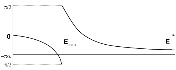
Figure 3: Typical energy dependence of $\triangle_{l}(E)$ in the channel with a bound state.

For $1/2<\eta<1$ the resonance is shifted to the $l\!=\!-n-1$ channel. $\eta=1/2$ is a special point since resonances occur in both channels at infinity. Therefore, the contribution of the arctan terms in (68) does not vanish as $E\rightarrow\infty$, but instead gives the value $-1$. Here, we have assumed that bound states are in both the $l\!=\!-n$ and $l\!=\!-n-1$ channels. As we shall see in Sec. 6, it is generally easier to form the bound state in the $l\!=\!-n$ channel than in the $l\!=\!-n-1$ channel. Therefore, unless $\eta$ is sufficiently large, only the bound state in $l\!=\!-n$ is present and the above considerations have to be appropriately modified. The above discussion also shows that even in the generic case, when bound states are present, the DOS still depends only on the distance from the nearest integer. Equation (70) shows that if the energy of the bound state goes to zero, $E_{b}\uparrow 0$, the resonance also approaches zero energy, $E_{res}\downarrow 0$. Therefore, in the limit $E_{b}\uparrow 0$ the resonance merges with the bound state. As will be discussed in more detail in Sec. 7 both the resonance and a bound state disappear from the point spectrum and leave behind the phase-shift flip.

Having calculated phase shifts (34) for a generic self-adjoint extension, one can calculate the time delay $\triangle t$ associated with the energy derivative of the phase shift [41],

$$\triangle t=2\hbar\frac{d\delta(E)}{dE}\cdot$$ (74)

One sees immediately that if $l$ is different from $-n$ and $-n-1$, then the time delay is $\triangle t=0$. The time delay (74) can be nonzero only in the channels $l=-n$ and $l=-n-1$, and at the energy corresponding to the resonance the time delay is infinite.

6 Regularization

To identify the physics that underlines different self-adjoint extensions we have considered the situation when the AB flux tube is regularized by a flux tube of a finite radius $R$, and the magnetic field $B$ inside it satisfies the constraint (87). This situation was discussed first in Ref. [44]. The discussion of this case has a direct relevance for experiment since vortices usually realized in experiments are not singular and do have a nonzero radius [10, 23, 11]. In order for a bound state to exist, the matching equation for logarithmic derivatives of the exterior (see Appendix B) and interior (see Appendix C) solutions in the $l$th channel must have a solution. The logarithmic derivative of the exterior solution (26) is given by

$$O_{l}(x)=x\frac{K_{|l+\alpha|}^{\prime}(x)}{K_{|l+\alpha|}(x)}\leq-|l+\alpha|.$$ (75)

It depends only on the flux $\alpha$ and not on a particular regularization of the interior of the flux tube. Here, parameter $x$ is given by

$$x=\kappa R=\frac{\sqrt{2m|E_{b}|}}{\hbar}\,R,$$ (76)

where $E_{b}$ is the bound state energy. $O_{l}(x)$ decreases from $-|l+\alpha|$ to $-\infty$ as $x\rightarrow\infty$ (see Appendix B). Therefore,

$$O_{l}(x)\leq\left\{\begin{array}[]{rl}-\alpha+|l|,&l\geq-n\\ \alpha-|l|,&l\leq-n-1.\end{array}\right.$$ (77)

In contrast, the logarithmic derivative of the interior solution depends on both $\alpha$ and the particular distribution of the magnetic field inside the flux tube. For example, in the case of a homogeneous field regularization (see, e. g., Ref. [39]) and in the absence of the magnetic moment coupling ($g_{m}=0$) or any other additional interaction inside the flux tube the logarithmic derivative of the interior solution (184) is

$$I_{l}(x)=-\alpha+|l|+2\alpha\,\frac{a}{b}\,\frac{M\left(a+1,b+1,\alpha\right)}{M\left(a,b,\alpha\right)},$$ (78)

where $M(a,b,\alpha)$ is the Kummer hypergeometric function [34], and

$$a = \frac{|l|+l+1}{2}+(x^{2}/4\alpha)\geq\frac{1}{2},$$

$$b = |l|+1\geq 1.$$ (79)

For those values of $a$ and $b$ one obtains, by using Eq. (191),

$$\frac{2a}{b}\,\frac{M(a+1,b+1,\alpha)}{M(a,b,\alpha)}>0.$$ (80)

Hence,

$$I_{l}(x)>-\alpha+|l|\geq-|l+\alpha|$$ (81)

and it is impossible to get a bound state in this case because the matching equation,

$$O_{l}(x)=I_{l}(x),$$ (82)

cannot be satisfied for any $x$. Since

$$M(0,b,\alpha)=1,$$ (83)

one finds that Eq. (82) might have a solution provided $a=0$ and $x=0$. Now, our purpose will be to break the constraint (79) on $a$ which implies (80). In particular, one can show that parameter $a$ can become negative if an attractive potential $V(r)$ is placed inside the flux tube,

$$V(r)|_{r\leq R}=-\frac{\hbar^{2}}{2m}\frac{\alpha}{R^{2}}c(R),$$ (84)

and $V(r)=0$ otherwise. This amounts to changing $x^{2}/4\alpha$ in (79) to $x^{2}/4\alpha-c/4$. If one writes $c(R)$ as $c(R)=2[1+\varepsilon(R)]$ one finds

$$a = \frac{|l|+l}{2}+\frac{x^{2}}{4\alpha}-\frac{\varepsilon(R)}{2},$$

$$b = |l|+1.$$ (85)

The attractive potential can be either put in by hand, or, if the Pauli Hamiltonian (2) is used, as arising from the magnetic moment coupling of the electrons with the spin opposite to the direction of magnetic field $B$. In the latter case $\varepsilon(r)=$ const is determined by the anomalous part of the magnetic moment,

$$\varepsilon=(g_{m}-2)/2.$$ (86)

Equation (85) shows that the critical value of $a=0$ corresponds to the case when $g_{m}=2$, i. e., the case when the magnetic moment is not anomalous, and $l\leq 0$. In this case the matching equation (82) does have a solution at $x=0$ for $0\geq l\geq-n$. If one substitutes the value of $x$ into either the exterior (26) or the interior (184) solution one would obtain a nonsense: “solutions” that do not depend on $r$ (in the case of the exterior solution the limit $x\rightarrow 0$ is in fact singular). A more subtle method is needed [12] to show that in this case zero modes do appear. Since the magnetic field is not singular anymore the Aharonov-Casher theorem [12, 13] applies. The Aharonov-Casher theorem [12] tells us that in a general finite-flux magnetic field $B({\bf r})$, for which

$$\int_{\Omega}B({\bf r})\,d^{2}{\bf r}=\Phi=\mbox{const},$$ (87)

the $2D$ Pauli Hamiltonian at $g_{m}=2$ has exactly $]\alpha[-1$ zero modes,

$$e^{-\phi(r)},\,e^{-\phi(r)}(x_{1}-ix_{2}),\,\ldots,\,e^{-\phi(r)}(x_{1}-ix_{2})^{n-1}.$$ (88)

Here, $]\alpha[$ stands for the nearest integer larger than or equal to $\alpha$, and, for a given magnetic field $B({\bf r})$, the function $\phi(r)$ is defined by

$$\phi({\bf r})=\frac{e}{hc}\int_{R^{2}}\ln|{\bf r}-{\bf r}^{\prime}|\,B({\bf r}^{\prime})\,d^{2}{\bf r}^{\prime}.$$ (89)

If $\alpha$ is an integer $n$, then the number of zero modes is $n-1$; if not, their number is $n=[\alpha]$. For $\alpha\leq 1$ no zero mode is present in the spectrum [12, 13]. The proof of the theorem uses the fact that the Pauli Hamiltonian for $g_{m}=2$ can be written as the square of the Euclidean two-dimensional massless Dirac operator [12]. The result only depends on the total flux $\alpha$ and not on a particular distribution of a magnetic field $B$. The source of the attractive potential (84) inside the flux tube is not important to the formation of zero modes.

Now, if $\varepsilon>0$, i. e., $g_{m}>2$, the parameter $a$ can even become negative. One has $a<0$ for $l\leq 0$, $\varepsilon>0$, and $x\in\left[0,\sqrt{2\alpha\varepsilon}\,\right)$. We shall show that there are at least $n+1$ bound states for any finite $R$ in this case. In other words, if the attractive potential (84) is situated inside the flux tube, the coupling with the interior of the flux tube becomes sufficiently strong for the particle to be confined (on the cyclotron orbit) inside it: the wave function (26) of the bound state decays exponentially outside the flux tube. In what follows we shall confine ourselves to $l\leq 0$. The reason is that in order that $a$ be negative for $l=1$, we must choose $g_{m}=2+2\varepsilon>6$. This is the value of $g_{m}$ that is out of experimental interest. Obviously, if $l>1$, then the minimal value of $g_{m}$ that does $a$ negative is proportional to $l$ and hence larger than the minimal value of $g_{m}$ for $l=1$. The number of bound states is given by the number of channels in which the matching equation (82) can be satisfied with a solution $x_{l}>0$. The matching equation (82) implies that the ratio in Eq. (80) has to be negative,

$$\frac{a}{b}\frac{M(a+1,b+1,\alpha)}{M(a,b,\alpha)}<\left\{\begin{array}[]{ll}\ 0,&l\geq-n\\ -|l|+\alpha,&l\leq-n-1.\end{array}\right.$$ (90)

This can be satisfied for $0\geq l\geq-n$ and $-1<a<0$ only if (see Appendix C)

$$M(|a|,b,\alpha)<2.$$ (91)

The latter constraint on the values of $a$ does not impose any physical restrictions since it allows for $g_{m}\in[2,6)$, i. e., for almost all realistic values of $g_{m}$. Since Eq. (83) holds, it is clear from Eq. (85) that Eq. (91) can always be satisfied. It is sufficient to look for a bound state energy $E_{b}$ having roughly the form [see Eqs. (76) and (85)]

$$|E_{b}|=2\alpha\,\frac{2m}{\hbar^{2}R^{2}}\,(\varepsilon-t),$$ (92)

where $t$ ($0\!<\!t\!<\!<\!\varepsilon$) is some small positive number. Therefore, one concludes that there are at least $n+1$ bound states at any finite $R$ (cf. Refs. [39, 45]). To satisfy Eq. (90) for $l\leq-n-1$ is more difficult because the condition becomes more restrictive. Indeed, it is sometimes stated in the literature that for $n=0$ and homogeneous regularization only one bound state can exist (see, e. g., Refs. [15] and [39]). We shall show that although generally it is true, in some circumstances the $(n+2)$th bound state in the $l\!=\!-n-1$ channel does appear. It is clear from Eq. (90) that the condition to be satisfied gets weaker as $1-\eta$ gets smaller. In particular, one always can choose $x$ such that for $\eta\in(1-\sigma,1]$, $0<\sigma\!<\!<\!1$,

$$M(|a|,b,\alpha)\leq 2-\gamma$$ (93)

[see Eq. (83)], where $0<\gamma\!<\!<\!1$ is some small number. Then for these values of $x$ and $\eta$, the left-hand side of Eq. (90) is uniformly bounded,

$$\frac{a}{b}\frac{M(a+1,b+1,\alpha)}{M(a,b,\alpha)}<-\tilde{\gamma}<0.$$ (94)

Since $\alpha-|l|\rightarrow 0$ when $\eta\rightarrow 1$, there exists a $\tilde{\sigma}$, $0<\tilde{\sigma}\leq\sigma$, such that Eq. (90) is satisfied for a given $x$ and $\eta\in(1-\tilde{\sigma},1)$ in the $l\!=\!-n-1$. Therefore, the actual number of bound states can in principle be higher than $n+1$ since the condition (90) can be satisfied even for some $l\leq-n-1$. An illustrative example is provided by a cylindrical shell regularization [14, 39] in which the magnetic field is given by

$$B(r)=\frac{\alpha}{2\pi R}\,\delta(r-R).$$ (95)

As has already been discussed, the exterior solution (26) is the same as in the homogeneous field regularization. Only the interior solution changes. We shall denote its logarithmic derivative by the superscript ‘$c$’. By using the results of Ref. [39] it can be shown that the matching equation takes the form

$$O_{l}(x)=I^{c}_{l}(x)=-\alpha+|l|-\alpha\,\varepsilon+\frac{1}{2b}x^{2}+{\cal O}(x^{4}),$$ (96)

where $b$ is as defined by Eq. (79) or Eq. (85). As in the previous case, the matching equation (96) for $g_{m}>2$ can be satisfied for $0\geq l\geq-n$. However, apart from these values of $l$, Eq. (96) can be satisfied for $l$ below $l\!=\!-n$ provided that

$$|l|-\alpha<\frac{\alpha\,\varepsilon}{2}\cdot$$ (97)

Note again that when $l\!=\!-n-1$ one does not generally have a bound state, as is also the case of the cylindrical shell regularization. However, if

$$\eta>\frac{1-n\varepsilon/2}{1+\varepsilon/2},$$ (98)

a bound state does appear in the $l\!=\!-n-1$ channel. As is seen from Eq. (97), when $n$ increases, this bound state appears for ever smaller $\eta$. Eventually, for

$$n\geq n_{0}=]2/\varepsilon[$$ (99)

the restriction (97) on $\eta$ disappears. Moreover in this case bound states can appear, even for a positive $l$, provided that

$$l<\frac{\alpha\,\varepsilon}{2},$$ (100)

or, equivalently, that

$$\alpha\geq\frac{4}{g_{m}-2}\cdot$$ (101)

However, by taking into account that for the electron $g_{m}-2=0.002\ 32$, the flux has to be of order $\sim 2000$ for this to be the case. To conclude, according to Eqs. (97) and (100) the number of bound state $\#_{b}$ in the cylindrical shell regularization is

$$\#_{b}=1+n+\left[\alpha(g_{m}-2)/4\right]+\left[\alpha(g_{m}+2)/4-n\right].$$ (102)

Here $[.]$ denotes the integer part. The number (102) of bound states in the cylindrical shell regularization is generally higher than that in the homogeneous field regularization. One can understand the physical origin of this difference in a simple way. In the cylindrical shell regularization, the energy $E_{B}$ of magnetic field is infinite for any $R\neq 0$ and in this sense the magnetic field inside the flux tube is much stronger than, for example, in the homogeneous field regularization when

$$E_{B}=\frac{\pi}{2}B^{2}R^{2}=\frac{\Phi^{2}}{2\pi R^{2}}$$ (103)

stays finite for any nonzero $R$. Therefore, in contrast to the number of zero modes given by the Aharonov-Casher theorem [12, 13], the number of bound states does depend not only on the total flux $\alpha$ but on a particular distribution of the magnetic field $B$, and hence on the energy of the magnetic field, also. A similar check with the $1/r$ regularization (see Ref. [39]) allows us to make the hypothesis that their number is less than or equals to $\#_{b}$ and that the bound is saturated when one uses the cylindrical shell regularization of the AB potential.

In two dimensions for $R\neq 0$ and $\lambda$ arbitrarily small, the Schrödinger equation always has a bound state in the potential $\lambda V(r)$ (84) in the absence of the AB potential [43]. For $R\neq 0$ the potential $\lambda V(r)$ is not singular and the wave function of the bound state is not singular, either. Now, if the AB potential is put on top of $\lambda V(r)$ the bound state in general disappears in its presence. Therefore, the discussion in this section implies that, generally, the AB potential has a deconfining effect on the bound state [15]. Provided $\lambda\geq 2$ and in the presence of the AB potential the wave function of a bound state (26) is singular and the phase shifts [see Eq. (34)] are changed. Then, in the limit $\eta\rightarrow 0$, the singular wave function (26) becomes the regular one and the phase shifts must have their conventional values (7). Only the singular bound state wave function necessitates the change of phase shifts. This explains why $A_{l}\rightarrow 0$ in (27) as $\eta\rightarrow 0$, which has already been used above in the calculation of $\triangle_{l}$.

7 The $R\rightarrow 0$ limit and the interpretation of self-adjoint extensions

In this section we shall examine the limit $R\rightarrow 0$ subject to the condition (87). In the case when the flux tube is exterior to the system and particles are not allowed to interact with its interior, the $R\rightarrow 0$ limit is trivial as there are neither zero modes nor bound states. Therefore, in what follows we shall confine ourselves to the case when the flux tube is a part of the system and particles do interact with its interior. In the rigorous mathemetical sense the limit $R\rightarrow 0$ is described by some self-adjoint extension, and we shall discuss a correspondence between the $R\neq 0$ case and the limiting case.

In the limit $R\rightarrow 0$ the potential $V(r)$ as defined by Eq. (84) goes formally to the $\delta$ function,

$$V(r)|_{r\leq R}\rightarrow-[1+\varepsilon(0)]\,\frac{\hbar^{2}}{m}\frac{\alpha}{r}\,\delta(r).$$ (104)

As has been shown above, until the magnetic moment $g_{m}$ reaches its critical value $g_{m}=2$, nothing is changed with respect to the case of the impenetrable flux tube, and the limit $R\rightarrow 0$ is again trivial. The limit becomes nontrivial at the critical coupling when $]\alpha[-1$ zero modes (88) exist [12, 13]. In this case the symmetry of the spectrum with regard to $\alpha\rightarrow\alpha\pm 1$ is lost. Then, as $R\rightarrow 0$ we shall show that zero modes (88) disappear from the point spectrum and merge with the continuous spectrum. Indeed, in the limit $R\rightarrow 0$ the magnetic field $B({\bf r})$ is given by

$$B({\bf r})=2\pi\alpha\,\delta({\bf r})=\frac{\alpha}{r}\,\delta(r).$$ (105)

In this case, $\phi({\bf r})$ defined by Eq. (89) can be calculated exactly. One finds

$$\phi({\bf r})=\alpha\ln|{\bf r}|.$$ (106)

The zero modes (88) are then obviously singular at the origin and they are not elements of $L^{2}[(0,\infty),rdr]$. As $R\rightarrow 0$, zero modes (88) get more and more singular at the position of the flux tube and eventually, at the limit, they become nonintegrable and merge with the continuous spectrum. In the latter case one has to check for square integrability not only at infinity but at the position of singularities of the field, too. It is here where the theorems fail. Another argument for the disappearing of zero modes at the $R\rightarrow 0$ limit is to note that the only two channels at which the spectrum can differ from that of an impenetrable flux tube are the channels with $l=-n$ and $l=-n-1$. However, for any $R\neq 0$, zero modes never occur in these two channels. Instead, they are in channels with $0\geq l\geq-n+1$ [12, 13]. If one suspects that zero modes can appear in some channels different from those given in Eq. (88), one can check directly that for whatever $l$, the functions given by Eq. (88) are not square integrable either at infinity or at the origin. Therefore, in the limit $R\rightarrow 0$ the symmetry of the spectrum under the substitution $\alpha\rightarrow\alpha\pm 1$ is again recovered. The best method of illustrating this point is to consider a situation when $g_{m}-2=2\varepsilon>0$ and stays constant as $R\rightarrow 0$. Whenever $g_{m}>2$ [or $g_{m}=2$ with an attractive potential $V(r)=-\varepsilon/R^{2}$, $\varepsilon>0$ arbitrary small] bound states occur in the spectrum. They correspond to solutions $x_{l}>0$ of Eq. (82). Note that the solutions are only a function of $\alpha$. They do not change when $R$ changes. Since $x$ is given by Eq. (76) one finds that as $R\rightarrow 0$ the bound state energy $E_{b}$ scales as

$$E_{l}=-\frac{\hbar^{2}x_{l}^{2}}{2mR^{2}}\cdot$$ (107)

In other words, in addition to the breaking the symmetry $\alpha\rightarrow\alpha\pm 1$ of the spectrum, in the presence of bound states the scale invariance is also broken [46, 47]. Nevertheless, one finds that bound states decouple in the $R\rightarrow 0$ limit from the Hilbert space $L^{2}[(0,\infty),rdr]$ and take away the nonperiodicity of the spectrum (under $\alpha\rightarrow\alpha\pm 1$) that persists for any finite $R$. What is left behind is nothing but the conventional AB problem with the change of the density of states given by (22). To show this, note that $A_{l}\rightarrow 0$ in the general scattering solution (32) in the limit $\kappa\rightarrow\infty$. Hence, in the limit the regular state (6) is recovered. Another argument is to note that the bound state (26) is a function of $\kappa r$ and decays exponentially as $\kappa r\rightarrow\infty$. Therefore, since $\kappa\rightarrow\infty$ as $R\rightarrow 0$, the wave function goes to zero and thereby disappears from the spectrum. The electron is confined inside a flux as in a black hole and ceases to communicate with an outside world.

The above fact might at first be surprising, however it has been demonstrated by Berezin and Faddeev [16] more than $30$ years ago that a nontrivial limit $R\rightarrow 0$ for a $\delta$-function potential exists only if the coupling constant is renormalized. The latter is necessary for a proper mathematical definition of the Schrödinger operator with the $\delta$-function potential [16, 17]. In other words, in order to obtain the bound state in the limit $R\rightarrow 0$ it is necessary that

$$\varepsilon(R)\rightarrow 0$$ (108)

as $R\rightarrow 0$ in Eq. (84) [39, 46, 48]. The actual energy of the bound state then depends on the details of the interaction and the details of renormalization. Obviously, in this case the symmetry of the spectrum under $\alpha\rightarrow\alpha\pm 1$ is broken. Since the spectrum and phase shifts do not change until the attractive potential inside the flux tube is renormalized to its critical strength and a bound state is formed, this generalizes the result of Ref. [49] that the AB scattering in the case of open boundary conditions at the flux tube boundary coincides with the AB scattering with Dirichlet boundary conditions. In other words, provided the attractive potential inside the flux tube is not renormalized to its critical value and remains either weaker or stronger than the critical potential, then the flux tube remains impenetrable in the limit $R\rightarrow 0$.

If a bound state is present, the phase shift in a corresponding channel acquires an energy dependent term (36). The latter, in the limit of zero bound energy, gives rise to the phase-shift flip. Therefore, it is natural to assume that the change (36) of the phase shift or the phase-shift flip will occur in the limit $R\rightarrow 0$ only in these channels where the bound state occurs for $R\neq 0$. When the phase-shift flip takes place, the symmetry $\alpha\rightarrow\alpha\pm 1$ is again broken. Our calculation [see relations (34) and (38)] shows clearly that the phase-shift flip [14] is not connected to the spin but may occur in its absence as well.

As has been mentioned, solutions of the matching equations are only functions of the flux, $\alpha$ and $x(=\kappa R)$. On the other hand, scattering solutions are functions of the flux $\alpha$, the ratio $k/\kappa$ [see Eq. (30)], and $kr$. From the experimental point of view it is useful to remark the following duality: the physics at a given radius $R_{1}$ of the flux tube and at momentum $k_{1}$ is identical to that at $R_{2}$ and $k_{2}$, provided

$$k_{2}=\frac{k_{1}R_{1}}{R_{2}}\cdot$$ (109)

When Eq. (109) holds, then the relative combination of the regular and the singular Bessel functions in Eq. (27), and hence the phase shift, are the same. Therefore, provided one has only a vortex of a finite radius $R_{1}$ at disposal, one can examine the physics of almost singular vortices with a radius $R_{2}\!<\!\!<\!R_{1}$ by performing experiments at very small momenta $k$, i. e., such that $R_{1}\!<\!\!<\!1/k$. It is in the latter situation where the phase-shift flip has been established [22]. Moreover, it is easier to realize experimentally.

8 Energy calculations

In this section we shall assume that $g_{m}$ is a fixed constant and that no renormalization of $g_{m}$ occurs. The energy of the system consisting of particles and field will be evaluated for a sequence of flux tubes of decreasing radii subject to the constraint that the total flux $\Phi$ (87) is the same in each. Therefore, dynamical phenomena such as the induction of the electric field and return fluxes will be ignored. One reason for this rough approximation is that we do not know better.

Let us now discuss the cases where $g_{m}$ is, respectively, less than, equal to, or greater than 2. It has been already shown that up to $g_{m}=2$ no bound state is present in the spectrum and the change of the density of the scattering states is still given by Eq. (22). Zero modes which occur for $g_{m}=2$ at $R\neq 0$ are regular at the origin and do not change phase shifts as $R\rightarrow 0$. Because the energy of the magnetic field (103) tends to infinity as $R\rightarrow 0$ the system consisting of particles and field is definitely stable with respect to spontaneous creation of the AB field.

When $g_{m}>2$, then bound states occur in the spectrum. Their energy is given by Eq. (107) and scales to $-\infty$ when $R\rightarrow 0$, in the same way (as $1/R^{2}$) that the magnetic field energy (103) does to $+\infty$. As has been shown in Sec. 7, provided $\varepsilon(R)$ is not renormalized in the limit $R\rightarrow 0$, the bound states decouple in the limit from the Hilbert space $L^{2}[(0,\infty),rdr]$ [$A_{l}\rightarrow 0$ in Eq. (27] in the limit) and take away the nonperiodicity of the spectrum with regard to $\alpha\rightarrow\alpha\pm 1$ that persists for any finite $R$. What is left behind is nothing but the conventional AB problem with a change of the density of states (22).

In what follows the homogeneous field regularization will be used. Note that the homogeneous magnetic field optimizes the energy functional

$$E=\int_{\Omega}B^{2}({\bf r})\,d^{2}{\bf r}$$ (110)

subject to the constraint (87). Bound state solutions $x_{l}$ for the homogeneous field regularization determine the function $X(\alpha,g_{m})$,

$$X(\alpha,g_{m})=(4\pi\alpha^{2})^{-1}\sum_{l}x^{2}_{l}(\alpha,g_{m})\geq 0.$$ (111)

By comparing the coefficients in front of $1/R^{2}$ in Eqs. (103) and (107), one finds that whenever the ratio of the rest energy to the electromagnetic energy is less than $X(\alpha,g_{m})$,

$$\frac{mc^{2}}{e^{2}}<X(\alpha,g_{m}),$$ (112)

the total energy of field and matter together goes to $-\infty$ as $R\rightarrow 0$. Therefore, in the static approximation, without the account of the electric field energy, the energy of the system decreases with decreasing $R$. This does not show the instability against the spontaneous creation of a magnetic field yet, since the full treatment has to take the dynamics and the magnetic moment form factors into account. Nevertheless, the discussion shows that the case of $g_{m}>2$ is different with respect to $g_{m}\leq 2$. In three space dimensions, the function $X(\alpha,g_{m})$ is replaced by $X(\alpha,g_{m})/L$, with $L$ the length of the flux string, and one has to discuss the density of states for a long flux ring [50].

Note, in passing, that in the relativistic quantum-mechanical treatment [4] one finds that the system is stable. The reason is as follows: for spin-up electrons the magnetic moment coupling introduces a repulsive interaction and, hence, there is no natural way to obtain a spectrum with bound states as there was for spin-down electrons in which case this interaction is attractive. To obtain a bound state in the spectrum, an attractive potential $2V(r)$ has to be put inside the flux tube by hand. This is the principal reason why in the case of the Dirac electron (a “pair” of the spin-up and spin-down Schrödinger electrons) the magnetic moment coupling cannot produce a bound state in the spectrum no matter how large or small the magnetic moment is [4]. However, there is one exception and this occurs when the gauge field is the Chern-Simons field [51]. Indeed, it has recently been discussed by Hosotani [52] that in the full-fledged quantum-field theory model with the Chern-Simons gauge field [51] a magnetic field can be spontaneously generated. The Chern-Simons field is somewhat pathological with respect to the discussion in this section, for in this case the density of matter acts as the source of the AB gauge field, and all particles carry a flux [51]. In this respect one has “spontaneous magnetic field generation” whenever the particle density is different from zero. The discussion that led us to the stability condition (112) remains reasonable even in this case. Since the energy of the Chern-Simons field is zero, there is nothing to impede the formation of a magnetic field. Regarding massless charged particles, note that the result of Gribov [53] concerning an instability of massless charged particles shows that the ratio of the rest energy to the electromagnetic energy is an important parameter in field theory, and a condition similar to (112) must hold. The massless charged particles were claimed by Gribov not to exist in nature, since they are completely screened locally in the process of their formation.

9 The Hall effect in the dilute vortex limit

As has been discussed in Sec. 4, the differential scattering cross section (62) for a generic self-adjoint extension is asymmetric with regard to $\varphi\rightarrow-\varphi$. One can show that the asymmetry can have important experimental consequences: in contrast to the conventional symmetric differential cross section (56), the asymmetric differential cross section (62) can give rise to the Hall effect. Indeed, if the incident wave function is normalized to unit current density, the differential scattering cross section, $d\sigma(k,\varphi)$, is nothing but the transition probability between the incident scattering state and the scattering state that propagates in a direction $\varphi$ with respect to the incident wave [43]. In other words, the differential scattering cross section gives the fraction of particles from the incident beam that are scattered off to the angle $\varphi$. Now, let us consider electrons propagating with the Fermi momentum $k_{F}$ in a sample in a direction singled out by an applied electric field. If vortices are randomly distributed throughout the sample the electrons will be scattered. In what follows, the dilute vortex limit will be considered, in which the multiple-scattering contributions are neglected. Results concerning the Hall effect are then obtained by summing over the single-vortex contributions. The asymmetric differential scattering cross section (62) of an electron from a vortex means that, generally, there is a net surplus of the electrons propagating in one of the transverse directions, i. e., either to the right or to the left (see Fig. 4).

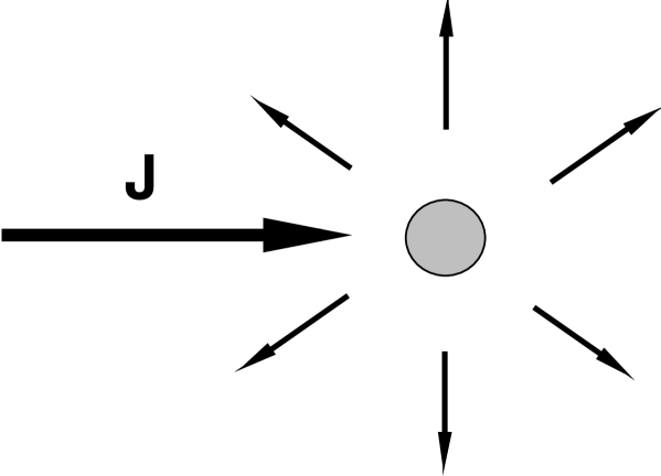
Figure 4: The differential scattering cross section $d\sigma(k,\varphi)$ gives the fraction of an incident current J which is scattered to the angle $\varphi$. In the case of an asymmetric differential scattering cross section there is generally a surplus of particles flowing in one of the transverse directions.

The quantity that measures the fraction of the electrons moving in a transverse direction is $\sin(\varphi)\,d\sigma(k_{F},\varphi)$. Therefore, if the density of vortices is $n_{v}$, the Hall current, in the dilute vortex limit, is proportional to

$$n_{v}\,\int_{-\pi}^{\pi}\!d\varphi\,\sin\varphi\,\frac{d\sigma}{d\varphi}(k_{F},\varphi).$$ (113)

By inverting the conductivity tensor one finds that the Hall resistivity, $\rho_{xy}$, is

$$\rho_{xy}=\rho_{H}^{0}\frac{k_{F}}{\alpha}\int_{-\pi}^{\pi}\!\frac{d\varphi}{2\pi}\sin\varphi\,\frac{d\sigma}{d\varphi}(k_{F},\varphi),$$ (114)

which was obtained by Nielsen and Hedegaard [54]. In the latter case the result (114) was obtained by solving (in the dilute vortex limit) Boltzmann’s equation, which relates the scattering and the transport properties. Here, $\rho_{H}^{0}=Bc/n_{e}e$ is the Hall resistivity in a uniform magnetic field $B$, $n_{e}$ is the density of electrons, and $e$ is the electronic charge. The uniform magnetic field $B$ is obtained by averaging over the field produced by vortices with the density $n_{v}$,

$$B=n_{v}\alpha\Phi_{0}.$$ (115)

Fortunately, because of $\sin\varphi$ factor in Eq. (114), the differential scattering cross section is only needed for $\varphi\neq 0$ to determine the Hall resistivity. When the differential scattering cross section (62) is inserted in Eq. (114) one finds that only the last term contributes and

$$\rho_{xy}=\frac{4n_{v}}{n_{e}}\frac{hc^{2}}{e^{2}}\sin(\pi\alpha)\left[\sin\triangle_{-n}\cos(\triangle_{-n}-\pi\alpha)+\sin\triangle_{-n-1}\cos(\triangle_{-n-1}+\pi\alpha)\right].$$ (116)

Equation (116) shows that one needs more than the asymmetry of the differential scattering cross section for the Hall resistivity to be different from zero. In fact, the Hall resistivity, $\rho_{xy}$, vanishes whenever (modulo $\pi$)

$$\triangle_{-n}=-\triangle_{-n-1}.$$ (117)

However, as has been discussed in Secs. 6 and 7, in any realistic situation relation (117) is not generic and the Hall effect will appear. For example, in the case where the phase-shift flip occurs only in the $l=-n$ channel, i. e., $\triangle_{-n}=\eta\pi$ and $\triangle_{-n-1}=0$, one finds

$$\rho_{xy}=\frac{4n_{v}}{n_{e}}\frac{hc^{2}}{e^{2}}\sin(\pi\alpha)\sin(\eta\pi)\cos(\pi n).$$ (118)

In this case it is easy to check that if the vorticity $\alpha$ increases, $\rho_{xy}$ does not change its sign. Our result (116) shows that the Hall resistivity is proportional to the density of vortices and depends on their vorticity via trigonometrical functions. As a self-consistency check, the Hall resistivity (116) vanishes whenever $\alpha$ is an integer. In the case of vortices in a type II superconductor [10], if the magnetic field increases, the vorticity of each vortex remains constant, and only their density $n_{v}$ changes linearly with the applied field. Therefore, the dependence of the Hall resistivity, $\rho_{xy}$, on the magnetic field is linear in the dilute vortex limit [11]. Obviously, if the magnetic field is sufficiently large, the dilute vortex limit ceases to be valid and deviations appear [10]. Nevertheless, measurements of the Hall effect on a single isolated vortex is now almost experimentally possible [10, 15], and the above results for the Hall resistivity can be tested. Note that, provided the resonance (70) is close to the Fermi energy $E_{F}$, an interesting effect may apear because the Hall resistivity becomes very sensitive to the changes of $E_{F}$.

10 Persistent current of free electrons in the plane pierced by a flux tube

The persistent current in a finite (ring) geometry was first discussed in Ref. [55]. It is reminiscent of the edge currents (see discussion in Ref. [56] on their existence) that arise in the presence of a magnetic field in the absence of the electric force. In the case of a bounded system, the energy levels are discrete and the persistent current induced by a flux tube with flux $\Phi$, carried by the $j$th eigenstate, is [55]

$$i_{j}=-\frac{dE_{j}(\Phi)}{d\Phi}\cdot$$ (119)

In the case of an unbounded system the spectrum will have both a discrete and a continuous part. The persistent current carried by an isolated eigenstate (from a point spectrum) is still given by formula (119). The contribution of scattering states to a persistent current is then determined by the formula

$$dI(E,\alpha)=(2\pi i)^{-1}\partial_{\Phi}\left[\ln\det\mbox{S}(E,\Phi)\right]dE,$$ (120)

derived by Akkermans et al. [6]. Here S$(E,\Phi)$ is the on-shell scattering matrix in the presence of a flux tube, and $dI(E,\Phi)$ is the differential contribution to the persistent current at energy $E$. The persistent current was defined with respect to a point. It was given by the total current through a line that extends from that point to infinity, in the absence of currents through the external leads. Now, by the Krein-Friedel formula (65), $\ln\det\mbox{S}(E,\Phi)$ is directly related to the change $\triangle N_{\alpha}(E)$ of the IDOS, and hence (by using $\Phi=\alpha\Phi_{0}$) we have

$$dI(E,\alpha)=\frac{e}{hc}\,\partial_{\alpha}\left[\triangle N_{\alpha}(E)\right]dE.$$ (121)

As has been shown in Sec. 5, $\triangle N_{\alpha}(E)$ is a symmetric function of $\alpha$. Therefore, a persistent current is an antisymmetric function of $\alpha$ (see Figs. 5 and 6). One can show that the formula (121) reduces to (119) in the case of the discrete spectrum, and in fact, the formula is valid for both continuous and discrete parts of the spectrum. In the latter case, the DOS is formally given by $\rho(E,\Phi)=\sum_{j}\delta[E-E_{j}(\Phi)]$, where the summation is over all discrete levels. Hence

$$\frac{d\rho(E^{\prime},\Phi)}{d\Phi}=-\sum_{j}\delta^{\prime}[E-E_{j}(\Phi)]\,\frac{dE_{j}}{d\Phi}\cdot$$ (122)

Therefore,

$$\int^{E}\frac{d\rho(E^{\prime},\Phi)}{d\Phi}\,dE^{\prime}=-\sum_{j,E_{j}<E}\delta[E-E_{j}(\Phi)]\,\frac{dE_{j}}{d\Phi}\cdot$$ (123)

Now, by substituting the result into Eq. (121) and after integrating up to the Fermi energy $E_{F}$, one recovers the sum over all contributions of single levels, as given by the formula (119), below the Fermi energy $E_{F}$.

For spinless fermions neither bound states nor a phase-shift flip occur and the change in the DOS is given by (22). Therefore, when all states below the Fermi energy $E_{F}$ are occupied, one finds [5] that the persistent current of spinless fermions around the origin, which is pierced by a flux tube, is

$$I=\frac{eE_{F}}{hc}\,(\eta-1/2).$$ (124)

The current depends linearly on $\eta$ (cf. Ref. [6] where it is a constant) as it does in small one-dimensional metal rings [57]. In contrast to Ref. [6], the current is antisymmetric not only about the values $\alpha=n$, where $n$ is an integer, but also about values $\alpha=n+1/2$ where it vanishes (see Fig. 5). The latter values of $\alpha$ are such as the former the values of $\alpha$ where time invariance is preserved.

Figure 5: Characteristic dependence of a persistent current of free spinless fermions in the plane on the flux $\alpha$ (arbitrary units in the $y$ direction).

In the case of spin one-half fermions, the contribution of spin-up fermions to the persistent current is still given by formula (124). The contribution of spin-down fermions depends on their magnetic moment $g_{m}$. At the critical value of $g_{m}=2$, either the phase-shift flip or a bound state can occur. The most general expression for the contribution of scattering states to $\triangle N_{\alpha}(E)$ for $E\geq 0$, which includes the situation where bound states or a phase-sfhift flip are present, is given by Eq. (68). The persistent current in this case is obtained by substituting the result (68) for $\triangle N_{\alpha}(E)$ directly in Eq. (120). Here, one must not forget that the bound state energies also depend on flux [15]. In the case that the phase-shift flip occurs in the $l=-n$ channel, the contribution of spin-down fermions to the persistent current is given by the formula

$$I=\frac{eE_{F}}{hc}\,(\eta+1/2)$$ (125)

[see Fig. 6(a)]. Therefore, the total persistent current of spin one-half fermions in the plane when a phase-shift flip occurs is

$$I=2\frac{eE_{F}}{hc}\,\eta$$ (126)

[see Fig. 6(b)]. This is another important difference from Ref. [6], where they obtained a result that the total current is zero. The result is consistent with general requirements [6] of periodicity with regard to $\alpha\rightarrow\alpha\pm 1$, and antisymmetry with respect to $\alpha\rightarrow-\alpha$.

Figure 6: (a) The contribution of spin-up electrons to the persistent current as a function of the flux $\alpha$, provided that the phase-shift flip occurs in a single channel. (b) Persistent current of spin one-half fermions as a function of the flux $\alpha$.

Provided that the phase-shift flip occurs both in the $l=-n$ and $l=-n-1$ channels, the contribution of spin-down fermions to the persistent current is the same as that of spin-up fermions. However, as has been extensively discussed in Secs. 6 and 7, the latter case of the phase-shift flip in two channels is less probable than that of the phase-shift flip in a single channel.

Observations of the persistent current may finally reveal the resonance (70) in the AB scattering, since near it the current becomes very sensitive to the change of the Fermi energy $E_{F}$ and of the flux. The similarity between the scattering in the presence of the AB potential and in the field of a cosmic string naturally suggests that a similar current should occur in the field of a cosmic string, too.

11 The 2nd virial coefficient of nonrelativistic anyons

Anyons are usually represented as either bosons or fermions threaded by the flux tube with the flux $\Phi$. Noninteracting anyons are described by the Hamiltonian

$$H=\sum_{\stackrel{{\scriptstyle i,j}}{{\scriptscriptstyle i\neq j}}}^{N}\frac{({\bf p}_{i}-\frac{e}{\hbar c}{\bf A}_{ij})^{2}}{2m},$$ (127)

where $N$ is the number of anyons, and ${\bf A}_{ij}={\bf A}({\bf r}_{i}-{\bf r}_{j})$ is nothing but the AB potential (1) centered at the position of the $jth$ particle,

$${\bf A}_{ij}=\frac{\Phi}{2\pi|{\bf r}_{i}-{\bf r}_{j}|^{2}}\,{\bf z}\times({\bf r}_{i}-{\bf r}_{j})=-{\bf A}_{ji},$$ (128)

written here in a slightly different form with ${\bf z}$ the unit vector in the direction of the flux. In what follows we shall consider anyons in the presence of a pairwise interaction $U({\bf r}-{\bf r}^{\prime})$,

$$U({\bf r}-{\bf r}^{\prime})=-\lambda\frac{2\pi\hbar^{2}}{m}\alpha\,\delta^{(2)}({\bf r}-{\bf r}^{\prime})=-\lambda\frac{\hbar^{2}}{m}\frac{\alpha}{|{\bf r}-{\bf r}^{\prime}|}\,\delta(|{\bf r}-{\bf r}^{\prime}|).$$ (129)

By transforming as usual to the center of mass and relative coordinates $(r,\varphi)$, and leaving aside the free motion of the center of mass, the relative Hamiltonian takes the form [7, 46, 58]

$$H_{rel}=-\frac{\hbar^{2}}{m}\left[\partial_{r}^{2}+\frac{1}{r}\partial_{r}-\frac{1}{r^{2}}(-i\partial_{\varphi}+\alpha)^{2}\right]+U({\bf r}-{\bf r}^{\prime}),$$ (130)

where, as above, $\alpha=\Phi/\Phi_{0}$. The form of the relative Hamiltonian $H_{rel}$ corresponds [59] to that used in Refs. [27] and [28]. One neglects the electrostatic forces between anyons by assuming the limit $e\rightarrow 0$ with $\alpha$ fixed. The relative wave function is parametrized as $\exp(iL\varphi)\,f(r)$, where $L$ is standard, namely $L=2l$ for bosons and $2l+1$ for fermions. After parametrization, the relative Hamiltonian $H_{rel}$ takes a form similar to that of $H_{l}$ (4), provided the substitutions $\lambda=g_{m}$ and $s_{z}=-1$ are made, and the reduced mass $\bar{m}=m/2$ is used. Due to the parametrization of the relative wave function, the parameter $\nu$ is now

$$\nu=2l+\alpha$$ (131)

provided one starts from the bosonic end, or

$$\nu=2l+1+\alpha$$ (132)

when one starts from the fermionic end [7, 58].

The equation of state of a real gas expanded in powers of the density, $\mu=N/V$, is

$$PV=\frac{N}{\beta}(1+a_{2}\mu+a_{3}\mu^{2}+\ldots\,)$$ (133)

where the $a_{j}$ stand for the virial coefficients (see, for example, Ref.  [60]). Here, $P$ is the pressure, $V$ is the volume, and $\beta=1/kT$. The calculation of $a_{2}(T)$ only requires a knowledge of two-body interaction. We shall show that the results of preceding sections (with a slight modification) can be directly applied to the calculation of the $2nd$ virial coefficient $a_{2}(T)$ of the gas of anyons. Let us first consider the noninteracting case $\lambda=0$. By using the Krein-Friedel formula one can calculate the change of the DOS in a way similar to that used in Sec. 5. In the case of bosons one finds

$$\ln\det\mbox{S}=\sum_{l=-\infty}^{\infty}2i\delta_{l}=i\pi\sum_{l=-\infty}^{\infty}(|2l|-|2l+\alpha|)$$ (134)

$$=2\pi i\left.\left[\sum_{l=1}^{\infty}l^{-s}-\sum_{l=0}^{\infty}(l+\eta_{a})^{-s}-\sum_{l=1}^{\infty}(l-\eta_{a})^{-s}\right]\right|_{s=-1}$$

$$=2\pi i\left.\left[2\zeta_{R}(s)-\zeta_{H}(s,\eta_{a})-\zeta_{H}(s,1-\eta_{a})\right]\right|_{s=-1}$$

$$=-2\pi i\,\eta_{a}(1-\eta_{a}),$$

and hence

$$\triangle\rho_{\alpha}^{b}(E)=-\eta_{a}(1-\eta_{a})\delta(E).$$ (135)

Now, in the case of anyons, $\eta_{a}$ is the fractional part of $\alpha/2$. Note that formally, if the sum in Eq. (66) is restricted to even $l$ only, the result (135) is twice that in the AB potential with unrestricted $l$. In the case of fermions (here $\eta_{a}$ is supposed to be within the range $|\eta_{a}|<1/2$),

$$\ln\det\mbox{S}=\sum_{l=-\infty}^{\infty}2i\delta_{l}=\pi i\sum_{l=-\infty}^{\infty}(|2l+1|-|2l+1+\alpha|)=$$ (136)

$$=2\pi i\left.\left[\sum_{l=0}^{\infty}(l+1/2)^{-s}+\sum_{l=1}^{\infty}(l-1/2)^{-s}-\sum_{l=0}^{\infty}(l+\eta_{a}+1/2)^{-s}-\sum_{l=1}^{\infty}(l-\eta_{a}-1/2)^{-s}\right]\right|_{s=-1}$$

$$=2\pi i\left.\left[2\zeta_{H}(s,1/2)-\zeta_{H}(s,\eta_{a}+1/2)-\zeta_{H}(s,1/2-\eta_{a})\right]\right|_{s=-1}=2\pi i\,\eta_{a}^{2},$$

and hence

$$\triangle\rho_{\alpha}^{f}(E)=\eta_{a}^{2}\,\delta(E).$$ (137)

Now, the two-body interaction partition function $Z_{int}(\beta)$ can be calculated from

$$Z_{int}^{b,f}(\beta)=\int e^{-\beta E}\,\triangle\rho_{\alpha}^{b,f}(E)\,dE.$$ (138)

Note that $Z_{int}(\beta)$ vanishes for $\eta_{a}=0$ when interactions (including the AB interaction) are switched off. The integration here runs over the whole spectrum. However, since there are no bound states, $\triangle\rho_{\alpha}(E)$ is zero for $E<0$ and the integral reduces to the Laplace transform. By inserting Eqs. (135) and (137) into Eq. (138) one finds that the partition functions do not depend on the temperature $T$ [7],

$$Z_{int}^{b}=-\eta_{a}(1-\eta_{a}),\hskip 28.45274ptZ_{int}^{f}=\eta_{a}^{2}.$$ (139)

$a_{2}(T)$ can be directly expressed in terms of the two-body partition function and has the form

$$a_{2}^{b}(T)=-\frac{\pi\beta}{2m}\left[1+8Z_{int}^{b}\right]$$ (140)

in the case of bosons, and

$$a_{2}^{f}(T)=\frac{\pi\beta}{2m}\left[1-8Z_{int}^{f}\right]$$ (141)

in the case of fermions [7]. The prefactor in the last two expressions can be written as $\lambda_{T}^{2}/4$, where $\lambda_{T}=\sqrt{2\pi\beta/m}$ is the thermal length. Now Eqs. (139), (140), and (141) imply that the $2$nd virial coefficients are periodic with respect to $\eta_{a}\rightarrow\eta_{a}\pm 1$, i. e., with respect to $\alpha\rightarrow\alpha\pm 2$ [27]. In case of bosons one finds for $0<\alpha<2$ that

$$a_{2}^{b}(T)=-\frac{\lambda_{T}^{2}}{4}\left(1-4\alpha+2\alpha^{2}\right)=\frac{\lambda_{T}^{2}}{4}\left[1-2(\alpha-1)^{2}\right].$$ (142)

Similarly, in the case of fermions one obtains for $-1<\alpha<1$ that

$$a_{2}^{f}(T)=\frac{\lambda_{T}^{2}}{4}\left(1-2\alpha^{2}\right)=-\frac{\lambda_{T}^{2}}{4}\left[1-4(\alpha+1)+2(\alpha+1)^{2}\right].$$ (143)

The result for other ranges of $\alpha$ is obtained by using the periodicity. The $2$nd virial coefficients $a_{2}^{b}(T)$ and $a_{2}^{f}(T)$ are written in two equivalent forms. The second form clearly shows that if $\alpha$ is raised to $\alpha+1$, then $a_{2}^{b}(T)\rightarrow a_{2}^{f}(T)$. Similarly, if $\alpha$ is lowered by $1$, then $a_{2}^{f}(T)\rightarrow a_{2}^{b}(T)$.

So far, we have only reproduced the known results for the $2nd$ virial coefficients of noninteracting anyons [7, 27]. In the presence of an interaction (as may be the case for anyon-antianyon interaction) the virial coefficients will change. The results for the DOS in the AB potential then enable us to calculate them in the special case of the potential $U({\bf r}-{\bf r}^{\prime})$. The analysis is similar to that of Sec. 5. Therefore, provided the parameter $\lambda\neq 2$ in Eq. (129), no bound state is present in the spectrum and the $2nd$ virial coefficients $a^{b,f}_{2}(T)$ are still given, respectively, by Eq. (142) or Eq. (143). They exhibit quite a lot of rigidity with respect to the interaction and they start to change only at the critical coupling $\lambda_{c}=2$ when the phase-shift flip or a bound state may occur (at an energy that depends on the details of the limit when the radius of the flux tube shrinks to zero). The only change with regard to the AB scattering discussed in previous sections is that the parameter $\nu$ changes here by $2$ and hence a bound state or the phase-shift flip can only occur in a single channel. Then the change of the IDOS $\triangle N_{\alpha}(E)$ is given either by

$$\triangle N_{\alpha}(E)={\cal N}(\eta_{a})+\frac{1}{\pi}\arctan\left(\frac{\sin(\eta\pi)}{\cos(\eta\pi)-(|E_{-n}|/E)^{\eta}}\right)$$ (144)

or

$$\triangle N_{\alpha}(E)={\cal N}(\eta_{a})-\frac{1}{\pi}\arctan\left(\frac{\sin(\eta\pi)}{\cos(\eta\pi)+(|E_{-n-1}|/E)^{(1-\eta)}}\right),$$ (145)

where either ${\cal N}(\eta_{a})=-\eta_{a}(1-\eta_{a})$ or ${\cal N}(\eta_{a})=\eta_{a}^{2}$ depending on $n$ and whether one starts from the bosonic or the fermionic end. To calculate $Z_{int}(\beta)$ in this case one integrates by parts the general formula (138) and rewrites it in terms of the change $\triangle N_{\alpha}(E)$ of the IDOS [61]. Now a bound state is present and one obtains in general

$$Z_{int}(\beta)=\sum_{b}e^{-\beta E_{b}}+\beta\int_{0}^{\infty}e^{-\beta E}\triangle N_{\alpha}(E)\,dE,$$ (146)

where the sum here in principle runs over all bound states. Note that at the critical coupling, the partition function depends on $T$. Eventually, the $2nd$ virial coefficients are obtained by inserting the result in either (142) or (143). In Table I the results are presented for the partition function, and the $2$nd virial coefficient for bosons and fermions in the case when the phase-shift flip occurs for $n=[\alpha]$ irrespective of whether odd ($n=n_{o}$) and even ($n=n_{e}$). The results are presented in terms of $\eta$. Provided $n$ is even, $\eta$ is added to (subtracted from) $Z_{int}(\beta)$ in the case of bosons (fermions). The reason is that in the former case the condition $0<|\nu|<1$ is satisfied for the only $l$ given by $2l=-n$ ($2l=-n-2$), which implies that the parameter $\nu$ takes the value $\eta$ [$-(1-\eta)$]. When $n$ is odd, the situation is reversed and $\eta$ is subtracted from (added to) $Z_{int}(\beta)$ in the case of bosons (fermions). The calculation can be performed straightforwardly, but care has to be taken with regard to the range of $\eta_{a}$: $0<\eta_{a}<1$ in the case of bosons and $|\eta_{a}|<1/2$ in the case of fermions.

TABLE I. The partition function $Z_{int}(\beta)$ and the $2$nd virial coefficient for bosons and fermions in the presence of the phase-shift flip for $n=[\alpha]$ odd and even.

n	$Z^{b}_{int}(\beta)$	$a_{2}^{b}(T)$	$Z^{f}_{int}(\beta)$	$a_{2}^{f}(T)$
even	$\frac{1}{4}(2\eta+\eta^{2})$	$\frac{\lambda_{T}^{2}}{4}\left[1-2(\eta+1)^{2}\right]$	$\frac{1}{4}(-4\eta+\eta^{2})$	$\frac{\lambda_{T}^{2}}{4}\left(1+8\eta-2\eta^{2}\right)$
odd	$-\frac{1}{4}(1+4\eta-\eta^{2})$	$\frac{\lambda_{T}^{2}}{4}\left(1+8\eta-2\eta^{2}\right)$	$\frac{1}{4}(\eta+1)^{2}$	$\frac{\lambda_{T}^{2}}{4}\left[1-2(\eta+1)^{2}\right]$

The results presented in Table I, apart from the periodicity of the $2$nd virial coefficients, demonstrate clearly that the $2$nd virial coefficients interpolate between the fermionic and bosonic case as $\alpha$ changes by unity. Namely, the $2$nd virial coefficient in the $n_{o}B$ case (bosonic end with $n=n_{o}$ odd) is the same as that in the $n_{e}F$ case (fermionic end with $n=n_{e}$ even), and similarly the result for the $2$nd virial coefficient in the $n_{o}F$ case is the same as that in the $n_{e}B$ case. The reason is that in the respective cases, the partition functions $Z^{b,f}_{int}$ receive the same contribution. This is not restricted to the case when the contribution is given by the phase-shift flip only, but holds in the general case [(145) and (146)] when the bound state is present. Then, according to Eqs. (140) and (141), the changes in the $2$nd virial coefficients are identical. Therefore, the interpolation between different statistics as $\alpha\rightarrow\alpha\pm 1$ holds both with and without the short-range interaction (129). There is, however, one distinguishing feature of the $2$nd virial coefficients at the critical coupling observed in Ref. [28], namely, their discontinuity. Since a discontinuity in the virial coefficient implies a discontinuity in the free energy, to the same order of approximation this points to some kind of phase transition [28]. It has already been mentioned that at the critical coupling $\lambda_{c}=2$, the scale invariance is generally broken and one expects a different physics in this case.

Our results cover naturally the case of the spin one-half anyons [28], too. In the latter if we ignore the anomalous part of the magnetic moment, but add a Zeeman interaction, an anyon-anyon potential $U({\bf r}-{\bf r}^{\prime})$ arises which has the form

$$U({\bf r}-{\bf r}^{\prime})=\frac{\hbar^{2}}{m}(s_{1}+s_{2})\frac{\alpha}{|{\bf r}-{\bf r}^{\prime}|}\,\delta(|{\bf r}-{\bf r}^{\prime}|),$$ (147)

where $s_{1}=\pm 1$ and $s_{2}=\pm 1$ are spin projections on the direction of the flux tube [28]. Provided that at least one of the spins does not have an orientation opposite to the orientation of the magnetic field, then, depending on the statistics, the result for the $2$nd virial coefficient is given either by Eq. (142) or Eq. (143), in accord with [28] and with previous results [7, 27]: the interaction does not have its critical value and one should recover the noninteracting case. If both spins are opposite to the direction of the magnetic field, the critical potential with $\lambda_{c}=2$ arises and, provided the phase-shift flip takes the place, the results for the $2$nd virial coefficient of anyons can be read off from Table I. Our result in the $n_{o}F$ case agrees with that of Blum et al. [28]. In the $n_{e}F$ case they did not take into account that the phase-shift flip may occur as they assumed that in the AB scattering the phase-shift flip cannot occur in the $l\!=\!-n-1$ channel. Therefore, not surprisingly, in the absence of the phase-shift flip in Ref. [28] they obtained the same result (143) for the $2$nd virial coefficient in the $n_{e}F$ case as in the absence of the interaction $U({\bf r}-{\bf r}^{\prime})$. As has been discussed in Sec. 6, it is more difficult to create a bound state in the $l=-n-1$ channel, and the phase-shift flip in this channel may possibly not occur. If this happens, then our result for the $2$nd virial coefficient coincides with that of Ref. [28].

For the case of an unpolarized system, the complete $\bar{a}_{2}^{f}(T)$ is obtained by averaging over four spin states. Provided that there is no phase-shift flip in the $n_{e}F$ case, $a_{2}^{f}(T)$ is the same in all four cases and is given by Eq. (143). In the presence of the phase-shift flip, one of the values $a_{2}^{f}(T)$ is then given by Table I. In the $n_{o}F$ case, three values of $a_{2}^{f}(T)$ are the same and given by Eq. (142), because of the interpolation between fermionic and bosonic statistics. The remaining value of $a_{2}^{f}(T)$ under the presence of the phase-shift flip is again taken from Table I. Finally, one obtains

$$\bar{a}^{f}_{2}(T)=\frac{\lambda_{T}^{2}}{4}\left\{\begin{array}[]{ll}(1-2\eta^{2}),&\ n_{e}F\ \mbox{case without the phase-shift flip}\\ (1+2\eta-2\eta^{2}),&\ n_{e}F\ \mbox{case with the phase-shift flip}\\ (-1+2\eta-2\eta^{2}),&\ n_{o}F\ \mbox{case}.\end{array}\right.$$ (148)

It is worth noting that anyons with a short-range pairwise attractive interaction occur in the nonrelativistic limit, taken up to the terms of order $v^{2}/c^{2}$, of the topologically massive planar electrodynamics [51] defined by the action

$$S=S_{matter}+$$ (149)

$$\frac{1}{L^{2}}\int\left(-\frac{1}{4}F_{\alpha\beta}F^{\alpha\beta}+\frac{1}{2R}\epsilon_{\alpha\beta\gamma}A^{\alpha}\partial^{\beta}A^{\gamma}\right)dt\,d^{2}{\bf r},$$

with a nonminimal coupling [25, 26]

$$S_{matter}=S^{0}_{matter}-$$ (150)

$$\sum_{a=1}^{N}\int J^{\mu}_{(a)}(x)\left[\xi_{a}A_{\mu}(x)-\frac{1}{2}g_{a}L^{-2}\epsilon_{\mu\nu\sigma}F^{\nu\sigma}\right]dt\,d^{2}{\bf r}.$$

Here, $|R|$ represents the screening length of the electromagnetic interaction, $L$ is the arbitrary scale parameter, $\xi_{a}$ stands for the $a$th particle’s charge in units of $L$, $J^{\mu}_{(a)}$ denotes the standard one-particle current normalized to the unit charge, and $N$ is the number of the pointlike particles. In the model the photon is massive with a mass $M=\hbar/c|R|$. Note that $F^{12}$ is actually a magnetic field, and the nonminimal coupling term that is peculiar to $2+1$ dimensions [25, 26] is in this instance the familiar Pauli magnetic moment coupling that exists here even in the absence of a spin. It has been shown by Stern [25] that, provided

$$g_{a}=L^{2}R\,\xi_{a},$$ (151)

$\oint_{C}dx^{i}A_{i}$ becomes a topological invariant,

$$\oint_{C}dx^{i}A_{i}=gn.$$ (152)

The screening length remains nonzero, and the electric charge and magnetic moment balance each other in such a way that the radiation is absent. At the tree level, the theory at the critical coupling (151) can be exactly reexpressed as a simple effective action at a distance without the usual complications associated with the retardation, etc. [25]. The situation is analogous to that in pure Chern-Simons (CS) theory,

$$S_{CS}=\frac{1}{2\Theta}\int\epsilon_{\alpha\beta\gamma}A^{\alpha}\partial^{\beta}A^{\gamma}dt\,d^{2}{\bf r}$$ (153)

which is recovered in the limit $L^{2}\rightarrow\infty$, $R\rightarrow 0$, keeping fixed the parameter

$$\Theta=L^{2}R.$$ (154)

In the latter case the absence of radiation is simply because the photon gets infinitely heavy. At the tree level, the theory at the critical coupling (151) can be exactly reexpressed as a simple effective action at a distance without the usual complications associated with the retardation, etc. [25].

12 Discussion of the results and open questions

The nonrelativistic scattering in the AB potential has been analyzed. The DOS and scattering cross sections have been calculated and various applications have been discussed. Despite the fact that the single-particle Green function is not a periodic function of $\alpha$, it gives rise to the DOS which is a periodic and symmetric function of the flux and it depends only on the distance from the nearest integer. It has been shown that the Krein-Friedel formula [8] is not restricted to potentials of a finite range and can have a wider range of applicability. The Krein-Friedel formula may be used even for long-ranged potentials when the sum over phase shifts is properly regularized. In the case of the Aharonov-Bohm potential it is the $\zeta$-function regularization that gives the correct answer. By means of the Krein-Friedel formula the change of the DOS induced by the Aharonov-Bohm potential has been calculated for different self-adjoint extensions which correspond to different physics inside the flux tube. For the conventional setup, i. e., with zero boundary conditions at the boundary of the flux tube, our result for the DOS (22) confirms the anticipation of Comtet, Georgelin, and Ouvry [7] that the change of the DOS is concentrated at the zero energy. Whenever a bound state is present it is always accompanied by a resonance at an energy proportional to the absolute value of the energy of the bound state. In the presence of a bound state or a phase-shift flip, the symmetry of the spectrum with respect to the change $\alpha\rightarrow\alpha\pm 1$ is broken. Nevertheless, scattering cross sections continue to be periodic with respect to the substitution $\alpha\rightarrow\alpha\pm 1$.

In the case of a regular flux tube of a finite radius $R$, the question of the number of bound states has been clarified. It has been shown that the number depends not only on the total flux but also on the energy of magnetic field. It means that one has to be careful in the choice of the regularization when discussing the physics with anomalous magnetic moment $g_{m}\geq 2$ or with a short-range interaction inside the flux tube. When the AB vortex arises by some physical mechanism such as vortices in the superconductor of type II do, then the profile of a magnetic field is determined by the condition of the minimum of energy. Our considerations have only been quantitative. The open question which remains is what is the qualitative dependence on the energy and whether (and if then, how) the number of bound states depends on higher moments $\int B^{n}(r)\,d^{2}\,{\bf r}$ of the magnetic field $B(r)$, where $n\geq 3$. We have shown that a bound state in the $l\!=\!-n-1$ channel can exist provided $1-\eta$ is sufficiently small. In the discussion of the $R\rightarrow 0$ limit, the existence of a critical coupling $g_{m}=2$ was established. Provided the coupling with the interior of the flux tube is smaller or greater than the critical one, or when the coupling is not renormalized, the limit coincides with that of the impenetrable flux tube. Thereby, the result of Ref. [49] for $g_{m}=0$ is generalized. The Aharonov-Casher theorem about the number of zero modes has been corrected. It has been shown that they merge with the continuous spectrum in the $R\rightarrow 0$ limit. The origin of the phase-shift flip has been investigated. It was shown that the phase-shift flip [14] may occur even in the absence of spin. The conditions for the phase-shift flip formulated in Refs. [14, 22] have been found necessary but not sufficient. In particular, provided no bound state is in the $l\!=\!-n-1$ channel for $R\neq 0$, then the phase-shift flip will not occur at the $R\rightarrow 0$ limit.

A quantum-mechanical and nonrelativistic criterion of stability (112) in $2+1$ dimensions has been discussed that only involves fundamental parameters of matter. Despite that this criterion was derived under very restrictive hypotheses, it was shown to be compatible with other, quantum-field theory treatments [52, 53]. An open question remains regarding what will happen if the dynamics of the shrinking of the radius of a flux tube is included. Another open question is what field configuration actually optimalizes the right-hand side of Eq. (112), i. e., what is the infimum of the right-hand side of Eq. (112) with respect to variations of magnetic field $B(r)$, subject to the constraint (87).

It has been shown that in the presence of bound states or a phase-shift flip, the differential scattering cross section becomes asymmetric with respect to the substitution $\varphi\rightarrow-\varphi$, and gives rise to the Hall effect. The Hall resistivity has been calculated [see Eq. (116)]. The persistent current of free electrons in the plane has been discussed and the results of Ref. [6] have been extended. In contrast to Ref. [6], we have found that the total persistent current in the spin one-half case is different from zero, and the persistent current of both the spinless and the spin one-half fermions depends linearly on $\eta$. The formal similarity between the scattering of electrons in the AB potential and that in the field of a cosmic string suggests that a persistent current will also appear in the latter case.

The known results for the $2nd$ virial coefficients of the nonrelativistic anyons [7, 27] were reproduced and their values were calculated for the case when anyons interact via a short-range attractive potential, $U({\bf r}-{\bf r}^{\prime})$, proportional to the Dirac $\delta$ function given by Eq. (129). The case considered here is complementary to the case of a long-range potential $g/r^{2}$, considered by Loss and Fu [62]. In the present case, the $2nd$ virial coefficients were shown to be remarkably stable when such an interaction is switched-on. They do not change when the interaction is switched on until the coupling constant reaches its critical strength. At the critical coupling the $2$nd virial coefficients become discontinuous as a function of $\alpha$ but their periodicity with respect to $\alpha\rightarrow\alpha\pm 2$ and the interpolation $a_{2}^{b,f}(\alpha\pm 1)=a_{2}^{f,b}(\alpha)$ between different statistics still hold. These results were obtained by using the $\zeta$-function regularization which has an obvious advantage with regard to other finite box or harmonic potential regularizations. By using the $\zeta$-function regularization one avoids the necessity of a discretization of energy levels for computing the partition function. Our results naturally generalize those of Blum et al. [28] for nonrelativistic spin one-half anyons for the case of an anomalous magnetic moment and when a bound state occurs in the spectrum.

Our results have been formulated in terms of self-adjoint extensions. A self-adjoint extension is the rigorous limit $R\rightarrow 0$. Therefore, in the case of a flux tube of finite radius $R$, our results can be applied when the radius $R$ is negligibly small when compared to all other length scales in the system under consideration. The parameters $\triangle_{-n}$ and $\triangle_{-n-1}$ of the relevant self-adjoint extension are then determined from bound state energies in the $l=-n$ and $l=-n-1$ channels. Hence, to check some of our results experimentally it is not necessary to use a singular magnetic field. By using the duality discussed in Sec. 7 the physics in the presence of an almost singular flux tube can be tested in experiments with slow electrons scattered off a general rotationally invariant two-dimensional magnetic field $B(x,y)$ that obeys the finite-flux condition (87). From the experimental point of view we stress the following experiments that should be performed:

• Measurement of the phase shift flip in the $l\!=\!-n-1$ channel. Depending on the flux it may or may not occur in this channel.

• Measurements of the Hall resistivity either in the dilute vortex limit or for the single vortex.

• Measurements of the resonance.

A hypothetical setup to observe the resonance is to study the transmission through a single flux tube. A realistic physical realization is that suggested originally by Rammer and Shelankov [11] and later realized experimentally by Bending, Klitzing, and Ploog [10] (see Fig. 1). When homogeneous magnetic field is switched on, the conventional superconductor is penetrated by vortices of flux with $\alpha=1/2$, i. e., exactly that flux at which the resonance is at infinity. Recent measurements on YBCO-delta rings with three grain-boundary Josephson junction [63], however, reported the observation of vortices that carry a flux $\alpha=1/4$ which is smaller than the standard flux quantum $hc/2e$ (corresponding to $\alpha=1/2$) in the superconductor. Therefore, when the high-T_c YBCO film is used as a gate on top of the heterostructure containing 2DEG, the resonance is at some finite energy and could in principle be observed. Another possibility is to measure energy dependence of phase shifts and (as a precursor of the resonance) the time delay (74).

An interesting open problem concerns the shape of the resonance (71) in the AB scattering that is not of the Breit-Wigner form. The latter is a general consequence of the analyticity of scattering amplitudes that is usually taken as an equivalent to causality. However, the rigorous proof of the equivalence requires precise localization in time and in the energy for the incident wave packet. This is, however, impossible due to the uncertainity relations impossible [64]. We have undertaken the analysis of the problem in terms of the Jost functions. However, we have not found the origin of this behavior and we postpone the solution to this problem. The discussion might in principle shed some light on the analyticity principle usually adopted in the axiomatic quantum-field theory as a substitute for causality.

Another interesting problem is to find the analog of the Levinson theorem (see Ref. [41], p. 356, and Ref. [65]) and the generalization of Bargmann’s inequalities [66] for singular potentials. In the case of regular potentials of finite range one knows, thanks to this theorem, that if the phase shifts are normalized so that $\delta_{l}(E)=0$ for $E\rightarrow\infty$, then $\delta_{l}(0)$ gives the number of bound states in the channel $l$. In the case of the AB potential the phase shifts (7) essentially do not depend on the angular momentum $l$ and on the energy $E$. In the case of $\alpha<1$ they are either $-\pi\alpha$ for positive $l$ or $\pi\alpha$ for negative $l$. It is impossible in general to normalize phase shifts in the singular case in the same way as for regular potentials, since they do not depend on the energy.

13 Acknowledgments

I should like to thank IPN at Orsay for warm hospitality during my stay there and, in particular, A. Comtet, Y. Georgelin, M. Knecht, S. Ouvry, and J. Stern for suggestions on literature and many useful and stimulating discussions, and Mme. C. Paulin for drawing the figures. Partial support by the UK EPSRC Grant GR/J35214 and by the Grant Agency of the Czech Republic under Project No. 202/93/0689 are also gratefully acknowledged. Last but not least I thank R. C. Jones for careful reading of the manuscript.

Appendix A Some useful integrals

To perform the integral in Eq. (14) one uses the result that

$$J_{\nu}(kr_{y})=\frac{1}{2}\left[H^{(1)}_{\nu}(kr_{y})+H^{(2)}_{\nu}(kr_{y})\right]$$ (155)

and deforms the integration contour as in Fig. 2. $H^{(1)}$ and $H^{(2)}(z)$ are the Hankel functions,

$$H^{(1)}(z)=\frac{i}{\sin\nu\pi}\left[e^{-\nu\pi i}J_{\nu}(z)-J_{-\nu}(z)\right].$$ (156)

For real arguments,

$$H^{(1)}(x)=H^{(2)}(x)^{*}$$ (157)

[see Ref.  [34], relations (9.1.3) and (9.1.4)]. The integral with $H^{(1)}_{\nu}(kr_{y})$ is now deformed to the contour $C_{1}$ while that with $H^{(2)}_{\nu}(kr_{y})$ is deformed to the contour $C_{2}$. Note that $H^{(1)}_{\nu}(z)$ [$H^{(2)}_{\nu}(z)$] is exponentially decreasing in the upper (lower) half of the complex plane (see Appendix B). Since it is assumed that $r_{x}<r_{y}$ the integrand in Eq. (14) is exponentially decreasing as well. Now, the contributions of any of the two integrals from the imaginary axis do not vanish. However, by using the identities (9.1.35) and (9.1.39) from Ref.  [34],

$$J_{\nu}(ze^{\pm\pi i})=e^{\pm\nu\pi i}J_{\nu}(z),$$ (158)

$$H^{(2)}_{\nu}(ze^{-\pi i})=-e^{\nu\pi i}H^{(1)}_{\nu}(z),$$ (159)

$$H^{(1)}_{\nu}(ze^{\pi i})=-e^{-\nu\pi i}H^{(2)}_{\nu}(z),$$ (160)

one can show that

$$\int_{i\infty}^{0}\frac{zdz}{q^{2}-z^{2}}J_{\nu}(zr_{x})H^{(1)}_{\nu}(zr_{y})=-\int_{-i\infty}^{0}\frac{zdz}{q^{2}-z^{2}}J_{\nu}(zr_{x})H^{(2)}_{\nu}(zr_{y}),$$ (161)

i. e., the integrals on the imaginary axis cancel in the sum. Thanks to (159) one has for $\nu=0$

$$H^{(2)}_{0}(ze^{-\pi i})=-H^{(1)}_{0}(z),$$ (162)

and the same applies to the integral in Eq. (12), too. Once the integrals in Eqs. (12) and (14) are represented as the sum of two contour integrals in the complex plane they can be simply taken by the residue theorem.

In order to calculate $\mbox{Tr}\,\triangle G_{\alpha}({\bf x},{\bf x},M)$ note that

$$\mbox{Tr}\,\triangle G_{\alpha}({\bf x},{\bf x},M)=\int_{R^{2}}\triangle G_{\alpha}({\bf x},{\bf x},M)\,d^{2}{\bf x}=$$ (163)

$$-\frac{\sin\eta\pi}{2\pi M^{2}}\int_{-\infty}^{\infty}d\vartheta\,\int_{-\infty}^{\infty}d\omega\frac{1}{(\cosh\omega+\cosh\vartheta)^{2}}\,\frac{e^{\eta(\vartheta-\omega)}}{1+e^{\vartheta-\omega}},$$

To perform the integral here one makes the substitution [67]

$$x=\frac{\vartheta+\omega}{2},\hskip 28.45274pty=\frac{\vartheta-\omega}{2},$$ (164)

with a Jacobian equal to $2$. After some manipulations one finds

$$\int_{-\infty}^{\infty}d\vartheta\,\int_{-\infty}^{\infty}d\omega\frac{1}{(\cosh\omega+\cosh\vartheta)^{2}}\,\frac{e^{\eta(\vartheta-\omega)}}{1+e^{\vartheta-\omega}}=$$ (165)

$$\int_{0}^{\infty}\frac{dx}{\cosh^{2}x}\int_{0}^{\infty}\frac{\cosh(2\eta-1)y}{\cosh^{3}y}dy.$$

According to formula (3.512.1) of Ref. [36]

$$\int_{0}^{\infty}\frac{\cosh(2\eta-1)y}{\cosh^{3}y}dy=2B(1+\eta,2-\eta),$$ (166)

where $B(x,y)$ is the Euler beta function,

$$B(x,y):=\frac{\Gamma(x)\Gamma(y)}{\Gamma(x+y)},$$ (167)

and $\Gamma(x)$ is the Euler gamma function [34, 36]. Since $B(1,1)=1$,

$$\int_{0}^{\infty}\frac{1}{\cosh^{2}x}\,dx=1.$$ (168)

Now, $\Gamma(3)=2$ and

$$2B(1+\eta,2-\eta)=\Gamma(1+\eta)\Gamma(2-\eta)=$$ (169)

$$\eta(1-\eta)\Gamma(\eta)\Gamma(1-\eta).$$

Therefore, by using (176),

$$\int_{0}^{\infty}\frac{\cosh(2\eta-1)y}{\cosh^{3}y}\,dy=\pi\frac{\eta(1-\eta)}{\sin\pi\eta}\cdot$$ (170)

Appendix B Cylindrical functions and the exterior solution

The asymptotic behavior of Bessel functions and their derivatives at infinity as $z\rightarrow\infty$ can be found directly in Ref. [34]. The asymptotic behavior of the Bessel function $J_{\nu}(z)$ and their derivatives at the origin as $z\rightarrow 0$ is determined by relation (9.1.10) of Ref. [34]. The asymptotic behavior of the Hankel function at the origin for $|\nu|<1$ can be calculated from the asymptotic behavior of $J_{\nu}(z)$ by using relation (9.1.3) of Ref. [34],

$$H^{(1)}_{\nu}(z) = \frac{1}{i\sin\nu\pi}\sum_{m=0}^{\infty}\frac{(-z^{2}/4)^{m}}{m!}\left[\frac{(z/2)^{-\nu}}{\Gamma(1-\nu+m)}-e^{-\nu\pi i}\,\frac{(z/2)^{\nu}}{\Gamma(1+\nu+m)}\right],$$ (171)

$$H^{(1)}_{0}(z) = 1-\frac{2}{\pi i}\left[\ln\left(\frac{z}{2}\right)+\gamma\right]+{\cal O}(z^{2}\ln z),$$ (172)

where $\gamma$ is Euler’s constant. The asymptotic behavior of $K_{\nu}(z)$ for $\nu<1$ when $z\rightarrow 0$ is determined with the help of the last two formulas and relations (9.6.4) and (9.6.6) of Ref. [34], that hold for $-\pi<\arg\,z\leq\pi/2$. Therefore,

$$K_{0}(z)\sim-\gamma-\ln(z/2)+{\cal O}(z^{2}\ln z),$$ (173)

and

$$K_{\nu}(z) \sim \frac{1}{2\sin\nu\pi}\frac{\pi}{\Gamma(1-\nu)}\left[\left(\frac{z}{2}\right)^{-\nu}-\frac{\Gamma(1-\nu)}{\Gamma(1+\nu)}\left(\frac{z}{2}\right)^{\nu}\right]+{\cal O}(z^{2-\nu})$$ (174)

$$= \frac{1}{2}\Gamma(\nu)\left[\left(\frac{z}{2}\right)^{-\nu}-\frac{\Gamma(1-\nu)}{\Gamma(1+\nu)}\left(\frac{z}{2}\right)^{\nu}\right]+{\cal O}(z^{2-\nu}),$$

$$K_{\nu}^{\prime}(z)=-\frac{1}{4}\Gamma(1+\nu)\left[\left(\frac{z}{2}\right)^{-\nu-1}+\frac{\Gamma(1-\nu)}{\Gamma(1+\nu)}\left(\frac{z}{2}\right)^{\nu-1}\right]+{\cal O}(z^{1-\nu}),$$ (175)

otherwise. Here we have used the identity $\nu\Gamma(\nu)=\Gamma(1+\nu)$ together with

$$\Gamma(\nu)\Gamma(1-\nu)=\frac{\pi}{\sin\nu\pi}\cdot$$ (176)

The wave function outside the flux tube is

$$\psi_{l}(r,\varphi)=K_{|l+\alpha|}(\kappa_{l}r)e^{il\varphi}.$$ (177)

For its logarithmic derivative $rK_{\nu}^{\prime}(r)/K_{\nu}(r)$ one has in general (see formula 9.6.26 of Ref.  [34])

$$z\frac{K_{\nu}^{\prime}(z)}{K_{\nu}(z)}=-\nu-z\frac{K_{\nu-1}(z)}{K_{\nu}(z)}=\nu-z\frac{K_{\nu+1}(z)}{K_{\nu}(z)}\cdot$$ (178)

Its asymptotic behavior as $z\rightarrow 0$ depends whether $\nu$ is less than, equal to, or greater than $1$. One has

$$z\frac{K_{\nu}^{\prime}(z)}{K_{\nu}(z)}\sim-\nu-2\nu\frac{\Gamma(1-\nu)}{\Gamma(1+\nu)}\,\left(\frac{z}{2}\right)^{2\nu}+{\cal O}(z^{4\nu})$$ (179)

for $0<\nu<1/2$,

$$z\frac{K_{\nu}^{\prime}(z)}{K_{\nu}(z)}\sim-\nu-2\nu\frac{\Gamma(1-\nu)}{\Gamma(1+\nu)}\,\left(\frac{z}{2}\right)^{2\nu}+{\cal O}(z^{2})$$ (180)

for $1/2\leq\nu<1$,

$$z\frac{K_{\nu}^{\prime}(z)}{K_{\nu}(z)}\sim-1+\frac{1}{\Gamma(2)}z^{2}\ln z+{\cal O}(z^{2})$$ (181)

for $\nu=1$, and

$$z\frac{K_{\nu}^{\prime}(z)}{K_{\nu}(z)}\sim-\nu-\frac{1}{2(\nu-1)}z^{2}+{\cal O}(z^{2\nu},\,z^{4})$$ (182)

for $\nu>1$. At infinity as $r\rightarrow\infty$

$$r\frac{K_{\nu}^{\prime}(r)}{K_{\nu}(r)}\sim-r-\frac{1}{2}+{\cal O}(r^{-1}).$$ (183)

Appendix C Hypergeometric function and the interior solution

In the case of homogeneous field regularization, the wave function inside the flux tube of radius $R$ at the energy $E$ is given by (cf. Ref. [43], p. 458)

$$\psi({\bf r})=e^{-\xi/2}\xi^{|l|/2}\hskip 56.9055pt$$ (184)

$$M\left(\frac{|l|+l}{2}-\frac{\varepsilon(r)}{2}-\frac{1}{2}\,k^{2}l_{B}^{2},|l|+1,\xi\right)e^{il\varphi}.$$

Here $\xi$ is the flux within the radius $r$ in units of the flux quantum $\Phi_{0}$, $\xi=l^{2}_{B}r^{2}/2=\Phi(r)/\Phi_{0}$, $l_{B}=(\hbar c/|e|B)^{1/2}$ is the magnetic length, $k^{2}=2mE/\hbar^{2}$, and the magnetic moment coupling has been assumed inside the flux tube. Since we are interested in bound states, the parameter $x=\kappa R$ will be introduced in analogy with Ref. [39] where, as above, $\kappa=\sqrt{2m|E_{b}|}/\hbar^{2}$, $E_{b}$ being the bound state energy. One can show that

$$\frac{x^{2}}{2\alpha}=-\frac{2mE_{b}}{\hbar^{2}}l_{B}^{2}.$$ (185)

The logarithmic derivative of (184) at the flux tube radius $r=R$ is then

$$\left.r\frac{\psi({\bf r})^{\prime}}{\psi({\bf r})}\right|_{r=R}=-\alpha+|l|+2\alpha\frac{a}{b}\,\frac{M\left(a+1,b+1,\alpha\right)}{M\left(a,b,\alpha\right)},$$ (186)

where $a$ and $b$ are given by Eq. (85).

The Kummer function $M(a,b,z)$, frequently denoted by ${}_{1}F_{1}(a,b,z)$ [34], is defined by

$$M(a,b,z)=1+\frac{a}{b}z+\frac{a(a+1)}{b(b+1)}\frac{z^{2}}{2!}+\ldots+\frac{a_{n}}{b_{n}}\frac{z^{n}}{n!}+\ldots.$$ (187)

where

$$a_{n} = a(a+1)\ldots(a+n-1),$$

$$b_{n} = b(b+1)\ldots(b+n-1).$$ (188)

Due to the formula 13.4.8 of Ref. [34]

$$\frac{d}{dz}M(a,b,z)=\frac{a}{b}M(a+1,b+1,z).$$ (189)

Using the simple fact that, provided $b>0$,

$$a\,<\,b\hskip 14.22636pt\Longrightarrow\hskip 14.22636pt\frac{a}{b}\,<\,\frac{a+1}{b+1},$$ (190)

one finds for real $z=c>0$

$$M(a,b,c)<M(a+1,b+1,c).$$ (191)

Note that in the cases discussed here [see Eqs. (79) and (85)] one has not only $b>0$ but even $b\geq 1$. Moreover, provided there is neither magnetic moment coupling nor an attractive potential inside the flux tube one also has $a>0$ [see Eq. (79)], and Eq. (80) holds. However, one cannot maintain

$$M(a,b,c)>0$$ (192)

when an attractive potential of whatever origin is inside the flux tube. For example, for $g_{m}-2=2\varepsilon<4$ and $x\in\left[0,\sqrt{2\alpha\varepsilon}\,\right)$ [see Eq. (85)] one has $-1<a<0$. In this case $a+1>0$ and $M(a+1,b+1,c)>0$. From the definition (187) of $M(a,b,c)$ one finds easily for such $a$ that

$$M(-|a|,b,c)=2-M(|a|,b,c).$$ (193)

Therefore, if the relation

$$M(|a|,b,c)>2$$ (194)

is satisfied, one finds $M(a,b,c)<0$. Hence,

$$\frac{M(a+1,b+1,c)}{M(a,b,c)}<0.$$ (195)

The ratio at $x=0$ is nothing but a parameter $\alpha_{1}$ of Ref. [39]. It is here where the error [45] in Ref. [39] is made since they claimed $\alpha_{1}$ to be positive for whatever are the parameters $a$, $b$, and $c$. For our purposes it is more important to discuss the property of the ratio given in Eq. (80) in place of (195). Note that the ratio stays positive,

$$\frac{2a}{b}\,\frac{M(a+1,b+1,\alpha)}{M(a,b,\alpha)}>0,$$ (196)

provided Eq. (194) holds. Therefore, at those values of $x$ [it enters Eq. (194) via $a$] it is impossible to satisfy Eq. (82) with the homogeneous field regularization.

Appendix D $\zeta$ functions

The Riemann $\zeta$ function is defined by

$$\zeta_{R}(s):=\sum_{l=1}^{\infty}l^{-s}.$$ (197)

It is an analytic function with a simple pole at $s=1$. The Hurwitz $\zeta_{H}(s,x)$ function, $x\not\in Z$, is a generalization of $\zeta_{R}(s)$,

$$\zeta_{H}(s,x):=\sum_{l=0}^{\infty}(l+x)^{-s}.$$ (198)

For $s=-1$

$$\zeta_{R}(-1)=-\frac{1}{12},$$ (199)

and

$$\zeta_{H}(-1,x)=\frac{1}{2}x(1-x)-\frac{1}{12}=\frac{1}{2}x(1-x)+\zeta_{R}(-1).$$ (200)

References

- [1] W. Ehrenberg and R. E. Siday, Proc. Phys. Soc. 62B, 8 (1949); Y. Aharonov and D. Bohm, Phys. Rev. 115, 485 (1959); W. C. Henneberger, Phys. Rev. A 22, 1383 (1980).
- [2] M. Alford and F. Wilczek, Phys. Rev. Lett. 62, 1071 (1989).
- [3] A. J. Niemi and G. W. Semenoff, Phys. Rev. Lett. 51, 2077 (1983); T. Jaroszewicz, Phys. Rev. D 34, 3128 (1986).
- [4] A. Moroz, Report IPNO-TH/ 94-20 (hep-th/9404104); Phys. Lett. B 358, 305 (1995); Report IPNO/TH 94-89; Mod. Phys. Lett. B9, 1407 (1995); Report TPBU-2-95 (hep-th/9511121).
- [5] A. Comtet, A. Moroz, and S. Ouvry, Phys. Rev. Lett. 74, 828 (1995).
- [6] E. Akkermans, A. Auerbach, J. E. Avron, and B. Shapiro, Phys. Rev. Lett. 66, 76 (1991).
- [7] A. Comtet, Y. Georgelin, and S. Ouvry, J. Phys. A: Math. Gen. 22, 3917 (1989).
- [8] J. M. Lifschitz, Usp. Matem. Nauk 7, 170 (1952); M. G. Krein, Matem. Sbornik 33, 597 (1953); J. Friedel, Nuovo Cimento Suppl. 7, 287 (1958); J. S. Faulkner, J. Phys. Solid State Phys. 10, 4661 (1977).
- [9] Recently we have shown that the Krein-Friedel formula can be applied to the Maxwell equations as well. See A. Moroz, Phys. Rev. B 51, 2068 (1995).
- [10] S. J. Bending, K. von Klitzing, and K. Ploog, Phys. Rev. Lett. 65, 1060 (1990).
- [11] J. Rammer and A. L. Shelankov, Phys. Rev. B 36, 3135 (1987).
- [12] Y. Aharonov and A. Casher, Phys. Rev. A 19, 2461 (1979). In the case of a negative charge, , zero modes are given by an antiholomorphic polynomial multiplied by an exponential.
- [13] B. Thaller, The Dirac Equation (Springer, New York, 1992), Chap. 5.
- [14] C. R. Hagen, Phys. Rev. Lett. 64, 503 (1990).
- [15] Y. Avishai and S. A. Gredeskul, Phys. Rev. B 47, 6395 (1993).
- [16] F. A. Berezin and L. D. Faddeev, Soviet. Math. Dokl. 2, 372 (1961).
- [17] S. Albeverio, F. Gesztesy, R. Hoegh-Krohn, and H. Holden, Solvable Models in Quantum Mechanics (Springer, New York, 1988).
- [18] C. Manuel and R. Tarrach, Phys. Lett. B 328, 113 (1994).
- [19] V. B. Berestetskii, E. M. Lifshitz, and L. P. Pitaevskii, Quantum Electrodynamics, 2nd ed. (Pergamon Press, New York, 1982), §116-118.
- [20] For the definitions of the point, the continuous, the absolutely and the singular continuous, and the essential spectra, see, for example, T. Kato, Perturbation Theory for Linear Operators (Springer, New York, 1966), Chap. 10.
- [21] M. F. Atiyah and I. M. Singer, Bull. Am. Math. Soc. 69, 422 (1963). In connection with the Aharonov-Casher theorem, the Atiyah-Singer theorem can only be applied for integer flux. See B. A. Dubrovin and S. P. Novikov, Sov. Phys. JETP 52, 511 (1980); R. Jackiw, Phys. Rev. D 33, 2500 (1986).
- [22] R. Musto, L. O’Raifeartaigh, and A. Wipf, Phys. Lett. B 175, 433 (1986).
- [23] S. Washburn and R. A. Webb, Adv. Phys. 35, 375 (1986); Rep. Prog. Phys. 55, 1311 (1993); I. V. Krive and A. S. Rozhavsky, Int. J. Mod. Phys. B 6, 1255 (1992).
- [24] We refer to the diamagnetic inequality when the energy of both field and matter are considered together. Sometimes the notion of the diamagnetic and the paramagnetic inequality is only used for the energy of matter. See E. Seiler, Gauge Theories as a Problem of Contructive Quantum Field Theory and Statistical Mechanics, Lecture Notes in Physics Vol. 159, (Springer, Heidelberg, 1982), p. 22 and references therein; B. Simon, Phys. Rev. Lett. 36, 1083 (1976); H. Hogreve, R. Schrader, and R. Seiler, Nucl. Phys. B 142, 525 (1978); R. Schrader and R. Seiler, Commun. Math. Phys. 61, 169 (1978); J. M. Combes, R. Schrader, and R. Seiler, Ann. Phys. (NY) 111, 1 (1978); D. Brydges, J. Fröhlich, and E. Seiler, ibid. 121, 227 (1979); Nucl. Phys. B 152, 521 (1979).
- [25] J. Stern, Phys. Lett. B 265, 119 (1991).
- [26] I. I. Kogan, Phys. Lett. B 262, 83 (1991); I. I. Kogan and G. W. Semenoff, Nucl. Phys. B 368, 718 (1991). They give arguments for the nonrelativistic limit, too, but the question of retardation is not addressed there.
- [27] D. P. Arovas, R. Schrieffer, F. Wilczek, and A. Zee, Nucl. Phys. B 251, 117 (1985).
- [28] T. Blum, C. R. Hagen, and S. Ramaswamy, Phys. Rev. Lett. 64, 709 (1990). They used, however, a notation that distinguishes whether the integer part of is odd () or even (), and that even in the absence of the phase-shift flip or the resonance when the nd virial coefficients are continuous in . Therefore, it is not immediately clear whether the interpolation property of the nd virial coefficients, , holds in their case. Nevertheless, it can be verified that their results for the so-called () case coincide with those for the () case as it has to be. In the absence of the phase-shift flip their results coincide with those established earlier in Refs. [27] and [7], and with ours, too. However, for the case of an unpolarized system we disagree with their calculation.
- [29] C. R. Hagen, Phys. Rev. Lett. 64, 2347 (1990).
- [30] P. de Sousa Gerbert and R. Jackiw, Commun. Math. Phys. 124, 229 (1989).
- [31] S. N. M. Ruijsenaars, Ann. Phys. (NY) 146, 1 (1983).
- [32] M. Reed and B. Simon, Fourier Analysis, Self-Adjointness (Academic Press, New York, 1975).
-
[33]
With any self-adjoint operator
one can associate a spectral family . If is
any complex-valued continuous function, one can define
(see the book of
Kato [20], Sec. VI.5.2).
The expansion (10) then follows from the fact that
the right derivative is given by
and from the discussion given below. - [34] M. Abramowitch and I. A. Stegun, Handbook of Mathematical Functions (Dover Publications, 1973).
- [35] R. D. Richtmayer, Principles of Advanced Mathematical Physics (Springer, New York, 1978), Vol. 1, Chap. 10.15.
- [36] I. S. Gradshteyn and I. M. Ryzhik, Table of Integrals, Series, and Products (Academic Press, New York, 1966).
- [37] E. C. Marino, B. Schroer, and J. A. Swieca, Nucl. Phys. B 200, 473 (1982), Chap. 5. There is a weak point in their calculations in arriving at their Eq. (5.7). The upper integration limit has to be instead of and before one has to prove that the integrals and vanish in the limit . Their coincides with the free Green function only if . Nevertheless, the cited result is valid as in the case discussed here it is needed exactly for and .
- [38] M. Berry, J. Phys. A: Math. Gen. 19, 2281 (1986).
- [39] M. Bordag and S. Voropaev, J. Phys. A: Math. Gen. 26, 7637 (1993). We use that leads to when compared to their notation.
- [40] It is worthwhile to mention that if and are eigenfunctions of [see Eq. (5)] with respective eigenvalues and that are different, the vanishing of the Wronskian at some does not mean that the solutions are linearly dependent. Indeed, one has at that point and the Wronskian ceases to be zero at neighboring points.
- [41] R. G. Newton, Scattering Theory of Waves and Particles (McGraw-Hill, New York, 1982).
- [42] Any power series is characterized by its radius of convergence inside which it converges and outside which it diverges. By definition, its sum, defined as an analytical continuation from inside the circle of convergence, has at least one singularity on the circle . Generically, the sum is (radially) continuous on its radius of convergence with respect to the interior of the circle. Thus, the radial limit (if it exists) of the sum gives exactly the value of the analytical continuation. The series has the radius of convergence and one knows by taking the sum directly that it has exactly one singularity at . Therefore, the value of the sums in Eq. (45) for can be evaluated exactly in the limiting procedure. For general questions of summability see A. Moroz, Czech. J. Phys. B 40, 705 (1990); Commun. Math. Phys. 133, 369 (1990); Ph.D. thesis, Prague Institute of Physics, 1991 (compuscript without figures available in the hep-th network as hep-th/9206074).
- [43] L. D. Landau, Quantum Mechanics, 3rd ed. (Pergamon Press, Oxford, 1977).
- [44] M. Kretzschmar, Z. Phys. 185, 84 (1965).
- [45] We have found that some conclusions of Ref. [39] are not valid: their coefficients might be negative when they claim them to be positive; there is an error in calculating the number of bound states.
- [46] C. Manuel and R. Tarrach, Phys. Lett. B 268, 222 (1991).
- [47] Note that in the absence of bound states the system enjoys scale invariance.
- [48] E. C. Svendsen, J. Math. Anal. Appl. 80, 551 (1981).
- [49] Y. Aharonov, C. K. Au, E. C. Lerner, and J. Q. Liang, Phys. Rev. D 29, 2396 (1984).
- [50] S. Olariu and I. I. Popescu, Rev. Mod. Phys. 57, 339 (1985).
- [51] S. Deser, R. Jackiw, and S. Templeton, Ann. Phys. (NY) 140, 372 (1982).
- [52] Y. Hosotani, Phys. Lett. B 319, 332-318 (1993); UMN-TH-1238/94 (hep-th/9402096).
- [53] V. N. Gribov, Nucl. Phys. B 206, 103 (1982).
- [54] M. Nielsen and P. Hedegaard (cond-mat/9404053). We disagree, however, with their calculation of the conventional phase shifts in the AB potential. They also missed the term proportional to the delta function in the S matrix and in the scattering amplitude.
- [55] F. Bloch, Phys. Rev. 137, A787 (1965); M. Büttiker, Y. Imry, and R. Landauer, Phys. Lett. 96A, 365 (1983).
- [56] B. Halperin, Phys. Rev. B 25, 2185 (1982).
- [57] H.-F. Cheung, Y. Gefen, E. K. Riedel, and W.-H. Shih, Phys. Rev. B 37, 6050 (1988).
- [58] J. M. Leinaas and J. Myrheim, Nuovo Cimento B 37, 1 (1977).
- [59] A. S. Goldhaber, Phys. Rev. Lett. 36, 1122 (1976). Here an argument on p. 1124 is presented that for charge-monopole composites the potential is equivalent to that of a charge interacting with twice the flux in one flux tube. This is then followed in F. Wilczek, Phys. Rev. Lett. 49, 957 (1982) and Y. S. Wu, ibid. 53, 111 (1984). However, since we are interested in the calculation of the nd virial coefficient here, we shall follow the notation of Refs. [27] and [28] in order to be able to compare our results with those presented there.
- [60] T. A. Osborn and T. Y. Tsang, Ann. Phys. (NY) 101, 119 (1976).
- [61] The contribution of scattering states to the change of the DOS is singular at the origin where it has function singularity. Therefore, care has to be taken to do the integration per parts. The integral in Eq. (138) does not change when the lower limit of integration is extended to , , where is sufficiently large such that on . In the limit one then recovers the result (146).
- [62] D. Loss and Y. Fu, Phys. Rev. Lett. 67, 294 (1991).
- [63] C. C. Tsuei et al., Phys. Rev. Lett. 73, 593 (1994); J. R. Kirtley et al., Nature 373, 225 (1995).
- [64] R. J. Eden, P. V. Landshoff, D. I. Olive, and J. C. Polkinghorne, The Analytic S-Matrix (Cambridge University Press, Cambridge, 1966), p. 4.
- [65] M. Reed and B. Simon, Scattering Theory (Academic Press, New York, 1979), p. 142.
- [66] V. Bargmann, Proc. Nat. Acad. Sci. U.S.A. 38, 961 (1952); N. Seto, Publ. RIMS, Kyoto Univ. 9, 429 (1974).
- [67] A. Comtet (privite communication).