ITP-UH-12/95 March 1995

cond-mat/9504103

Thermodynamics of an integrable model for electrons
with correlated hopping

Gerald Bedürftig and Holger Frahm
Institut für Theoretische Physik, Universität Hannover
D-30167 Hannover, Germany
ABSTRACT

A new supersymmetric model for electrons with generalized hopping terms and Hubbard interaction on a one-dimensional lattice is solved by means of the Bethe Ansatz. We investigate the phase diagram of this model by studying the ground state and excitations of the model as a function of the interaction parameter, electronic density and magnetization. Using arguments from conformal field theory we can study the critical exponents describing the asymptotic behaviour of correlation functions at long distances.

PACS-numbers: 71.27.+a  75.10.Lp  05.70.Jk  

1 Introduction

In recent years studies of one dimensional models of electronic systems have been a primary source to gain understanding of correlation effects in low dimensional systems. In particular the growing number of exactly soluble models such as the Bethe Ansatz integrable Hubbard and supersymmetric $t$–$J$ models and their extensions have provided new insights into ground state properties of these systems [1]—[5].

Different sources of interaction have been studied in these models: Apart from the influence of the on-site Coulomb repulsion (which is the main physical motivation leading to the Hubbard model) and the antiferromagnetic coupling of electrons leading to spin fluctuations (as present in the $t$–$J$ model) the kinetic energy can been modified to include interaction effects. Such bond-charge repulsion terms reflecting the dependence of nearest neighbour hopping amplitudes on the occupation of sites affected were first discussed in Ref. [6]. There have been extensive studies of the relevance of such additional interaction terms for example in their relation to the possibility of superconductivity based on electronic correlations (see e.g. [7, 8]). Furthermore, several exact solutions for one-dimensional models of this type have been found (see e.g. [4, 5, 9]).

In this paper we consider a new integrable model containing generalized hopping integrals that has been found recently [10, 11]. The Hamiltonian is given as

$${\cal H}= - \sum_{i}\sum_{\sigma=\uparrow\downarrow}\left(c_{i\sigma}^{\dagger}c_{i+1\sigma}+h.c.\right)\ \Bigl{(}t_{0}-X\left(n_{i,-\sigma}+n_{i+1,-\sigma}\right)+\bar{X}\,n_{i,-\sigma}n_{i+1,-\sigma}\Bigr{)}$$

$$- t_{3}\ \sum_{i}\left(c_{i+1,\uparrow}^{\dagger}c_{i+1,\downarrow}^{\dagger}c_{i\downarrow}c_{i\uparrow}+h.c.\right)+U\ \sum_{i}n_{i\uparrow}n_{i\downarrow}$$

$$- \mu\ \sum_{i}(n_{i\uparrow}+n_{i\downarrow})-{h\over 2}\ \sum_{i}(n_{i\uparrow}-n_{i\downarrow})\ .$$

In addition to the usual single particle hopping amplitude $t_{0}$ and the on-site Coulomb integral $U$ it contains the bond-charge interaction $X$, an additional coupling $\bar{X}$ correlating hopping amplitudes with the local occupation, and a pair hopping term with amplitude $t_{3}$. In addition, the Hamiltonian contains coupling to a chemical potential $\mu$ and magnetic field $h$ controlling particle density and magnetization of the system, respectively.

For later convenience we introduce a different parametrization of the hopping integrals by $X=t_{0}-t_{1}$, $\bar{X}=t_{0}-2t_{1}+t_{2}$. Studying the two particle scattering matrix ${\cal S}$ one finds two possible choices of the parameters $t_{j}$ and $U$ where ${\cal S}$ satisfies a Yang Baxter equation resulting in candidates for models (1) that might be integrable by means of the Bethe Ansatz: first, choosing $t_{0}=t_{1}=t_{2}$ (which implies $X=\bar{X}=0$) and $t_{3}=0$ the Hamiltonian reduces to the well known Hubbard model [1]. Another family of such models arises for

$${1\over 2}\ U=-t_{3}=\pm(t_{0}-t_{2})\neq 0\ ,\qquad(t_{1})^{2}=t_{0}t_{2}$$ (1.2)

In an independent approach, the integrability of the model (1) with (1.2) has been proven in the framework of the Quantum Inverse Scattering method where the Hamiltonian has been derived from a solution of the Quantum Yang-Baxter equation invariant under a four dimensional representation of $gl(2|1)$ [10] which is the symmetry underlying the (Bethe Ansatz soluble) supersymmetric $t$–$J$ model.

Our paper is organized as follows: In the following section we shall discuss the symmetries of the Hamiltonian (1) at the integrable point (1.2). It turns out that there are two physically different regions to be studied corresponding to $t_{0}>t_{2}$ and $t_{0}<t_{2}$ (or positive and negative $U$), respectively. In Section 3 the Bethe Ansatz equations determining the spectrum of the model are derived. In Section 4 ground state properties and the spectrum of low-lying excitations at temperature $T=0$ are determined and in Section 5 we shall study finite size corrections of the spectrum to discuss the asymptotic behaviour of correlation functions. In the Appendix we discuss the completeness of the solutions obtained from these equations for small systems.

2 Symmetries

Owing to various symmetries of the Hamiltonian (1) only the upper sign in the relation (1.2) with positive $t_{0}$ and $t_{2}$ has to be studied:

To see this, we first note that the sign of $t_{1}$ is not fixed by the conditions (1.2). In fact, the unitary transformation

$$c_{i\sigma}\rightarrow c_{i\sigma}(1-2n_{i,-\sigma})$$ (2.1)

has the only effect of changing $t_{1}\rightarrow-t_{1}$.

A particle–hole transformation performs a mapping between $t_{0},t_{2}>0$ and $t_{0},t_{2}<0$ (as a consequence of (1.2) $t_{0}$ and $t_{2}$ necessarily have the same sign!):

$$T_{1}:\quad c_{i\sigma}\rightarrow c_{i\sigma}^{\dagger}\ ,\quad\sigma=\uparrow,\downarrow\ .$$ (2.2)

Applying this transform to the Hamiltonian we obtain (the irrelevant change of sign in $t_{1}$ is suppressed)

$${\cal H}(t_{0},t_{2},U=\pm 2(t_{0}-t_{2}),\mu,h)$$

$$\qquad\longrightarrow{\cal H}(-t_{2},-t_{0},U=\pm 2(t_{0}-t_{2}),\mu^{\prime},-h)+(\mu^{\prime}-\mu)\ L\ .$$ (2.3)

Here $\mu^{\prime}=2(t_{0}-t_{2})-\mu$ and $L$ is the number of lattice sites.

The transformation

$$T_{2}:\quad c_{i\sigma}\rightarrow(-1)^{i}c_{i\sigma}\ ,\quad\sigma=\uparrow,\downarrow$$ (2.4)

changes the sign of the single particle dispersion resulting in

$${\cal H}(t_{0},t_{2},U=\pm 2(t_{0}-t_{2}),\mu,h)\rightarrow{\cal H}(-t_{0},-t_{2},U=\pm 2(t_{0}-t_{2}),\mu,h)\ .$$ (2.5)

Applying both $T_{1}$ and $T_{2}$ the sign in the first of Eqs. (1.2) is reversed (see Fig. 1)

$${\cal H}(t_{0},t_{2},U=\pm 2(t_{0}-t_{2}),\mu,h)$$

$$\qquad\longrightarrow{\cal H}(t_{2},t_{0},U=\mp 2(t_{2}-t_{0}),\mu^{\prime},-h)\ .$$ (2.6)

Hence $t_{2}$ and $t_{0}$ are interchanged and at the same time the electronic density is changed from $n_{e}$ to $2-n_{e}$. As will be seen later the Bethe Ansatz solution in the region $t_{0},t_{2}>0$ extends throughout the interval $0\leq n_{e}<2$. Hence it is sufficient to consider the model with $U=+2(t_{0}-t_{2})$ in this region.

As mentioned above the model can be constructed in the framework of the Quantum Inverse Scattering method based on a irreducible representation of the algebra $gl(2|1)$. This is reflected in additional invariances of the Hamiltonian: apart from the $SU(2)$ spin and number operator

$$S^{z}={1\over 2}\sum_{i=1}^{L}(n_{i\downarrow}-n_{i\uparrow})\ ,\quad S^{+}=\sum_{i=1}^{L}c_{i,\uparrow}^{\dagger}c_{i,\downarrow}\ ,\quad S^{-}=\left(S^{+}\right)^{\dagger}\ ,$$

$$N_{e}=\sum_{i=1}^{L}(n_{i\uparrow}+n_{i\downarrow})$$ (2.7)

which commute with the Hamiltonian for vanishing magnetic field there are four additional supersymmetric generators [10], namely

$$Q_{\sigma}=\sum_{i=1}^{L}(-1)^{i}c_{i,\sigma}\Bigl{(}{t_{1}\over t_{0}}(1-n_{i,-\sigma})+n_{i,-\sigma}\Bigr{)}\ ,\qquad\sigma=\uparrow,\downarrow$$ (2.8)

and their Hermitean conjugates $Q_{\sigma}^{\dagger}$ satisfying commutation relations

$$\left\{Q_{\uparrow},Q_{\downarrow}\right\}=0\ ,\qquad Q_{\sigma}^{2}=0\ ,\qquad\left[{\cal H},Q_{\sigma}\right]=(\mu-2t_{0}+\sigma h)Q_{\sigma}\ .$$ (2.9)

Fixing the potentials to $\mu=2t_{0}$, $h=0$ one obtains the supersymmetric model of Ref. [10] (up to the unitary transformation $T_{1}T_{2}$).

It is important to identify the full symmetry of the model since it is well known that the Bethe-Ansatz states are all highest weight states in this algebra and hence not complete [13], i.e. $S^{+}|\Psi_{Bethe}\rangle=0=Q_{\sigma}|\Psi_{Bethe}\rangle$. Only after complementing the Bethe Ansatz states with those obtained by successive application of $S^{\pm}$ and $Q_{\sigma}^{\dagger}$ the complete set of eigenfunctions is found. We shall come back to this question at the Appendix. Note, that as a consequence of (2.9) the number of particles in the states belonging to one $gl(2|1)$ multiplet range from the number $N_{BA}$ in the Bethe-Ansatz state to $N_{BA}+2$. Hence, in the thermodynamic limit investigated below particle densities $0\leq n_{e}<2$ can be studied directly.

3 Bethe Ansatz solution in the thermodynamic limit

Despite the derivation of the Hamiltonian (1) in the framework of the Quantum Inverse Scattering method the spectrum of the model (which is obtainable in principle by means of the algebraic Bethe Ansatz) has not been found in [10]. The difficulty here is the complicated representation theory for the superalgebra $gl(2|1)$. On the other hand, it is straightforward to determine the spectrum using the coordinate Bethe Ansatz: for models possessing internal symmetries as the one considered here the Schrödinger equation is solved with the Ansatz [14]

$$\Psi(X_{Q})=\sum_{P}A_{\sigma_{1},\ldots,\sigma_{N}}(P|Q)\exp\left\{i\sum_{j=1}^{N}k_{p_{j}}x_{j}\right\}$$ (3.1)

where $Q=\left\{q_{1},\ldots,q_{N}\right\}$ and $P=\left\{p_{1},\ldots,p_{N}\right\}$ are permutations of the integers $\left\{1,\ldots,N\right\}$ and $Q$ is chosen such that $X_{Q}=\left\{x_{q_{1}}<x_{q_{2}}<\ldots<x_{q_{N}}\right\}$. The coefficients $A(P|Q)$ from regions different than $X_{Q}$ are connected with each other by elements of the two particle ${\cal S}$-matrix

$${\cal S}(k_{1},k_{2})=\frac{\vartheta(k_{1})-\vartheta(k_{2})+icP_{12}}{\vartheta(k_{1})-\vartheta(k_{2})+ic}$$ (3.2)

($P_{12}$ is a spin permutation operator). Here the charge rapidities $\vartheta_{j}$ are related to the single particle quasimomenta $k_{j}$ by $\vartheta(k)={1\over 2}\tan(k/2)$ and the dependence on the system parameters (1.2) is incorporated in the parameter $c=(t_{0}-t_{2})/t_{2}$ (varying in the intervals $-1<c<0$ and $0<c<\infty$). The $A(P|Q)$ are determined in a second Bethe Ansatz for an inhomogeneous six vertex model resulting in the Bethe Ansatz equations (BAE)

$$\left(\frac{\vartheta_{j}-{i\over 2}}{\vartheta_{j}+{i\over 2}}\right)^{L} = \prod^{M}_{\alpha=1}\frac{\vartheta_{j}-\lambda_{\alpha}+i{c\over 2}}{\vartheta_{j}-\lambda_{\alpha}-i{c\over 2}}\ ,\quad j=1,\ldots,N_{e}$$

$$\prod^{N_{e}}_{j=1}\frac{\lambda_{\alpha}-\vartheta_{j}+i{c\over 2}}{\lambda_{\alpha}-\vartheta_{j}-i{c\over 2}} = -\prod^{M}_{\beta=1}\frac{\lambda_{\alpha}-\lambda_{\beta}+ic}{\lambda_{\alpha}-\lambda_{\beta}-ic}\ ,\quad\alpha=1,\ldots,M$$ (3.3)

The length $L$ of the system is assumed to be even and $N_{e}$ and $M$ are the numbers of electrons and spin-$\downarrow$ electrons, respectively. Given a solution of (3.3) the eigenvalue of (1) in the corresponding state is

$$E=(2t_{0}-\mu)N_{e}-h\left({N_{e}\over 2}-M\right)-t_{0}\sum_{j=1}^{N_{e}}{1\over\vartheta_{j}^{2}+{1\over 4}}\ .$$ (3.4)

Solving (3.3) one has to distinguish the two different regions $c>0$ and $c<0$ as the character of the $\vartheta-\lambda$ solutions in these two cases is completely different. Note that the sign of the on-site Coulomb coupling $U$ is the same as that of $c$ because of (1.2). Hence the situation is very similar to the Hubbard-model. Below we introduce some functions and their Fourier transforms that will be used in the following ($y>0$):

$$a_{y}(x) = {1\over 2\pi}\int_{-\infty}^{\infty}dk\ e^{-ikx}e^{-{y\over 2}|k|}={1\over 2\pi}\ {y\over x^{2}+y^{2}/4}$$

$$s_{y}(x) = {1\over 2\pi}\int_{-\infty}^{\infty}dk\ e^{-ikx}{1\over 2\cosh({yk/2})}={1\over 2y\ \cosh(\pi x/y)}$$ (3.5)

$$R_{y}(x) = (a_{y}*s_{y})(x)={1\over 2\pi y}\hbox{Re}\left(\psi\Bigl{(}1+i{x\over 2y}\Bigr{)}-\psi\Bigl{(}{1\over 2}+i{x\over 2y}\Bigr{)}\right)$$

where $(a*b)(x)=\int dz\ a(x-z)b(z)$ denotes a convolution and $\psi$ is the Digamma-function.

3.1 Repulsive case ($c>0$)

In this case the solutions of (3.3) consist of real $\vartheta_{j}$ while the spin rapidities are known to be arranged in bound states of uniformly spaced sets of complex $\lambda_{\alpha}$, so called $n$-strings:

$$\lambda_{\alpha}^{n,j}=\lambda_{\alpha}^{n}+i(n+1-2j){c\over 2}\quad j=1,2,\dots,n$$ (3.6)

In the thermodynamic limit ($L\rightarrow\infty$ with particle density ${N_{e}\over L}$ and magnetization ${M\over L}$ being fixed) the solutions of the BAE (3.3) can be described in terms of densities $\rho(\vartheta)$ for charge rapidities and $\rho_{h}(\vartheta)$ for the corresponding holes. Similarly, one introduces density distributions $\sigma_{n}$ ($\sigma_{n,h}$) for the $n$-strings of spin rapidities (and corresponding holes). Using standard procedures one obtains the following system of coupled linear integral equations from the BAE (3.3)

$$\rho+\rho_{h} = a_{1}+R_{c}*\rho-s_{c}*\sigma_{1,h}$$

$$\sigma_{1}+\sigma_{1,h} = s_{c}*(\sigma_{2,h}+\rho)$$ (3.7)

$$\sigma_{n}+\sigma_{n,h} = s_{c}*(\sigma_{n+1,h}+\sigma_{n-1,h})\ ,\quad n\geq 2$$

The intervals in which the densities are nonvanishing depend on the state considered. The particle density and magnetization is related to $\rho$ and $\sigma_{n}$ through

$$n_{e}={N_{e}\over L} = \int_{-\infty}^{\infty}d\vartheta\ \rho(\vartheta)\ ,$$

$$m_{z}={1\over L}\left({N_{e}\over 2}-M\right) = {n_{e}\over 2}-\sum_{n=1}^{\infty}\int_{-\infty}^{\infty}d\lambda\ n\sigma_{n}(\lambda)\ .$$

The energy density follows from (3.4)

$$e={E\over L}=(2t_{0}-\mu)n_{e}-hm_{z}-2\pi t_{0}\int_{-\infty}^{\infty}d\vartheta\ a_{1}(\vartheta)\rho(\vartheta)\ .$$ (3.8)

The equilibrium distribution functions $\rho$ and $\sigma_{n}$ have to be determined by minimization of the free-energy functional, ${\cal F}=E-TS$, with the combinatorical entropy $S$ of a particle and hole densities $\delta(\lambda)$ and $\delta_{h}(\lambda)$ given by [15]

$${S_{\delta}\over L}=\int_{-\infty}^{\infty}d\lambda\ \left\{(\delta+\delta_{h})\ln(\delta+\delta_{h})-\delta\ln(\delta)-\delta_{h}\ln(\delta_{h})\right\}\ .$$ (3.9)

Introducing the following functions

$$\varepsilon_{c}(\vartheta)=T\ln\Bigl{(}{\rho_{h}\over\rho}\Bigr{)}\ ,\quad\varepsilon_{n}(\lambda)=T\ln\Bigl{(}{\sigma_{n,h}\over\sigma_{n}}\Bigr{)}\$$ (3.10)

and considering $\rho$ and $\sigma_{n,h}$ as independent functions we obtain by variation of ${\cal F}$ the following nonlinear integral equations for the functions $\varepsilon_{\alpha}$

$$\varepsilon_{c} = 2t_{0}-\mu-2\pi t_{0}a_{1}+Ts_{c}*\ln(n(\varepsilon_{1}))+TR_{c}*\ln(n(-\varepsilon_{c}))$$

$$\varepsilon_{1} = -Ts_{c}*\ln(n(\varepsilon_{2}))+Ts_{c}*\ln(n(-\varepsilon_{c}))$$ (3.11)

$$\varepsilon_{n} = -Ts_{c}*\left(\ln(n(\varepsilon_{n+1}))+\ln(n(\varepsilon_{n-1}))\right)\ ,\quad n\geq 2$$

with the distribution function

$$n(\varepsilon)=\left({1+e^{\varepsilon\over T}}\right)^{-1}\ .$$ (3.12)

Eqs. (3.11) have to be solved with the asymptotic boundary condition:

$$\lim_{n\to\infty}{\varepsilon_{n}\over n}=h$$ (3.13)

The free energy density is given by

$$f=T\int_{-\infty}^{\infty}d\vartheta\ a_{1}(\vartheta)\ln(n(-\varepsilon_{c}(\vartheta)))\ .$$ (3.14)

This shows that the functions $\varepsilon_{\alpha}$ are to be identified as renormalized (“dressed”) energies of the single particle excitations in the system.

3.2 Attractive case ($-1<c<0$)

In this regime one has—in addition to the real charge rapidities and strings of spin rapidities considered in the repulsive case—pairs of complex conjugated $\vartheta_{j}^{\pm}$ coupled to a real $\lambda_{j}$ as solutions of the BAE (3.3)

$$\vartheta_{j}^{\pm}=\lambda^{\prime}_{j}\pm{i|c|\over 2}$$ (3.15)

Note that for $c\to-1$ (3.3) would coincide with the BAE of the $t$–$J$-model obtained in [3], however this value is out of the range accessible for this model. Following the same programm as in the repulsive case we obtain in the thermodynamic limit

$$\rho+\rho_{h} = s_{|c|}*\sigma^{\prime}_{h}+s_{|c|}*\sigma_{1,h}$$

$$\sigma^{\prime}+\sigma^{\prime}_{h} = a_{1-|c|}+R_{|c|}*\sigma^{\prime}_{h}-s_{|c|}*\rho$$

$$\sigma_{1}+\sigma_{1,h} = s_{|c|}*(\sigma_{2,h}+\rho)$$

$$\sigma_{n}+\sigma_{n,h} = s_{|c|}*(\sigma_{n+1,h}+\sigma_{n-1,h})\quad n\geq 2$$ (3.16)

where $\sigma^{\prime}(\lambda)$ and $\sigma^{\prime}_{h}(\lambda)$ are the distribution function for the paired rapidities (3.15) and corresponding holes.

Particle density and magnetization of the state corresponding to a solution of (3.16) are given by the follwoing expressions:

$$n_{e} = \int_{-\infty}^{\infty}d\vartheta\ \rho(\vartheta)+2\int_{-\infty}^{\infty}d\lambda\ \sigma^{\prime}(\lambda)\ ,$$

$$m_{z} = {1\over 2}\int_{-\infty}^{\infty}d\vartheta\ \rho(\vartheta)-\sum_{n=1}^{\infty}\int_{-\infty}^{\infty}d\lambda\ n\sigma_{n}(\lambda)\ ,$$

and the energy density is

$$e = (2t_{0}-\mu)n_{e}-hm_{z}-2\pi t_{0}\int_{-\infty}^{\infty}d\vartheta\ a_{1}(\vartheta)\rho(\vartheta)$$ (3.17)

$$-2\pi t_{0}\int_{-\infty}^{\infty}d\lambda\ \left(a_{1+|c|}+a_{1-|c|}\right)(\lambda)\sigma^{\prime}(\lambda)\ .$$

Minimizing the free energy (with $\sigma^{\prime}_{h}$ as additional independent function) and defining the dressed energy of the paired rapidities as

$$\varepsilon_{p}(\lambda)=T\ln\Bigl{(}{\sigma^{\prime}_{h}\over\sigma}\Bigr{)}$$ (3.18)

we obtain the thermodynamic Bethe Ansatz equations for the attractive case

$$\varepsilon_{c} = Ts_{|c|}*\ln(n(\varepsilon_{1}))-Ts_{|c|}*\ln(n(\varepsilon_{p}))$$

$$\varepsilon_{p} = 4t_{0}-2\mu-2\pi t_{0}(a_{1+|c|}+a_{1-|c|})-T\left(a_{2|c|}*\ln(n(-\varepsilon_{p}))+a_{|c|}*\ln(n(-\varepsilon_{c}))\right)$$

$$\varepsilon_{1} = -Ts_{|c|}*\left(\ln(n(\varepsilon_{2}))+\ln(n(-\varepsilon_{c}))\right)$$

$$\varepsilon_{n} = -Ts_{|c|}*\left(\ln(n(\varepsilon_{n+1}))+\ln(n(\varepsilon_{n-1}))\right)\ ,\quad n\geq 2$$ (3.19)

to be solved with the field boundary condition (3.13). The free energy density is given by

$$f=T\int_{-\infty}^{\infty}d\vartheta\ \left(a_{1}(\vartheta)\ln(n(-\varepsilon_{c}))+(a_{1-|c|}+a_{1+|c|})\ln(n(-\varepsilon_{p}))\right)\ .$$ (3.20)

4 Ground state and excitations at $T=0$

Now we want to examine properties of the zero temperature ground state for the two cases. In this limit the distribution function $n$ (3.12) in the thermodynamic BAE reduces to

$$\lim_{T\to 0}T\ln(n(\delta))=-\delta^{+}$$ (4.1)

where $\delta^{+}>0$ and $\delta^{-}<0$ are the positive and negative parts of the function $\delta=\delta^{+}+\delta^{-}$, respectively. At the same time it is clear that the ground state configuration corresponds to the filling of all states with negative dressed energy $\varepsilon_{\alpha}$.

4.1 Repulsive case ($c>0$)

From (3.11) we find that $\varepsilon_{n>1}(\lambda)>0$ for all $\lambda$. Using the asymptotic condition (3.13) we obtain from (3.11) with (4.1)

$$\left(\begin{array}[]{c}\varepsilon_{c}\\ \varepsilon_{1}\end{array}\right)=\left(\begin{array}[]{c}2t_{0}-\mu-2\pi t_{0}a_{1}-{h\over 2}\\ h\end{array}\right)+\left(\begin{array}[]{cc}0&a_{c}\\ a_{c}&-a_{2c}\end{array}\right)*\left(\begin{array}[]{c}\varepsilon_{c}^{-}\\ \varepsilon_{1}^{-}\end{array}\right)$$ (4.2)

As in [16] one can prove that $\varepsilon_{c}(\vartheta)$ and $\varepsilon_{1}(\lambda)$ are monotonically increasing functions of $|\vartheta|$ and $|\lambda|$. Consequently, they are negative in the intervals $[-Q,Q]$ and $[-B,B]$. For $h=0$ two possible ground state configurations are to be considered: the ferromagnetic state ($M=0$ for $n_{e}\leq 1$ and $M=N_{e}-L$ for $n_{e}>1$) and the antiferromagnetic one ($M=N_{e}/2$). The energy of the ferromagnetic state at fixed density $n_{e}$ is simply

$$e_{FM}=-{2t_{0}}\left\{\begin{array}[]{ll}{1\over\pi}\sin\pi n_{e}&\hbox{for~{}}n_{e}\leq 1\\[8.0pt] {1\over 1+c}\left({1\over\pi}\sin\pi n_{e}-c(n_{e}-1)\right)&\hbox{for~{}}n_{e}>1\end{array}\right.$$ (4.3)

For the antiferromagnetic state one obtains from (3.7) that it corresponds to a filled band of 1-strings, i.e. $B=\infty$. Hence $\sigma_{1}$ can be eliminated by Fourier transform and (3.7) simplifies to:

$$\rho(\vartheta)=a_{1}(\vartheta)+\int_{-Q}^{Q}d\vartheta^{\prime}\ R_{c}(\vartheta-\vartheta^{\prime})\rho(\vartheta^{\prime})\ .$$ (4.4)

Varying $Q$ one obtains any filling between $n_{e}=0$ and $n_{e}=2$: For small $Q$ (4.4) can be solved by iteration and for $Q\to\infty$ using Wiener Hopf techniques [17] with the result

$$n_{e}=\left\{\begin{array}[]{ll}{4Q\over\pi}+8{\ln 2\over\pi^{2}c}Q^{2}+O(Q^{3})\ ,&\hbox{for~{}}Q\to 0\\[8.0pt] 2-{2(c+1)\over\pi Q}\left(1+c{\ln(Q)\over 2\pi Q}\right)+O\left({1\over Q^{2}}\right)&\hbox{for~{}}Q\to\infty\ .\end{array}\right.$$ (4.5)

In the low density limit we find that the ground state of the system is indeed antiferromagnetic. The energy difference to (4.3) is

$$e_{FM}-e_{0}=\left\{\begin{array}[]{ll}{\pi^{2}\ln 2\over 3c}\ n_{e}^{4}+O(n_{e}^{5})\ ,&\hbox{for~{}}n_{e}\to 0\\[8.0pt] {4t_{0}\over 1+c}(2-n_{e})+o\left((2-n_{e})^{2}\right)&\hbox{for~{}}n_{e}\to 2\ .\end{array}\right.$$ (4.6)

In Figure 2 we present numerical data for the dependence of the (antiferromagnetic) ground state energy of the system as compared to the ferromagnetic one for various values of the parameter $c$.

In the free fermion limit $c\to 0$ (4.4) simplifies to

$$\rho(\vartheta)=a_{1}(\vartheta)+{1\over 2}\int_{-Q}^{Q}d\vartheta^{\prime}\ \delta(\vartheta-\vartheta^{\prime})\rho(\vartheta^{\prime})$$ (4.7)

and the ground state energy is the expected result for this system

$$e_{0}=-{4t_{0}\over\pi}\sin({\pi n_{e}\over 2})\ .$$ (4.8)

In the strong coupling limit $c\to\infty$ corresponding to $t_{1}=t_{2}=0$, $t_{3}=-t_{0}$, $U=2t_{0}$, the groundstate is degenerate with the ferromagnetic state (4.3).

There are two types of excitations that are to be considered in the low energy sector: first, there are objects carrying charge (‘holons’) corresponding to particle or hole like excitations in the ground state configuration of charge rapidities with energy $|\varepsilon(\vartheta)|$. Furthermore, there are spin carrying objects (‘spinons’) corresponding to holes in the distribution of real spin rapidities. From (4.2) their energy is found to be

$$\varepsilon_{1}(\lambda)={1\over 2c}\int_{-Q}^{Q}d\vartheta\ {|\varepsilon_{c}(\vartheta)|\over\cosh{\pi\over c}(\lambda-\vartheta)}\ .$$ (4.9)

The physical excitations (for even particle number $N_{e}$) are even numbers of these objects forming a continuum of spin waves without gap. The energies of the spin rapidity strings of length $n>1$ vanish.

Increasing the magnetic field the magnetization grows until it reaches its saturation value $1\over 2$ at the critical field $h_{c}$. For $h=h_{c}$ the interval for the $\lambda$-integration vanishes, i.e. $B=0$ (corresponding to $\varepsilon_{1}(\lambda=0)=0$). For $0\leq n_{e}\leq 1$ we find

$$h_{c}={8t_{0}\over\pi}\frac{c(4Q^{2}+1)\arctan(2Q)-(4Q^{2}+c^{2})\arctan({2Q\over c})}{(c^{2}-1)(4Q^{2}+1)}$$ (4.10)

with $Q={1\over 2}\tan(\frac{\pi n_{e}}{2})$. In the limiting cases considered above this expression becomes

$$\lim_{Q\to 0}h_{c}=0\ ,\qquad\lim_{Q\to\infty}h_{c}=4t_{2}\ ,\qquad\lim_{c\to 0}h_{c}=4t_{0}\sin^{2}({\pi n_{e}\over 2}).$$ (4.11)

4.2 Attractive case ($-1<c<0$)

Due to (3.19) the dressed energies of the spin rapidities $\varepsilon_{n\geq 1}(\lambda)$ are always positive. Performing the limit $T\to 0$ in (3.19) with Eqs. (4.1) and (3.13) we obtain

$$\left(\begin{array}[]{c}\varepsilon_{p}\\ \varepsilon_{c}\end{array}\right)=\left(\begin{array}[]{c}4t_{0}-2\mu-2\pi t_{0}(a_{1+|c|}+a_{1-|c|})\\ 2t_{0}-\mu-2\pi t_{0}a_{1}-{h\over 2}\end{array}\right)-\left(\begin{array}[]{cc}a_{2|c|}&a_{|c|}\\ a_{|c|}&0\end{array}\right)*\left(\begin{array}[]{c}\varepsilon_{p}^{-}\\ \varepsilon_{c}^{-}\end{array}\right)\ .$$ (4.12)

As in the repulsive regime one can prove that $\varepsilon_{c}(\vartheta)$ and $\varepsilon_{p}(\lambda)$ are monotonically increasing functions of the modulus of their arguments. Hence they are negative in the regions $[-Q,Q]$ and $[-B,B]$. Again we find that the ground state of the system is antiferromagnetic for $h=0$ (see Fig. 3). In this regime the ground state configuration consists of paired rapidities only ($Q=0$). Their density is obtained from (3.16) which simplifies to

$$\sigma^{\prime}(\lambda)=a_{1-|c|}(\lambda)+a_{1+|c|}(\lambda)-\int_{-B}^{B}d\mu\ a_{2|c|}(\lambda-\mu)\sigma^{\prime}(\mu)$$ (4.13)

Again, this is the ground state configuration for any filling $0\leq n_{e}\leq 2$ since

$$n_{e}=\left\{\begin{array}[]{ll}{8B\over\pi}\ {2\over 1-c^{2}}+O(B^{2})&\hbox{for~{}}B\to 0\ ,\\[8.0pt] 2-{2(1-|c|)\over\pi B}(1-{|c|\ln(B)\over 2\pi B})+O({1\over B^{2}})&\hbox{for~{}}B\to\infty\ .\end{array}\right.$$ (4.14)

For $c\to 0$ (4.13) simplifies to:

$$\sigma^{\prime}(\lambda)=2a_{1}(\lambda)-\int_{-B}^{B}d\mu\ \delta(\lambda-\mu)\sigma^{\prime}(\mu)$$ (4.15)

and we obtain for the ground state energy (4.8) of the free fermion system.

From Eq. (4.12) we obtain the dressed energy for excitations corresponding to real charge rapidities:

$$\varepsilon_{c}(\vartheta)=-{h\over 2}+{1\over|c|}\int_{B}^{\infty}d\lambda\ {1\over\cosh((\vartheta-\lambda)\pi/c)}\ \varepsilon_{p}(\lambda)$$ (4.16)

Note that for vanishing magnetic field there is a gap $\Delta_{c}(n_{e})=\varepsilon_{c}(0)$ for the creation of unpaired electrons. $\Delta_{c}$ is a monotonically falling function of $n_{e}$ with its maximum at $\Delta_{c}(0)={4t_{0}c^{2}\over 1-c^{2}}>0$ (see Figure 4). The only massless excitations in this regime are charge density waves corresponding to excitations within the band $\varepsilon_{p}(\lambda)$.

In an external magnetic field the nature of the excitations in the system change: For $h_{c1}=2\Delta_{c}$ the gap for charge excitations closes and for $h_{c2}$ the system undergoes a transition into the saturated ferromagnetic ground state. The latter corresponds to $B=0$ (or, equivalently $\varepsilon_{p}(0)=0$). For $0\leq n_{e}\leq 1$ we find:

$$h_{c2}={8t_{0}c^{2}\over 1-c^{2}}+{8t_{0}\over\pi}\frac{(4B^{2}+c^{2})\arctan({2B\over|c|})-|c|(4B^{2}+1)\arctan(2B)}{(c^{2}-1)(4B^{2}+1)}$$ (4.17)

with $B={1\over 2}\tan(\frac{\pi n_{e}}{2})$. We obtain the following limiting cases:

$$\lim_{B\to\infty}h_{c2}=4t_{2}\qquad\lim_{B\to 0}h_{c_{2}}=2\Delta_{c}(0),\qquad\lim_{c\to 0}{h_{c_{2}}}=4t_{0}\sin^{2}({\pi n_{e}\over 2}).$$ (4.18)

The nonvanishing of $h_{c2}$ in the low density limit is a direct consequence of the gap of $\varepsilon_{c}$.

5 Finite size corrections and critical exponents

We now want to study the finite size corrections of the spectrum to discuss the asymptotic behavior of correlation functions. Again the repulsive and the attractive case are completely different and have to be treated separately.

5.1 Repulsive case ($c>0$)

As found in Section 4.1 above for $T=0$ the ground state and low lying excitations are obtained from solutions of the BAE (3.3) with real $\vartheta$’s and $\lambda$’s. Hence, we have the same situation as in the repulsive Hubbard model and following the procedure in Ref. [18] we obtain the finite size corrections of the ground state energy as

$$E_{0}-Le_{0}=-{\pi\over 6L}(v_{c}+v_{s})+o\left({1\over L}\right)\ ,$$ (5.1)

where $v_{c}$ and $v_{s}$ are the Fermi velocities of charge and spin density waves, respectively:

$$v_{c}={1\over 2\pi\rho(Q)}\varepsilon^{\prime}_{c}(Q),\quad v_{s}={1\over 2\pi\sigma_{1}(B)}\varepsilon^{\prime}_{1}(B)\ .$$ (5.2)

Similarly the energies and momenta of the low lying excitations are given by

$$E({\bf\Delta N,D})-Le_{0} = \frac{2\pi}{L}\left[v_{c}(\Delta_{c}^{+}+\Delta_{c}^{-})+v_{s}(\Delta_{s}^{+}+\Delta_{s}^{-})\right]+o\left({1\over L}\right)$$

$$P({\bf\Delta N,D})-P_{0} = \frac{2\pi}{L}\left[\Delta_{c}^{+}-\Delta_{c}^{-}+\Delta_{s}^{+}-\Delta_{s}^{-}\right]+2D_{c}{\cal P}_{F,\uparrow}+2(D_{c}+D_{s}){\cal P}_{F,\downarrow}$$ (5.3)

with the conformal dimensions

$$2\Delta_{c}^{\pm}({\bf\Delta N,D}) = \left(Z_{cc}D_{c}+Z_{sc}D_{s}\pm\frac{Z_{ss}\Delta N_{c}-Z_{cs}\Delta N_{s}}{2\det(Z)}\right)^{2}+2N_{c}^{\pm}$$

$$2\Delta_{s}^{\pm}({\bf\Delta N,D}) = \left(Z_{cs}D_{c}+Z_{ss}D_{s}\pm\frac{Z_{cc}\Delta N_{s}-Z_{sc}\Delta N_{c}}{2\det(Z)}\right)^{2}+2N_{s}^{\pm}\ ,$$ (5.4)

and the Fermi momenta ${\cal P}_{F,\uparrow(\downarrow)}={\pi\over 2}(n_{e}\pm 2m_{z})$ of spin up (down) electrons. The elements of the two component vectors ${\bf\Delta N}$ and D characterize the excited state: ${\bf\Delta N}$ has integer components denoting the change of the number of electrons and down spins with respect to the ground state. $D_{c}$ and $D_{s}$ describe the deviations from the symmetric ground state distributions. They are integers or half-odd integers depending on the parities of $\Delta N_{c}$ and $\Delta N_{s}$:

$$D_{c}={\Delta N_{c}+\Delta N_{s}\over 2}\quad\mbox{mod}\quad 1\ ,\quad D_{s}={\Delta N_{c}\over 2}\quad\mbox{mod}\quad 1$$ (5.5)

The matrix

$$Z=\left(\begin{array}[]{cc}Z_{cc}&Z_{cs}\\ Z_{sc}&Z_{ss}\end{array}\right)=\left(\begin{array}[]{cc}\xi_{cc}(Q)&\xi_{sc}(Q)\\ \xi_{cs}(B)&\xi_{ss}(B)\end{array}\right)^{\top}$$ (5.6)

parametrizing the conformal dimensions (5.4) is given in terms of the so called dressed charge matrix which satisfies a linear integral equation similar to (4.2) for the dressed energies

$$\left(\begin{array}[]{cc}\xi_{cc}(\vartheta)&\xi_{sc}(\vartheta)\\ \xi_{cs}(\lambda)&\xi_{ss}(\lambda)\end{array}\right)=\left(\begin{array}[]{cc}1&0\\ 0&1\end{array}\right)+\left(\begin{array}[]{cc}0&a_{c}\\ a_{c}&-a_{2c}\end{array}\right)*\left(\begin{array}[]{cc}\xi_{cc}(\vartheta)&\xi_{sc}(\vartheta)\\ \xi_{cs}(\lambda)&\xi_{ss}(\lambda)\end{array}\right)\ .$$ (5.7)

As shown above the ground state at vanishing magnetic field corresponds to $B=\infty$ and with the aid of the Wiener–Hopf method [18] (5.6) simplifies to

$$Z=\left(\begin{array}[]{cc}Z_{cc}&Z_{cs}\\ Z_{sc}&Z_{ss}\end{array}\right)=\left(\begin{array}[]{cc}\xi_{c}(Q)&0\\ {1\over 2}\xi_{c}(Q)&{\sqrt{2}\over 2}\end{array}\right)$$ (5.8)

where $\xi_{c}$ is defined as the solution of the following scalar integral equation

$$\xi_{c}(\vartheta)=1+\int_{-Q}^{Q}d\vartheta^{\prime}R_{c}(\vartheta-\vartheta^{\prime})\xi_{c}(\vartheta^{\prime}).$$ (5.9)

As for the density one can solve (5.9) near $Q=0$ and $Q=\infty$ with the result

$$\xi_{c}(Q)=\left\{\begin{array}[]{ll}1+{2\ln 2\over\pi c}Q+O(Q^{2}),&\hbox{for~{}}Q\to 0\\[8.0pt] \sqrt{2}(1-{c\over 4\pi Q})+o\left({1\over Q}\right)&\hbox{for~{}}Q\to\infty\ .\end{array}\right.$$ (5.10)

Hence the range of variation for the exponents determining the long distance asymptotics of the equal time correlators is the same as in the Hubbard- and $t$–$J$- model [19, 20]. Introducing $\theta=2\xi_{c}^{2}(Q)$ the singularity of the momentum distribution function at the Fermi point is found to be

$$n_{\sigma}(k) \sim \int dx\ e^{-ikx}\langle c_{x,\sigma}(t=0^{+})c_{0,\sigma}(t=0)\rangle$$ (5.11)

$$\propto \hbox{sgn}(k-{\cal P}_{F})|k-{\cal P}_{F}|^{\nu},\qquad\nu={1\over\theta}+{\theta\over 16}-{1\over 2}$$

with a variation of the exponent $\nu$ in the interval $0\leq\nu\leq{1\over 8}$ which shows the expected Luttinger liquid behaviour of this system.

Similarly, we obtain for the density density and singlet pair correlation functions (${\cal P}_{F,\uparrow}={\cal P}_{F,\downarrow}\equiv{\cal P}_{F}$):

$$G_{nn}(x) = \langle(n_{x\uparrow}+n_{x\downarrow})(n_{0\uparrow}+n_{0\downarrow})\rangle$$ (5.12)

$$\sim n_{e}^{2}+A_{1}\cos(2{\cal P}_{F}x+\varphi_{1})x^{-(1+\theta/4)}+A_{2}\cos(4{\cal P}_{F}x+\varphi_{2})x^{-\theta}+A_{3}x^{-2}$$

$$G_{p}^{(0)}(x) = \langle c_{x+1,\uparrow}^{\dagger}c_{x,\downarrow}^{\dagger}c_{1,\downarrow}c_{0,\uparrow}\rangle\sim A\cos(2{\cal P}_{F}x+\varphi)x^{-(4/\theta+\theta/4)}$$

The leading order of the density–density correlator is given by the $A_{1}$ term with $3/2<1+\theta/4<2$. Comparing this with the leading term of the singlet–pair correlator $5/2>4/\theta+\theta/4>2$ we see that density fluctuations are dominant.

In Figure 5 we show lines of constant $\xi_{c}(Q)$ (hence identical critical behavior) in the $n_{e}$–$c$ parameter plane. Note that the strong coupling result $\xi_{c}(Q)=1$ is found for less than half filling only. Beyond half filling the density dependence of the dressed charge is for $c=\infty$

$$\xi_{c}=\left\{\begin{array}[]{ll}n_{e}&\hbox{for~{}}n_{e}\to 1\\[8.0pt] \sqrt{2}\left(1-{1\over 8}(2-n_{e})\right)&\hbox{for~{}}n_{e}\to 2\ .\end{array}\right.$$ (5.13)

As in [21] for the Hubbard model this analysis of the critical behaviour can be extended to the case of magnetic fields. For small fields $h<h_{c}$ one has to expect logarithmic singularities in the exponents while for fields $h>h_{c}$ the ground state is a saturated ferromagnetic one and spin density waves become massive giving a scalar dressed charge instead of (5.8).

5.2 Attractive case $c>0$

As discussed in Section 4.2 for $T=0$ and $h<h_{c1}$ there is only one branch of massless excitations within the band $\varepsilon_{p}$. The finite size corrections to the energies of the low lying excitations are given by

$$E(\Delta N_{p},D_{p})-Le_{0} = \frac{2\pi}{L}v_{p}(\Delta_{p}^{+}+\Delta_{p}^{-})+o\left({1\over L}\right)$$

$$P(\Delta N_{p},D_{p})-P_{0} = \frac{2\pi}{L}(\Delta_{p}^{+}-\Delta_{p}^{-})+2D_{p}{\cal P}_{F}$$ (5.14)

with

$$2\Delta_{p}^{\pm}({\Delta N_{p},D_{p}})=\left(\xi_{p}(B)D_{p}\pm\frac{\Delta N_{p}}{2\xi_{p}(B)}\right)^{2}+2N_{p}^{\pm}$$ (5.15)

and charge density wave velocity $v_{p}=\varepsilon^{\prime}_{p}(Q)/(2\pi\sigma^{\prime}(Q))$ The dressed charge $\xi_{p}$ is given by

$$\xi_{p}(\lambda)=1-\int_{-B}^{B}d\lambda^{\prime}a_{2|c|}(\lambda-\lambda^{\prime})\xi_{p}(\lambda^{\prime}).$$ (5.16)

With the same techniques as above we obtain

$$\xi_{p}(B)=\left\{\begin{array}[]{ll}1-{2\over\pi|c|}B+O(B^{2}),&\hbox{for~{}}B\to 0\\[8.0pt] {\sqrt{2}\over 2}\left(1+{|c|\over 4\pi B}\right)+o\left({1\over B}\right)&\hbox{for~{}}B\to\infty\ .\end{array}\right.$$ (5.17)

The leading terms in the asymptotics of the equal time correlators as a function of $\theta=2\xi_{p}^{2}(B)$ are the same as in the (attractive) Hubbard model [23]

$$G_{nn}(x)\sim n_{e}^{2}+A_{1}\frac{\cos(2{\cal P}_{F}x)}{x^{\theta}}+\frac{A_{2}}{x^{2}}\ ,\qquad G_{p}^{(0)}(x)\sim x^{-1/\theta}$$ (5.18)

Comparing the leading exponents of these two correlators we see that the correlation of pairs $(1/2\leq 1/\theta\leq 1)$ overwhelms the density–density correlator $(2\geq\theta\geq 1)$ fo arbitray $n_{e}$. So as in the attractive Hubbard model [23] we can conclude that the particles are confined in pairs which is reflected in the structure of the Bethe Ansatz ground state configuration.

In Figure 6 we show lines in the $n_{e}$–$|c|$ parameter plane with identical critical behavior.

For $h\geq h_{c1}$ charge and spin excitations are massless and the dressed charge is a $2\times 2$ matrix as in the repulsive case. The same situation occurs in the attractive Hubbard model [23].

Appendix A Completeness of the Bethe Ansatz states

As mentioned above the Bethe Ansatz states do not form the complete set of eigenstates of the systen (1) but are the highest weight states of the $gl(2|1)$ superalgebra. Complementing the Bethe Ansatz states with those obtained by the action of the $gl(2|1)$ shift operators one obtains additional eigenstates. The completeness of this extended Bethe Ansatz has been proven (based on a string hypothesis (3.6) for the solutions of the BAE) for some models such as the the spin $1\over 2$ Heisenberg chain, the supersymmetric $t$–$J$ model and the Hubbard model [13, 24, 25]. In this appendix we present the study of the completeness for the two-site system together with some remarks on $L>4$.

New eigenstates of the system are generated from the Bethe Ansatz states by acting with the total spin operators $S^{-}$, $S^{+}$ and the supersymmetry generators $Q_{\sigma}$, $Q_{\sigma}^{\dagger}$. As a consequence of the anticommutativity of the latter (2.9) the resulting multiplet contains states in the $N_{e}$–, $(N_{e}+1)$– and $(N_{e}+2)$–particle sectors which are (we suppress the spin-multiplicity):

$$|\Psi_{Bethe}\rangle\stackrel{{\scriptstyle Q_{\uparrow\downarrow}^{\dagger}}}{{\longrightarrow}}\left\{\begin{array}[]{c}|\Psi_{Q1}\rangle\\ |\Psi_{Q2}\rangle\end{array}\right\}\stackrel{{\scriptstyle Q_{\downarrow\uparrow}^{\dagger}}}{{\longrightarrow}}|\Psi_{Q3}\rangle\ .$$ (A.1)

As shown above, the ground state of the model for fixed number of particles is always a spin singlet. As a consequence of (A.1) it is member of a $gl(2|1)$ quartet, the same situation as in the related supersymmetric $t$–$J$ model [24].

Solving the BAE (3.3) in the simplest case of the $L=2$ system we obtain three regular Bethe Ansatz states $|\psi_{i}\rangle$ with energy $E_{i}$ (at the supersymmetric point $\mu=2t_{0}$, $h=0$):

$$|\psi_{1}\rangle = |N_{e}=0,M=0\rangle\equiv|0\rangle\ ,\quad E_{1}=0$$

$$|\psi_{2}\rangle = |N_{e}=1,M=0\rangle\equiv|k=0,\uparrow\rangle\ ,\quad E_{2}=-4t_{0}$$ (A.2)

$$|\psi_{3}\rangle = |N_{e}=2,M=1\rangle\propto|\psi_{\uparrow\downarrow}\rangle-|\psi_{\downarrow\uparrow}\rangle+{t_{1}\over t_{0}}(|\psi_{20}\rangle+|\psi_{02}\rangle)\ ,\quad E_{3}=-4(t_{0}+t_{2})$$

with

$$|\psi_{\sigma_{1}\sigma_{2}}\rangle=c_{1,\sigma_{1}}^{\dagger}c_{2,\sigma_{2}}^{\dagger}|0\rangle\ ,\quad|\psi_{20}\rangle=c_{1,\uparrow}^{\dagger}c_{1,\downarrow}^{\dagger}|0\rangle\ ,\quad|\psi_{02}\rangle=c_{2,\uparrow}^{\dagger}c_{2,\downarrow}^{\dagger}|0\rangle\ .$$ (A.3)

Regular Bethe Ansatz states are those corresonding to solutions of (3.3) with finite $\vartheta$ and $\lambda$ [13, 25].

The one- and two particle descendants of $|\psi_{1}\rangle$ are found to be the momentum $\pi$ spin-doublet $|k=\pi,\sigma\rangle$ and the spin singlet

$$|\psi_{\uparrow\downarrow}\rangle-|\psi_{\downarrow\uparrow}\rangle-{t_{0}\over t_{1}}(|\psi_{20}\rangle+|\psi_{02}\rangle)\ .$$ (A.4)

Analogously we find the descendants of $|\psi_{2}\rangle$ to be the following (degenerate) triplet and singlet states in the two particle sector

$$|\psi_{\uparrow\uparrow}\rangle,\quad|\psi_{02}\rangle-|\psi_{20}\rangle$$ (A.5)

and the doublet of zero-momentum single hole states $|k_{h}=0,\sigma\rangle$. Finally, $|\psi_{3}\rangle$ leads to doublet of momentum $\pi$ hole states $|k_{h}=\pi,\sigma\rangle$ and the completely filled state $|\psi_{22}\rangle$.

Hence the Bethe Ansatz extended by means of the supersymmetry does indeed give the complete spectrum of states on the two site lattice. Note, that $|\psi_{3}\rangle$ is always the ground state of the two particle sector for the range of parameters considered here. The difference between the repulsive and attractive regime is the larger amplitude of the states containing local pairs in the latter.

For general $L$ regular Bethe Ansatz states will exist for particle numbers up to $2(L-1)$. Considering $L=4$ as an example one has to find 35 regular solutions of the BAE to generate a complete set of eigenstates. Four of these are states with $N_{e}>L$.

Figures

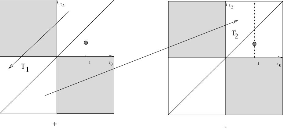
Figure 1:

Range of parameters $t_{0}$, $t_{2}$ for which the model (1) is integrable as a consequence of (1.2) for $U=+2(t_{0}-t_{2})$ (left) and $U=-2(t_{0}-t_{2})$ (right). The dots mark the model introduced in Ref. [12].

Figure 2:

Energy of the antiferromagnetic ground state of the system (1) vs. electron density in the repulsive regime for various values of the reduced coupling constant $c$. For comparison, the energy of the ferromagnetic state (4.3) is also included. Note, that for $c\to\infty$ the ferro- and antiferromagnetic states are degenerate.

Figure 3:

Energy of the antiferromagnetic ground state of the system (1) vs. electron density in the attractive regime for various values of the reduced coupling constant $c$.

Figure 4:

Energy gap for the creation of unpaired electrons as a functions of the density of particles for several values of the parameter $c$.

Figure 5:

Contours of constant $\xi_{c}(Q)$ (and hence identical critical exponents) in the $n_{e}$–$c$ parameter plane of the repulsive model. $\xi_{c}(Q)$ varies between $1$ (at low densities) and $\sqrt{2}$ (the free fermionic case) for finite $c$.

Figure 6:

Contours of constant $\xi_{p}(Q)$ (and hence identical critical exponents) in the $n_{e}$–$|c|$ parameter plane of the attractive model at small magnetic fields $h<h_{c1}$. $\xi_{p}(Q)$ varies between $1$ and $1/\sqrt{2}$ for any finite $c$.

References

- [1] E. H. Lieb and F. Y. Wu, Phys. Rev. Lett. 20, 1445 (1968).
- [2] B. Sutherland, Phys. Rev. B 12, 3795 (1975).
- [3] P. Schlottmann, Phys. Rev. B 36, 5177 (1987).
- [4] F. H. L. Eßler, V. E. Korepin, and K. Schoutens, Phys. Rev. Lett. 68, 2960 (1992).
- [5] R. Z. Bariev, A. Klümper, A. Schadschneider, and J. Zittartz, J. Phys. A 26, 1249 (1993).
- [6] J. E. Hirsch, Physica 158C, 326 (1989).
- [7] J. E. Hirsch and F. Marsiglio, Phys. Rev. B 41, 2049 (1990); F. Marsiglio and J. E. Hirsch, Phys. Rev. B 41, 6435 (1990).
- [8] J. de Boer, V. E. Korepin, and A. Schadschneider, Phys. Rev. Lett. 74, 789 (1995).
- [9] L. Arrachea and A. A. Aligia, Phys. Rev. Lett. 73, 2240 (1994).
- [10] A. J. Bracken, M. D. Gould, J. R. Links, and Y.-Z. Zhang, Phys. Rev. Lett. 74, 2768 (1995).
- [11] G. Bedürftig and H. Frahm, “Comment on ‘Model of Fermions with Correlated Hopping (Integrable Cases)”’, preprint ITP-UH-02/95.
- [12] I. N. Karnaukhov, Phys. Rev. Lett. 73, 1130 (1994).
- [13] L. D. Faddeev and L. A. Takhtajan, J. Sov. Math. 24, 241 (1984), [Zap. Nauch. Semin. LOMI 109, 134 (1981)].
- [14] C. N. Yang, Phys. Rev. Lett. 19, 1312 (1967).
- [15] C. N. Yang and C. P. Yang, J. Math. Phys. 10, 1115 (1969).
- [16] M. Takahashi, Prog. Theor. Phys. 47, 69 (1972).
- [17] C. N. Yang and C. P. Yang, Phys. Rev. 150, 327 (1966).
- [18] F. Woynarovich, J. Phys. A 22, 4243 (1989).
- [19] H. Frahm and V. E. Korepin, Phys. Rev. B 42, 10553 (1990).
- [20] N. Kawakami and S.-K. Yang, J. Phys. Condens. Matter 3, 5983 (1991).
- [21] H. Frahm and V. E. Korepin, Phys. Rev. B 43, 5653 (1991).
- [22] I. N. Karnaukhov, to be published.
- [23] N. M. Bogolyubov and V. E. Korepin, Theor. Math. Phys. 82, 231 (1990).
- [24] A. Foerster and M. Karowski, Nucl. Phys. B 396, 611 (1993).
- [25] F. H. L. Eßler, V. E. Korepin, and K. Schoutens, Nucl. Phys. B 384, 431 (1992).