[

Simple description of the anisotropic two-channel Kondo problem

Abstract

We adapt strong-coupling methods first used in the one-channel Kondo model to develop a simple description of the spin-$1\over 2$ two-channel Kondo model with channel anisotropy. Our method exploits spin-charge decoupling to develop a compactified Hamiltonian that describes the spin excitations. The structure of the fixed-point Hamiltonian and quasiparticle impurity S-matrix are incompatible with a Fermi liquid description.

]

An important question in the current debate on non-Fermi liquids concerns their stability in a real-world environment. Though it is possible to construct models with non-Fermi liquid ground-states, conventional wisdom holds that real-world perturbations absent from the model will drive a non-Fermi liquid back to a Fermi liquid. This has led to controversy in connection with two non-Fermi liquid models: the one-dimensional Luttinger liquid [1, 2], and the single impurity two-channel Kondo model, where the contentious perturbations are dimensionality [3], and channel asymmetry respectively.

In this Letter we confront this issue in the context of the asymmetric two-channel Kondo model. This model was first introduced by Nozières and Blandin [4]

$${\cal H}^{\prime}= \displaystyle it\sum_{n\lambda\sigma}[c^{\dagger}_{\lambda\sigma}(n+1)c_{\lambda\sigma}(n)-{\rm H.c}.]$$ (1)

$$\displaystyle+[J_{1}\vec{\sigma}_{1}(0)+J_{2}\vec{\sigma}_{2}(0)]\cdot\vec{S}_{d},$$ (2)

where $\lambda=1,2$ labels two independent one-dimensional conducting chains, $\vec{\sigma}_{\lambda}(0)=c^{\dagger}_{\lambda\alpha}(0)\vec{\sigma}_{\alpha\beta}c_{\lambda\beta}(0)$ is their spin density at the origin and $\vec{S}_{d}$ is a localized spin $1/2$ operator. By tuning the anisotropy $J_{2}/J_{1}$, this model interpolates continuously between a non-Fermi liquid state at the channel-isotropic point [5, 6] ($J_{2}/J_{1}=1$) and a Fermi liquid in the single channel limit [7] ($J_{2}/J_{1}=0,\infty$). Fabrizio, Gogolin and Nozières [8] have recently argued that the relevant perturbation of channel anisotropy immediately restores Fermi liquid behavior. However, when we contrast this model with the corresponding spin-$1$ model, itself a well-established Fermi liquid [4, 9], we are faced with a series of puzzling differences. A new Bethe Ansatz solution[10] shows clear qualitative differences between the excitation spectra of these two models. In particular a new type of singlet excitation present in the spin 1/2 model is absent in its spin 1 counterpart. In addition, ertain features of a two-channel Fermi liquid close to channel isotropy are expected to be universal [4]. Most notably, channel symmetry is expected to constrain the ratio of inter- and intra-channel interactions, leading to a Wilson ratio close to $8/3$. By contrast, the $S=1/2$ model exhibits vanishingly small Wilson ratios in this region,[8, 10] which require the introduction of an ad-hoc inter-chain Fermi liquid interaction of ever increasing size[8].

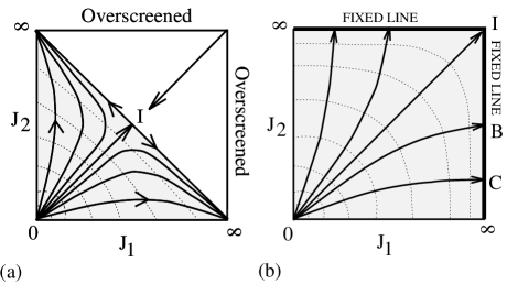
FIG. 1.: (a) Scaling trajectories for the two-channel Kondo model showing intermediate coupling fixed point and separatrix; (b) scaling trajectories of the compactified two-channel Kondo model. The beta function for the two procedures coincides at weak coupling, but in (b) the elimination of the over-screened fixed point leads to a redefinition of the coupling constants at strong-coupling that shifts the separatrix linking to infinite coupling.

We clarify these points here by using a strong-coupling expansion. A novel approach is required, because the scaling physics of the two-channel $S=1/2$ Kondo model is controlled by a separatrix at intermediate rather than infinite coupling (see Fig. 1). To overcome this difficulty, we exploit spin-charge decoupling to remove the charge degrees of freedom [11]. This procedure eliminates the over-screened fixed points, (Fig. 1) moving the attractive fixed points to infinity where a strong-coupling expansion can be made. In the fixed point Hamiltonian we derive, we find that the spin-quasiparticles occur in a $S=0$ or a triplet $S=1$ branch. Unlike the Fermi liquid description, these quasiparticles are intrinsically channel off-diagonal and their interactions are completely constrained in terms of the impurity phase shifts in such a way that the Wilson ratio drops to zero in the vicinity of channel isotropy. These results substantiate a conclusion that channel asymmetry does not restore a Fermi liquid.

The method used exploits two observations: (i) that the charge and pair degrees of freedom can be combined into a single $SU(2)$ spin operator, commonly called “isospin”,[12, 13] and (ii) that the spin and isospin variables of a single linearized conduction chain form two independent spin degrees of freedom. For a linearized one-dimensional band, the mapping

$$\begin{array}[]{rl}\vec{\sigma}_{1}(x)&\displaystyle\longleftrightarrow\vec{\sigma}(x),\\ \vec{\sigma}_{2}(x)&\displaystyle\longleftrightarrow\vec{\tau}(x),\\ \end{array}$$ (3)

where

$$\vec{\sigma_{1}} = (c^{\dagger}_{\uparrow},\ c^{\dagger}_{\downarrow})\cdot\vec{\sigma}\cdot\left(\begin{array}[]{c}c_{\uparrow}\\ c_{\downarrow}\end{array}\right)\;,$$ (6)

$$\vec{\tau} = (c^{\dagger}_{\uparrow},\;c_{\downarrow})\cdot\vec{\sigma}\cdot\left(\begin{array}[]{c}c_{\uparrow}\\ c^{\dagger}_{\downarrow}\end{array}\right)\;$$ (9)

are the spin and isospin density respectively, preserves the spin operator algebra. Under this mapping we may remove the (inert) charge degrees of freedom of the original two-channel Kondo model and compactify the spin-physics of this model into the following Hamiltonian

$${\cal H}={\cal H}_{\rm band}+{\cal H}_{\rm int}\;.$$ (10)

Here

$${\cal H}_{\rm band} = it\sum_{n}[c^{\dagger}_{\sigma}(n+1)c_{\sigma}(n)-{\rm H.c.}]\;,$$ (11)

$${\cal H}_{\rm int} = [J_{1}\vec{\sigma}(0)+J_{2}\vec{\tau}(0)]\cdot\vec{S}_{d}$$ (12)

and the spin and isospin of the single band represent respectively the spin-density of channel one and two in Eq. (2). The advantage of this procedure derives from the inability of spin and isospin to co-exist at a single site on a lattice, preventing over-screening. The unstable over-screened fixed point is thereby removed from the scaling trajectories and the scaling trajectories are deformed at strong coupling so that the (non-universal) location of the non-Fermi liquid fixed point is shifted to infinite coupling (Fig. 1).

For the conventional Kondo model, our ability to identify the ground-state as a Fermi-liquid is due to the special duality between the Anderson and Kondo models. Under this duality, the strong coupling limit of each model may be canonically transformed into the weak-coupling limit of its dual counterpart. These dual models represent two extreme limits of a single scaling trajectory. Weak coupling in the Kondo model controls the high temperature local-moment physics [14]; strong-coupling in the Kondo model controls the low-temperature physics. Duality permits us to map the strong coupling physics of the Kondo model onto an Anderson model at weak coupling with renormalized parameters [9]. This provides the basis of Nozières’ phase shift Fermi liquid description of the Kondo model [7].

We now construct the dual to the compactified two-channel Kondo model of Eq. (10). The natural language here is that of Majorana fermions, whereby the two Fermi fields are rewritten in terms of four real (Majorana) components $\Psi_{0}$ and $\vec{\Psi}$ as follows

$$\left(\begin{array}[]{c}c_{\uparrow}(n)\\ c_{\downarrow}(n)\end{array}\right)={1\over\sqrt{2}}\left(\Psi_{0}(n)+i\vec{\Psi}(n)\cdot\vec{\sigma}\right)\left(\begin{array}[]{l}0\\ -i\end{array}\right).$$ (13)

In this representation we may write

$${\cal H}_{\rm band} = it\sum_{n,\alpha=0}^{3}\Psi_{\alpha}(n+1)\Psi_{\alpha}(n)\;,$$ (14)

$${\cal H}_{\rm int} = i\left[J\vec{\Psi}(0)\times\vec{\Psi}(0)+2A\Psi_{0}(0)\vec{\Psi}(0)\right]\cdot\vec{S}_{d}\;,$$ (15)

where $J=\frac{1}{2}(J_{1}+J_{2})$ and $A=\frac{1}{2}(J_{1}-J_{2})$. Thus scalar and vector components of the conduction sea are completely decoupled in the channel symmetric model ($A=0$). By contrast, in the one-channel limit, (${A\over J}=\pm 1$) all four components of the conduction Majoranas are symmetrically coupled to the local moment, forming a model with an $O(4)\sim SU(2)\times SU(2)$ symmetry derived from spin conservation on each separate channel. The symmetric Anderson model that is dual to this limit

$${\cal H}_{A}={\cal H}_{\rm band}+iV[c^{\dagger}_{\sigma}(0)d_{\sigma}-{\rm H.c.}]+\frac{U}{2}(\hat{n}_{d}-1)^{2}\;,$$ (16)

can be rewritten in the Majorana representation to display this $O(4)$ symmetry

$${\cal H}_{A}={\cal H}_{\rm band}+iV\sum_{\alpha=0}^{3}\Psi_{\alpha}(0)d_{\alpha}-Ud_{0}d_{1}d_{2}d_{3}\;.$$ (17)

To develop the dual to the two-channel model we break the $O(4)$ symmetry in the hybridization down to an $O(3)$ symmetry, and write the following model

$${\cal H}_{M}={\cal H}_{\rm band}+i[V_{s}\Psi_{0}(0)d_{0}+V_{v}\vec{\Psi}(0)\cdot\vec{d}]-Ud_{0}d_{1}d_{2}d_{3}\;.$$ (18)

When we carry out a Schrieffer-Wolff canonical transformation that eliminates the hybridization terms, we find that the compactified two-channel model is recovered with

$$J={2(V_{v})^{2}\over U}\;,\quad\qquad A={2V_{s}V_{v}\over U}\;.$$ (19)

Once we can confirm that the compactified two-channel Kondo model scales to strong coupling, we may immediately use the Majorana resonant level model to describe the low-temperature physics.

Next, consider the stability of the large $J$ limit. For $J\gg t$, ${\cal H}_{\rm band}$ is a perturbation and the structure of the eigenstates is dominated by ${\cal H}_{\rm int}$. The eigenstates of ${\cal H}_{\rm int}$ involve two singlets and two triplets separated by an energy of order $J$. To examine the stability of this limit, we systematically develop a $t/J$ expansion. This is done by using a canonical transformation which removes, in powers of $t/J$, the mixing between the singlet and triplet subspaces. Working to order $1/J^{2}$ it is sufficient to consider only the hopping between site $0$ and site $1$ to obtain the strong coupling Hamiltonian

$$\tilde{\cal H}^{*} = \!\!it\sum_{n>0}\vec{\Psi}_{\alpha}(n+1)\cdot\vec{\Psi}(n)+it\sum_{n\geq 0}\Psi_{0}(n+1)\Psi_{0}(n)$$ (20)

$$+ iV_{s}^{*}\Psi_{0}(0)\Phi-U^{*}\Phi\Psi_{1}(1)\Psi_{2}(1)\Psi_{3}(1)\;,$$ (21)

where $U^{*}={3t^{3}/4J^{2}}$, $V_{s}^{*}=A(1-t^{2}/2J)$ and $\Phi=-2i\Psi_{1}(0)\Psi_{2}(0)\Psi_{3}(0)$ is a single Majorana field that is hybridized with the scalar fermions. By hybridizing with a zero-energy fermion, the scalar fermions experience unitary scattering, with phase-shift $\delta_{o}=\pi/2$. Since the vector fermions are excluded from the origin, they also experience unitary scattering, but with a resonance width of order $t$. The form of this Hamiltonian is thus isomorphic with ${\cal H}_{M}$ given above and since $U^{*}\ll t$, the model is weak-coupling.

The isotropic case $A=0$ has been studied in detail in previous papers [15, 16, 11]. At this point the scalar fermions decouple to form a free band of unscattered singlet excitations. The coupling $U^{*}$ between the localized Majorana $\Phi$ is a ‘dangerous irrelevant variable’. Though its vertex corrections can be neglected, it gives rise to logarithmically singular contributions to the electron self-energy and thermodynamics. At $T=0$, $\Phi$ is asymptotically decoupled from the Fermi sea, forming a fermionic zero mode. This is the feature that is responsible[15, 16] for the fractional zero-point entropy ${1\over 2}\ln 2$ [5, 6]. At finite temperatures the three-body interaction with the conduction sea can be treated perturbatively. The ‘dangerous’ terms in the free energy to lead to a logarithmic temperature dependence of the spin susceptibility $\chi_{\sigma}\sim\ln T$ and specific heat $\gamma=\frac{{\rm C}_{v}}{T}\sim\ln T$ which combine to give a dimensionless Wilson ratio of 8/3.

In the channel anisotropic case $A\neq 0$, the fermion $\Phi$ acquires a finite lifetime: $\tau_{\Phi}^{-1}=A^{2}/2t$. Processes at energies $\omega\gtrsim\tau_{\Phi}^{-1}$ are insensitive to the anisotropy. Marginal spin-physics is thus exhibited over a finite temperature range $\tau_{\Phi}^{-1}\ll T\ll t$. Once $T\ll(\tau_{\Phi}^{-1})$ the correct description will then be in terms of an effective Hamiltonian in which only the lowest lying singlet state remains. Since there is no residual degeneracy, this fixed point is stable. The scattering and interactions of the vector and scalar Majorana fermions off the singlet state will then be described by a renormalized Majorana resonant level model, of the type given above

$$\tilde{\cal H}_{M} = {\cal H}_{M}[V_{s}^{*},V_{v}^{*},U^{*}]$$ (22)

$$+ igB\left(d_{1}d_{2}-d_{0}d_{3}\right)+i\mu\left(d_{1}d_{2}+d_{0}d_{3}\right)\;,$$ (23)

where we have explicitly included a chemical potential and magnetic field in the $z$ direction.

We now use renormalized perturbation theory about $U^{*}=0$ point [9] to obtain the low-temperature thermodynamics. We work to leading order in $U^{*}$ and consider the large bandwidth limit, with a density of states $\rho$. The scalar and vector fermions develop resonant levels of width $\Delta_{s}=\pi\rho|V^{*}_{s}|^{2}$ and $\Delta_{v}=\pi\rho|V^{*}_{v}|^{2}$ respectively. The linear specific heat coefficient is then given by $\gamma_{\rm imp}=\frac{\pi^{2}}{3}\rho_{\rm imp}$, where

$$\rho_{\rm imp}={1\over 2\pi}\left({3\over\Delta_{v}}+{1\over\Delta_{s}}\right)\;.$$ (24)

FIG. 2.: Leading terms in the charge and spin susceptibilities of the impurity. Positive and negative signs are for the charge and spin susceptibility respectively.

Fig. 2 shows the diagrams that need to be calculated to determine the susceptibilities. These lead to

$$\chi_{c}^{\rm imp} = {1\over\pi\Delta_{v}}+{\ln(\Delta_{v}/\Delta_{s})\over\pi(\Delta_{v}-\Delta_{s})}\left(1-{2{U^{*}}\over\pi\Delta_{v}}\right),$$ (25)

$$\chi_{\sigma}^{\rm imp} = {1\over\pi\Delta_{v}}+{\ln(\Delta_{v}/\Delta_{s})\over\pi(\Delta_{v}-\Delta_{s})}\left(1+{2{U^{*}}\over\pi\Delta_{v}}\right).$$ (26)

Since the two-channel Kondo model corresponds to the large $U$ limit of ${\cal H}_{M}$, it follows that the renormalized calculation must lead to a vanishing charge susceptibility $\chi_{c}^{\rm imp}=0$. Using (25) to eliminate $U^{*}$, it follows that

$$\chi_{\sigma}^{\rm imp}={2\over\pi}\left[{1\over\Delta_{v}}+{\ln(\Delta_{s}/\Delta_{v})\over(\Delta_{s}-\Delta_{v})}\right]\;.$$ (27)

From (27) and (24) we obtain the Wilson ratio

$$R={\pi^{2}\over 3}{\chi_{\sigma}^{\rm imp}\over\gamma_{\rm imp}}=4\left[{1+(\ln\alpha)/(\alpha-1)\over 3+1/\alpha}\right]\;,$$ (28)

where $\alpha=\Delta_{s}/\Delta_{v}$ (see Fig. 3). This result extrapolates between $-4\alpha\ln\alpha$ at low anisotropy and $2$ as $\alpha\rightarrow 1$ (the single channel limit), in qualitative agreement with the Bethe Ansatz solution. [10] At small anisotropy, the physics is dominated by the spinless scalar fermions, and this is the origin of the small spin-susceptibility and Wilson ratio. In the thermodynamic Bethe Ansatz solution, there is a two-stage quenching of the impurity spin entropy: below $T_{K}$ the entropy saturates at ${1\over 2}\ln 2$ before quenching to $0$ at a new low energy scale. We may identify this second scale with $\tau_{\Phi}^{-1}$. In the isotropic limit, the Wilson ratio found by Bethe Ansatz goes vanishes as $R\sim-\Delta\ln\Delta$ (where $\Delta$ is the ratio of the two energy scales) in exactly the same fashion as the calculation presented above.

FIG. 3.: The dimensionless Wilson ratio, $\chi^{\rm imp}_{\sigma}/\gamma_{\rm imp}$, as a function of the anisotropy $\alpha=\Delta_{s}/\Delta_{v}$ [see Eq. (28)].

We now turn to the question of whether this state is a Fermi liquid. Using Eq. (3) we identify the total spin of the excitations as $\vec{S}=(\vec{\sigma}+\vec{\tau})/2$. At the fixed point, the spin-excitations in the two channels combine into two types of spin excitation, a singlet and a triplet represented by the scalar and vector Majorana fermions:

$$S = 0\quad\quad\Psi^{\dagger}_{0}(k)|0\rangle\;,$$ (29)

$$S = 1\quad\left\{\begin{array}[]{lc}S_{z}=\pm 1&{1\over\sqrt{2}}[\Psi^{\dagger}_{1}(k)\pm i\Psi^{\dagger}_{2}(k)]|0\rangle\\ S_{z}=0&\Psi^{\dagger}_{3}(k)|0\rangle\end{array}\right.\;,$$ (32)

where $0<k<\pi$. These excitations are formed by correlating the spins across the two channels—a feature reminiscent of the ‘spin fusion’ process that plays a central rôle in the Bethe Ansatz solution[5, 10]. At the isotropic point, the scalar excitations decouple from the impurity. This is confirmed by the Bethe Ansatz solution, which shows that the linear specific heat capacity of the conduction sea increases by a factor of $4/3$ in going from the isotropic to the anisotropic solutions[17]. From the fixed point Hamiltonian, we deduce that the one-particle S-matrix of the spin excitations has the form

$$S_{\rm 2-channel}=e^{2i\delta_{s}(\epsilon)}{\cal P}_{s}+e^{2i\delta_{v}(\epsilon)}{\cal P}_{v}\;,$$ (33)

where $\delta_{s,v}(\epsilon)={\pi\over 2}+{\rm tan^{-1}}\left(\displaystyle\epsilon\over\Delta_{s,v}\right)\;$ and

$${\cal P}_{v}=\frac{1}{4}\left[3+\vec{\sigma}\cdot\vec{\tau})\right]\;\;,\;\;{\cal P}_{s}=\frac{1}{4}\left[1-\vec{\sigma}\cdot\vec{\tau})\right]\;,$$ (34)

project the excitations into the singlet and triplet channel [18]. This S-matrix is explicitly channel off-diagonal. Were the ground-state a Fermi liquid, the one-quasiparticle S-matrix would be channel diagonal, with spin-${1\over 2}$ quasiparticles that are individually confined to a definite channel. Unlike the Fermi liquid description, the quasiparticle interaction is completely constrained by the phase shifts, and does not need to be adjusted to fit results obtained by other methods.

These fundamental discrepancies between the spin excitation spectrum of the anisotropic $S={1\over 2}$ two-channel Kondo model and those of a two channel Fermi liquid indicate that spin-charge decoupling is an essential feature of two-channel Kondo physics; they enable us to understand why the spin-$1$ and spin-${1\over 2}$ models are so different in the vicinity of the isotropic point. We have seen how the triplet and singlet spin excitations take advantage of spin-charge decoupling to form quasiparticles that are delocalized between channels in a fashion that does not occur for rigidly defined electron quasiparticles. In this respect, the anisotropic two-channel spin-$1\over 2$ Kondo model is reminiscent of the Luttinger liquid: although it displays similar thermodynamics to a Fermi liquid, its spin-charge decoupled excitations can not be recast in Fermi liquid form.This result is of potential practical importance in systems governed by single-impurity two-channel Kondo physics, for it ensures the survival of non-Fermi liquid behavior even when channel asymmetry is destroyed. Equally important, our results refute the conventional wisdom, demonstrating that a relevant perturbation to a non-Fermi liquid state does not inevitably restore an electron Fermi liquid.

We acknowledge many informative discussions with N. Andrei, A. Jerez and A. Tsvelik and would like to thank Ph. Nozières for his comments on an early version of this work. This work was supported by NSF grant DMR-93-12138. A.J.S. is supported by a Royal Society NATO post-doctoral fellowship.

REFERENCES

- [1] F. D. M. Haldane, J. Phys. C 14, 2585 (1981) and references therein.
- [2] P. W. Anderson, Phys. Rev. Lett. 64, 1839 (1990).
- [3] A. M. Finkel’stein and A. I. Larkin, Phys. Rev. B 47, 10461 (1993); M. Fabrizio and A. Parola, Phys. Rev. Lett. 70, 226 (1993).
- [4] Ph. Nozières and A. Blandin, J. Phys. (Paris) 41, 193 (1980).
- [5] N. Andrei and C. Destri, Phys. Rev. Lett. 52, 364 (1984).
- [6] A. M. Tsvelik and P. B. Wiegmann, Z. Phys. B 54, 201 (1984).
- [7] Ph. Nozières, J. Low Temp. Phys. 17, 31 (1974).
- [8] M. Fabrizio, A. Gogolin and Ph. Nozières, Phys. Rev. Lett. 74, 4503 (1995).
- [9] A. C. Hewson, Phys. Rev. Lett. 70, 4007 (1993).
- [10] N. Andrei and A. Jerez, Phys. Rev. Lett. 74, 4507 (1995).
- [11] P. Coleman, L. B. Ioffe and A. M. Tsvelik, to be published.
- [12] P. W. Anderson, Phys. Rev. 112, 1900, (1958).
- [13] Y. Nambu, Phys. Rev. 117, 648, (1960).
- [14] J. R. Schrieffer and P. A. Wolff, Phys. Rev. 149, 491 (1966).
- [15] V. J. Emery and S. Kivelson, Phys. Rev. B 46, 10812 (1992).
- [16] A. M. Sengupta and A. Georges, Phys. Rev. B 49, 10020 (1994).
- [17] We are grateful to A. Tsvelik for pointing this out.
- [18] can be written explicitly using a Balian Werthamer four-component notation for the conduction electron fields, where and are the spin and isospin operators in this basis. See e.g. R. Balian and N. R. Werthamer, Phys. Rev. 131, 1553 (1963).