[

NSF–ITP–95–35, cond-mat/9504082
Temporal Order in Dirty Driven Periodic Media

Abstract

We consider the non–equilibrium steady states of a driven charge density wave in the presence of impurities and noise. In three dimensions at strong drive, a true dynamical phase transition into a temporally periodic state with quasi–long–range translational order is predicted. In two dimensions, impurity induced phase slips are argued to destroy the periodic “moving solid” phase. Implications for narrow band noise measurements and relevance to other driven periodic media, e.g. vortex lattices, are discussed.

]

The influence of quenched impurities on a periodic medium can lead to very rich physics. Examples include charge density wave (CDW) systems[1] and the mixed state of type II superconductors[2], in which the vortices form a periodic lattice. In both these cases, it has been argued that the impurities ultimately destroy the long-ranged periodicity and pin the periodic medium. However, with an applied force, provided by an electric field or current, the periodic structure de-pins and becomes mobile. Once in motion, the impurities are less effective at destroying the periodicity. Indeed, recent experiments on YBaCuO have shown evidence for a first order melting transition of the moving vortex lattice[3]. Vinokur and Koshelev have interpreted this experiment in terms of a true non-equilibrium phase transition, from a moving liquid phase to a “moving solid phase”[4].

This experiment raises a number of questions about the non-equilibrium steady states of such noisy driven systems with impurities. The most basic concerns the very existence of a “moving solid” phase. A solid in equilibrium is usually characterized by the presence of long-ranged crystalline correlations (Bragg peaks). But other criteria also suffice, such as the presence of a non-zero shear modulus, or the absence of unbound dislocation loops. Under what circumstances, if any, is it possible to have a true moving solid, separate from a driven liquid with plastic flow? If the moving solid phase is possible, what are it’s characteristics and experimental signatures?

In this letter we attempt to answer these questions, focusing for simplicity on the CDW. Many of our conclusions, however, apply also to the driven vortex lattice. In two dimensions, we find that a moving solid phase driven through impurities is always unstable to a proliferation of dislocations. The system becomes equivalent (in symmetry) to a driven liquid. In three dimensions, a moving solid phase appears to be stable at large velocities, as illustrated in the schematic phase diagram, Fig.1. However, the solid phase does not have true long-ranged positional correlations (LRO), as in an equilibrium (3d) crystal. Rather, algebraic power law positional correlations are predicted, as in a 2d equilibrium crystal. Likewise, unbound dislocation loops are absent in the moving solid. Despite the absence of spatial LRO, the moving solid phase is periodic in time – and hence has long-ranged temporal correlations. The experimental signature of such a periodic state is narrow band noise, at the “washboard” frequency[1, 5].

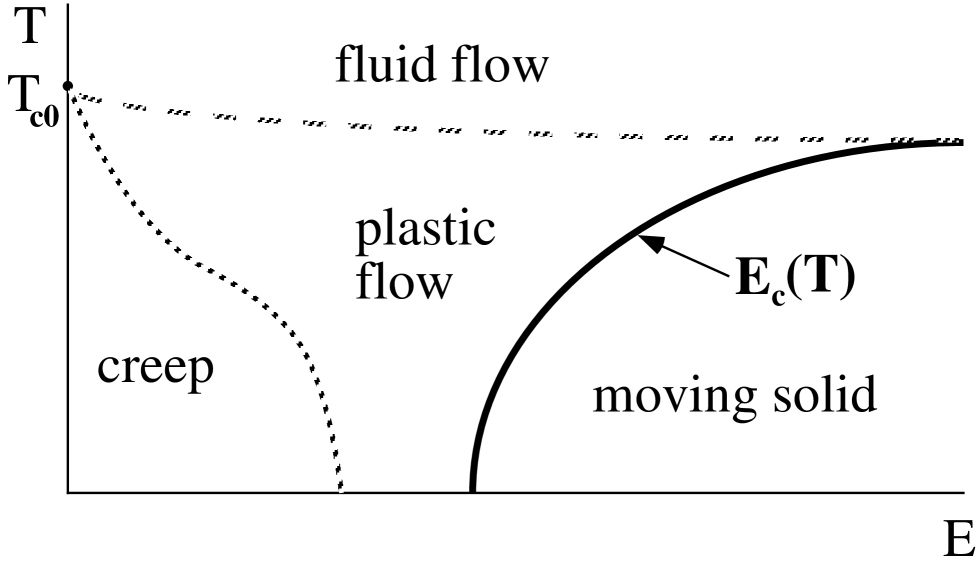
FIG. 1.: Schematic phase diagram for the three-dimensional CDW. Hashed lines indicate (possibly sharp) crossovers.

Upon inclusion of thermal effects or phase slips, the CDW de-pinning transition[6] is predicted to be rounded[7], becoming a crossover (see Fig.1). For electric fields, $E$, above this crossover, the CDW is in a plastic flow regime. With increasing $E$, we predict a true phase transition into a temporally periodic “moving solid” phase. For the CDW, this dynamical transition is likely to be continuous. As shown below, scaling arguments then predict NBN characteristics near the transition. The phase diagram for the driven vortex lattice should be similar, with current replacing electric field. However, in this case the transition into the moving solid phase is likely to be first order, at least in the large current limit.

Charge density waves tend to form in very anisotropic metals, consisting of weakly coupled metallic chains[1]. The electronic density in a CDW has a periodic modulation along the chain (x-)direction:

$$\rho({\bf x})=\rho_{0}+{\rm Re}\psi e^{i2k_{\rm F}x},$$ (1)

with $k_{\rm F}$ the in-chain Fermi wave vector. Long-ranged order of the CDW is manifest in the complex order parameter field, $\psi({\bf x})=\rho_{1}e^{i\phi}$.

In the absence of impurities and an applied electric field, the CDW exhibits long-ranged order in the pair correlation function:

$$G({\bf x})=<\psi^{*}({\bf x},t)\psi({\bf 0},t)>_{t},$$ (2)

with $G(x\rightarrow\infty)\neq 0$. Here the subscript $t$ denotes a time average (equivalently an ensemble average in equilibrium). Lee and Rice have argued that quenched impurities destroy the LRO of $G$, for physical dimensions, $d<4$[8]. However, when the CDW is driven and moving, the Lee-Rice argument is not valid, and LRO of $G$ is not precluded (but see below).

In the moving non-equilibrium steady state, temporal correlations in $\psi$ also serve to characterize the CDW order. Consider the pair correlation function:

$$C(t)=<\psi^{*}({\bf x},t)\psi({\bf x},0)>_{x},$$ (3)

where the subscript $x$ denotes a spatial average. Temporal LRO is signaled by a periodic, and non-decaying, behavior: $C(t+t_{0})=C(t)$, with $t_{0}$ the “washboard’ period. Middleton has shown that for a large class of dynamical models, which exclude phase slip and thermal noise, the steady state is (microscopically) periodic[9]. With noise microscopic periodicity is destroyed, but the statistical correlation function $C(t)$ is still periodic. However, when phase slip is allowed, the robustness of the periodic state is much less clear, as we discuss below.

To proceed, we assume local CDW order, and construct a long wavelength description in terms of $\psi$. In the absence of phase slips, as we consider first, amplitude fluctuations can be ignored, and the dynamics involves the phase field, $\phi$. A common starting point is the Fukuyama-Lee-Rice (FLR) model[10], with equation of motion:

$$\partial_{t}\phi=D\nabla^{2}\phi+V({\bf x})\sin(2k_{\rm F}x+\phi)+v2k_{\rm F}.$$ (4)

The spatial coordinates transverse to the chains have been re-scaled to give an isotropic diffusion constant $D=\tau v_{\rm F}^{2}$, with scattering time $\tau$ and Fermi velocity $v_{\rm F}$. The second term on the right side represents the effect of quenched random impurities. The last term is present in an applied electric field $E$, with velocity $v=(e\tau/m)E$. This term can be shifted away, $\phi\rightarrow\phi+v2k_{\rm F}t$, reducing the FLR equation to an equilibrium form: $\partial_{t}\phi=-\delta H/\delta\phi$, with Hamiltonian $H$. However, there are additional terms that can, and should, be added to FLR, which are manifestly non-equilibrium, as we now discuss.

The most important such term is $\partial_{x}\phi$, allowed by symmetry once the CDW is in motion along the $x$-direction. The magnitude of this term can be estimated by balancing forces on a single wavelength, $\lambda$, of one chain. In an electric field E, the force is $2eE$, accelerating (locally) the phase field: $2m\partial_{t}^{2}(\lambda\phi/2\pi)=2eE$, or equivalently, $\tau\partial_{t}^{2}\phi=v2\pi/\lambda$. In the presence of distortions in $\phi(x)$, the (local) wavelength of the CDW is modified: $2\pi/\lambda\rightarrow 2k_{\rm F}+\partial_{x}\phi$. Thus the last term in FLR should be replaced by: $2k_{\rm F}\rightarrow 2k_{\rm F}+\partial_{x}\phi$. (Note that the inertial term has been dropped.)

In general there are other missing terms, for example of the KPZ form, $(\partial_{x}\phi)^{2}$[11]. This term, involving more gradients and powers of $\phi$ is less relevant than $\partial_{x}\phi$. In the following we drop this term, although it can play an important role[12].

In the moving state, it is tempting to argue that the impurity term, $V(x)$, will average to zero at long times. However, as pointed out by Coppersmith[7], it is not legitimate to ignore completely the effect of impurities. In particular, the impurities modify the local mobility, $\mu$, of the phase field. (This can be seen explicitly via a high velocity expansion.) The random $V$ term can then be replaced by $\delta\mu(x)E2k_{\rm F}=F(x)$, where $\delta\mu$ denotes the fluctuating part of the mobility. We take $F$ Gaussian with $\overline{F}=0$ and $\overline{F({\bf x})F({\bf 0})}=g\delta({\bf x})$.

We thereby arrive at a generalization of FLR:

$$\partial_{t}\phi=D\nabla^{2}\phi+v(2k_{\rm F}+\partial_{x}\phi)+F({\bf x})+\eta({\bf x},t).$$ (5)

The stochastic noise term is assumed to be Gaussian with $\langle\eta\rangle=0$ and $\langle\eta({\bf x},t)\eta({\bf x}^{\prime},t^{\prime})\rangle=k_{B}T\delta({\bf x-x^{\prime}})\delta(t-t^{\prime})$.

Finally, we modify the model to allow for phase slip processes. One way to incorporate phase slip is to put the model on a lattice and replace $\partial_{x}\phi\rightarrow a^{-1}sin(\phi(x+a)-\phi(x))$, etc. Alternatively, amplitude fluctuations can be included, using field $\psi$. The appropriate soft-spin model, which reduces to Eq.5 in the spin-wave limit, is,

$$\partial_{t}\psi = [D\nabla^{2}+v\partial_{x}+M+r({\bf x})+i\omega_{0}+iF({\bf x})]\psi$$ (7)

$$-u\psi|\psi|^{2}+\xi({\bf x},t),$$

with the definition $\omega_{0}=v2k_{\rm F}$. Here $M$ is a “mass” term, which controls the magnitude of the order parameter, and $\xi({\bf x},t)$ is a complex stochastic noise term. We have also included a spatially random component to the mass, denoted $r({\bf x})$, which we take to be a zero–mean Gaussian random variable with $\overline{r({\bf x})r({\bf 0})}=\Delta\delta({\bf x})$.

First consider the system with phase slips suppressed. In this spin–wave limit, Eq.5 is linear in $\phi$ and can be solved via Fourier transforms:

$$\tilde{\phi}({\bf p},\omega)={{F({\bf p})}\over{Dp^{2}+ivp_{x}}}2\pi\delta(\omega)+{{\eta({\bf p},\omega)}\over{i\omega+Dp^{2}+ivp_{x}}},$$ (8)

where $\tilde{\phi}(t)=\phi(t)-\omega_{0}t$. The first term in Eq.8 represents a static distortion in $\phi(x)$ induced by the random mobility, while the second gives “noisy” dynamical fluctuations around this mean. The static phase variations diverge algebraically with system size $L$ for $d<3$, leading to (stretched) exponential decay of $G(x)$. Thus, even without phase slips, a 2d driven CDW lacks translational LRO. For the 3d case, Eq.8 gives $G_{\rm sw}(x)\sim x^{-\eta}$, corresponding to power law peaks in the static structure function and translational quasi–LRO (QLRO). Notice that the presence of the non-zero $v\partial_{x}\phi$ term in Eq.5 is critical here. Indeed, for a driven periodic system with reflection symmetry, $v=0$, Eq.8 implies exponential decay of $G(x)$ for all $d<4$. Because the disorder term in Eq.8 is static, the dynamical properties are determined by the thermal noise term, with $C_{sw}(\omega)\sim\delta(\omega-\omega_{0})$ for all $d>2$, indicating temporal LRO of $C(t)$. In 2d spin-waves imply temporal QLRO for $C(t)$.

We now address the stability of these spin-wave results in the presence of phase slips. In equilibrium, $v=F=0$, Eq.7 describes an XY model with relaxational dynamics. In this case the unbinding of topological defects (i.e.. vortices) coincides with the loss of translational LRO due to spin wave fluctuations. For $d>2$, the vortices form $d-2$ dimensional subspaces (lines in 3d). With a core energy growing with size $L$ as $L^{d-2}$, they are bound at low temperatures. In equilibrium, 2d is marginal both for spin waves, which give QLRO, and for vortex unbinding. But in the non-equilibrium case of interest, the unbinding of phase slips and vortices needs to be re-addressed.

For simplicity, consider first the case $v=0$. Then Eq.5 can actually be cast into an equilibrium form, $\partial_{t}\phi=-\delta E_{\rm eff}/\delta\phi+\eta$, with the proviso that the “energy” $E_{\rm eff}=\int\{D|\nabla\phi|^{2}/2-F\phi\}$ is a multi–valued (i.e. non–periodic) function of the phase. The situation is analogous to the “tilted washboard” model of Josephson junctions, except that the tilt is here a random function of position.

It is clear that spin–wave conformations of the phase are highly constrained. Imagine sub–dividing the system into regions of linear size $L$. Each such region experiences a net random torque $\int d^{d}{\bf r}F({\bf r})$ of order $\pm\sqrt{gL^{d}}$. The torque in neighboring regions is generally different, so that the local phases are pushed at different rates. In the absence of phase slips, however, all regions must rotate synchronously or build up enormous strains. Eq.8 describes the resulting steady state in which the strains increase to counteract the non–uniform applied torques.

Once phase slips are allowed, however, such a situation is clearly metastable. If the net torque in a particular region is positive, then the energy of the spin–wave state is lowered simply by increasing all the phases in the region $L$ by $2\pi$. This decreases the random energy but does not alter the strain energy (which is now periodic in $\phi$). For finite $L$ and non–zero $T$, this process will therefore occur with an activated rate $1/\tau\sim\exp(-U/k_{\rm B}T)$, where $U$ is the energy barrier for the phase slip process.

The energy $U$ is estimated from the elastic energy mid–way through the process, i.e. when there exist phase shifts of order $\pi$ on scale $L$. Adding the elastic and random contributions to the energy gives $U(L)\sim DL^{d-2}-\sqrt{gL^{d}}$. A more microscopic picture is that of vortex nucleation. The phase slip is achieved by nucleating a small neutral topological defect (vortex–antivortex pair or vortex loop in $d=2,3$), which expands and slips over the region, annihilating again on the opposite side. The elastic contribution to the barrier energy is just the binding potential of the defect, $V_{\rm defect}(L)\sim DL^{d-2}$, up to possible $\ln L$ dependence. For $d>4$ and small $g$, $U(L)$ is positive. Moreover, since $U(L)$ grows with large $L$ large phase slips are exponentially suppressed, indicating stability of the spin-wave phase for $d>4$. For $d<4$, however, $U(L)$ becomes negative for $L>L_{c}\sim(D^{2}/g)^{1/(4-d)}$. On scales much bigger than $L_{c}$ it is then inconsistent to assume a well defined average phase, because of the proliferation of vortex pairs/loops on smaller scales. The relaxation time for the phase slips on scale $L_{c}$ is $\tau_{c}\sim\exp[DL_{c}^{d-2}/k_{\rm B}T]$. Beyond this time scale, phases separated by distance large compared to $L_{c}$ will become de-phased, destroying the temporal LRO of the spin-wave state.

For $v\neq 0$, the argument is trickier. First, transform to the moving frame via $x\rightarrow x-vt$, which removes the $v\partial_{x}\phi$ term in Eq.5. The elastic force is invariant under such a transformation, but $F({\bf r})\rightarrow F(x-vt,{\bf r}_{\perp})$, so that the random torque field appears to move with velocity $v$. Again dividing the system into regions of size $L$, we see that a statistically uncorrelated realization of $F$ moves into a particular region in a time $t_{0}=L/v$. For large $L$ this decorrelation time $t_{0}$ is much smaller than the typical diffusive time for phase changes, $t_{\phi}\sim L^{2}/D$. Only on time scales longer than $t_{\phi}$ can a phase change take advantage of the random torques spread out over the entire region. The random energy gained is thus averaged over $t_{\phi}/t_{0}$ realizations of the torques, leading to a net torque on the entire region of $F_{\rm net}\sim\sqrt{g/v}L^{(d-1)/2}$. In this case the characteristic energy balance is $U(L)\sim DL^{d-2}-\sqrt{g/v}L^{(d-1)/2}$, and phase slips proliferate for $d>3$. Directly in $d=3$, these naive arguments suggest a transition between an ordered state for $v>v_{c}$ and a disordered state for $v<v_{c}$, with $v_{c}\sim g/D^{2}$.

The above arguments are consistent with the spin–wave calculations. As in equilibrium, they suggest that vortex unbinding coincides with the loss of translational LRO due to spin-wave variations. Further support for this conclusion follows from an analysis of the soft spin model, Eq.7, as we now describe.

In the absence of randomness, the soft spin model contains two phases for $d\geq 2$. Fluctuation effects near the transition, negligible above $d=4$, can be studied for small $\epsilon=4-d$ via the renormalization group (RG). The RG including $r({\bf x})$ has been studied in the context of random–bond XY magnets[13]; we generalize this calculation to include $F$ in the dynamics (for $v=0$). After transforming $\psi\rightarrow e^{i\omega_{0}t}\psi$, we employ standard dynamical RG methods. The resulting differential RG flow equations to quadratic order are,

$$\dot{u} = u(\epsilon-5u+6\Delta),$$ (9)

$$\dot{\Delta} = \Delta(\epsilon-4u+4\Delta-2g)+2g^{2},$$ (10)

$$\dot{g} = g(\epsilon-2g+6\Delta),$$ (11)

with $\dot{u}=du/d\ln b$, etc., where $b=e^{\ell}$ is the rescaling factor. A simple analysis shows that the Gaussian ($u=\Delta=g=0$), pure ($\Delta=g=0$) and dirty equilibrium ($g=0$) fixed points are all unstable, and further, that no other fixed points exist. Instead the couplings diverge as $\ell\rightarrow\infty$. In particular, $u\rightarrow+\infty$ (not $-\infty$), so the instability does not appear to indicate a fluctuation induced first order transition. Instead, the strong divergence of the disorder strengths $g$ and $\Delta$ are consistent with the scenario that the ordered phase is absent.

For $v\neq 0$, changing to co–moving coordinates $x\rightarrow x-vt$ reduces Eq.7 to the previous case but with $r({\bf x})\rightarrow r(x-vt,{\bf x}_{\perp})$ and $F({\bf x})\rightarrow F(x-vt,{\bf x}_{\perp})$. Because $z=2+O(\epsilon)$ at the pure XY fixed point, the weaker $x$ dependence of $r$ and $F$ may be ignored. Perturbations of the form $r(-vt,{\bf x}_{\perp})\psi$ and $iF(-vt,{\bf x}_{\perp})\psi$ are strongly irrelevant near $d=4$, consistent with the spin-wave analysis and our earlier scaling arguments which gave d=3 as the lower critical dimension for the ordered phase. To study d=3 in the soft spin representation, we employ non-perturbative techniques. We therefore consider a generalized model containing $N$ complex fields $\psi_{i}$ obeying Eq.7, but with $|\psi|^{2}\rightarrow\sum_{i}|\psi_{i}|^{2}$. We analyze the stability of the pure $N=\infty$ fixed point to the random perturbations. From scaling the singular part of the mean energy density varies as $\overline{\langle\psi^{2}\rangle}=\xi^{1/\nu-d}f(\Delta\xi^{y_{\Delta}},g\xi^{y_{g}})$, where $\xi\sim M^{-1/\nu}$ is the (pure) correlation length, and $y_{\Delta}$ and $y_{g}$ are the RG eigenvalues of $\Delta$ and $g$, respectively. At $N=\infty$, $1/\nu-d=-2$. Differentiation implies $A_{\Delta}\equiv\partial_{\Delta}\overline{\langle\psi^{2}\rangle}|_{\Delta,g=0}\sim\xi^{y_{\Delta}-2}$, $A_{g}\equiv\partial_{g}\overline{\langle\psi^{2}\rangle}|_{\Delta,g=0}\sim\xi^{y_{g}-2}$. These quantities are computed at $N=\infty$ using saddle point techniques and the Martin–Siggia–Rose dynamical formalism[14]. We find $y_{\Delta}=d-5$ and $y_{g}=3-d$. (As a check we also considered the case $v=0$, and found $y_{\Delta}=d-4$ and $y_{g}=4-d$, in agreement with the usual Harris criterion and the $\epsilon$-expansion, Eq.11.) Thus for $d<3$, the equilibrium critical point is unstable to random $F$, consistent with the absence of an ordered phase.

Our predictions for the 3d phase diagram are summarized in Fig.1. Upon lowering the temperature at weak drive, $E$, substantial CDW amplitude develops at the mean-field transition temperature $T_{c0}$. At long distances and times, however, both $G(x)$ and $C(t)$ decay exponentially to zero. With increasing drive, the CDW undergoes a sharp non-equilibrium phase transition into an ordered “periodic state” with spatial QLRO and temporal LRO. Our arguments strongly suggest that for 2d CDW systems, the ordered phase is absent.

Experimentally, temporal LRO in the solid phase manifests itself in NBN. Consider current fluctuations in the presence of a fixed bias voltage; other set–ups are qualitatively similar. The current density $j({\bf x})=(en_{\perp}/\pi)\partial_{t}\phi[1+(\rho_{1}/2k_{\rm F})\cos(2k_{\rm F}x+\phi)]$, where $n_{\perp}$ is the areal chain density. In a sample of cross–sectional area $A$, the instantaneous CDW current through the plane $x=0$ is $I_{\times}(t)=\int_{A}\!d^{2}{\bf x}_{\perp}j(x=0,{\bf x}_{\perp},t)$. The oscillatory part of the NBN correlator, $S(t)\equiv\langle I_{\times}(t)I_{\times}(0)\rangle$ is thus

$$S_{o}(t)\approx I_{0}^{2}\int_{\bf x_{\perp},x_{\perp}^{\prime}}\!\!\!\!\!\!{\rm Re}\{e^{i\omega_{0}t}\left\langle\psi({\bf x_{\perp}},t)\psi^{*}({\bf x_{\perp}^{\prime}},0)\right\rangle\},$$ (12)

where $I_{0}=(en_{\perp}\omega_{0})/(2\sqrt{2}k_{\rm F}\pi)$. We consider this quantity in the bulk, and expect that measured current fluctuations (in the external leads) exhibit proportional behavior. Temporal LRO in the solid phase therefore implies a sharp (resolution limited) delta function peak in $S(\omega)\sim A^{2-\eta/2}\delta(\omega-\omega_{0})$. Deep in the liquid phase, $\psi$ correlations are short–range in space and time, which gives the mean–field result $S(\omega)\sim A\Omega/(\Omega^{2}+(\omega-\omega_{0})^{2})$. Near the transition field $E_{c}(T)$, provided the transition is continuous, we expect a scaling form $S_{\pm}(\omega,\delta E)\sim|\delta E|^{a}f_{\pm}[(\omega-\omega_{0})/|\delta E|^{z\nu},A|\delta E|^{2\nu}]$, where $z$ and $\nu$ are the dynamical and correlation length exponents, $a$ is an additional scaling exponent, and $\delta E=E-E_{c}$. Matching to the infinite area limit implies that the amplitude of the delta function frequency peak for $E>E_{c}$ vanishes as $|\delta E|^{a+(4+z-\eta)\nu}$. For $E<E_{c}$, matching implies the (generally non–Lorentzian) line-shape $S(\omega)\sim A|\delta E|^{a+2\nu}s[(\omega-\omega_{0})/|\delta E|^{z\nu}]$. In two dimensions, $S(\omega)$ has an intrinsic width for all fields and temperatures.

Although the discussion has focused on CDWs, most of the ideas employed here apply to more general periodic media. Of particular current experimental interest are vortex lattices and 2d Wigner crystals[15]. In all cases, translational and temporal LRO may be destabilized both by phonons (phase fluctuations) and by topological defects (phase slips). Provided reflection invariance is broken by an external drive field, we expect linear gradient terms (e.g. $v\partial_{x}\phi$) in the equations of motion. Preliminary investigation of driven lattices suggests that such terms play a similar role in that case[12]. There are also examples of oscillatory states in pattern forming systems without broken reflection symmetry – leading, we expect, to the absence of the ordered phase in the presence of disorder and noise.

We are grateful to J. Krug, D.S. Fisher, and G. Grinstein for helpful conversations. This work has been supported by the National Science Foundation under grants No. PHY94–07194 and No. DMR–9400142.

REFERENCES

- [1] G. Grüner, Rev. Mod. Phys. 60, 1129 (1988).
- [2] D. S. Fisher, M. P. A. Fisher, and D. A. Huse, Phys. Rev. B 43, 130 (1991); and references therein.
- [3] H. Safar et. al., unpublished. See also, A. C. Marley, M. J. Higgins, and S. Bhattacharya, Phys. Rev. Lett. 74, 3029 (1995).
- [4] A. E. Koshelev and V. M. Vinokur, Phys. Rev. Lett. 73, 3580 (1994).
- [5] J. M. Harris, N. P. Ong, R. Gagnon, and L. Taillefer, unpublished.
- [6] O. Narayan and D. S. Fisher, Phys. Rev. B 46, 11520 (1992); and references therein.
- [7] S. N. Coppersmith and A. J. Millis, Phys. Rev. B 44, 7799 (1991).
- [8] P. A. Lee and T. M. Rice, Phys. Rev. B 19, 3970, (1979).
- [9] A. A. Middleton, Phys. Rev. Lett. 68, 670 (1992).
- [10] H. Fukuyama and P. A. Lee, Phys. Rev. B 17, 535 (1978).
- [11] J. Krug, unpublished; M. Kardar, G. Parisi, and Y.-C. Zhang, Phys. Rev. Lett. 56, 889 (1986).
- [12] L.–W. Chen, L. Balents, M. P. A. Fisher, and M. C. Marchetti, unpublished.
- [13] G. Grinstein, S. Ma and G. Mazenko, Phys. Rev. B 15, 258 (1977). T. C. Lubensky, Phys. Rev. B 11, 3573 (1975).
- [14] P. C. Martin, E. D. Siggia and H.A. Rose, Phys. Rev. B 8, 423 (1973).
- [15] Y. P. Li et. al., Phys. Rev. Lett. 67, 1630 (1991); and references therein.