Critical point and coexistence curve properties of the Lennard-Jones fluid: A finite-size scaling study.

Abstract

Monte Carlo simulations within the grand canonical ensemble are used to explore the liquid-vapour coexistence curve and critical point properties of the Lennard-Jones fluid. Attention is focused on the joint distribution of density and energy fluctuations at coexistence. In the vicinity of the critical point, this distribution is analysed using mixed-field finite-size scaling techniques aided by histogram reweighting methods. The analysis yields highly accurate estimates of the critical point parameters, as well as exposing the size and character of corrections to scaling. In the sub-critical coexistence region the density distribution is obtained by combining multicanonical simulations with histogram reweighting techniques. It is demonstrated that this procedure permits an efficient and accurate mapping of the coexistence curve, even deep within the two phase region.

I Introduction

The Lennard-Jones (LJ) fluid constitutes the prototype model for realistic atomic fluids and has been the focus of numerous simulation studies spanning well over 25 years [1, 2, 3, 4, 5, 6, 7, 8, 9, 10, 11]. The motivation for the longstanding interest in the model is its utility as a test-bed for ever more accurate and sophisticated theories of the liquid state. Contemporary theories [13, 14, 15] now provide good agreement with simulation results over a wide range of noncritical temperatures. The continuing challenge, however, is to realise a similar degree of accuracy in the critical region, where the unbounded growth of correlations poses potentially serious difficulties for theory and simulation alike.

One popular simulation method for studying the coexistence regime of fluid systems is the Gibbs ensemble Monte Carlo simulation technique (GEMC) introduced by Panagiotopoulos [7]. In the GEMC method, the two coexisting phases separate into two physically detached, but thermodynamically connected boxes, the volumes of which are allowed to fluctuate under a constant pressure environment. Measurements of the particle density in each box provide estimates of the coexistence densities. Common practice is to fit the temperature dependence of these densities using a power law, the extrapolation of which yields estimates of the critical point parameters. The strength of the GEMC method lies in its elimination of the physical interface between the coexistence phases, the large free energy of which, plagues conventional grand canonical simulations of phase coexistence in the form of long lived metastable states and extended tunneling times. A large number of recent GEMC studies [16] testify to the method’s efficacy in determining the subcritical coexistence properties of fluids.

In the neighbourhood of the critical point, however, and for reasons discussed in references [17, 18, 19, 20], the GEMC method cannot be relied upon to provide accurate estimates of the coexistence curve parameters. Instead it is necessary to employ finite-size scaling (FSS) techniques to probe the critical limit. FSS techniques were originally developed in the context of computer simulation studies of critical phenomena in spin models, and provide a highly effective route to infinite volume critical parameters from simulations of finite size [21, 22]. Recently their use has been extended to fluids by explicitly incorporating the consequences of the lack of symmetry between the coexisting phases [17, 23, 24, 25]. This reduced symmetry of fluids with respect to magnetic systems such as the Ising model, is manifest in the so-called ‘field-mixing’ phenomenon which is a crucial issue in the critical behaviour of fluids. The mixed-field FSS theory has been successfully employed in conjunction with simulations in the grand canonical ensemble (GCE) to study the critical behaviour of a number of critical fluid systems [17, 23, 24, 25, 26], including the two dimensional LJ fluid and a three dimensional lattice model for polymer mixtures. In the present work we extend these studies to the 3D LJ fluid making additional use of two important new methodological advances in computer simulation.

The essential ideas underpinning the FSS methods we shall use, are the dual concepts of scale invariance and universality. Precisely at criticality, the fluctuation spectra (distribution functions) of certain readily accessible observables assume scale invariant forms [27, 28, 29]. Moreover these critical scaling functions are universal, being identical for all members of the same universality class. Experimental [30, 31, 32], theoretical [33, 34] and simulation [23] results show that the critical behaviour of simple fluids corresponds to the Ising universality class (to which all systems with short range interactions and a scalar order parameter belong). Scaling functions measured for the critical Ising model therefore constitute a hallmark of the Ising universality class, a fact that can be exploited to obtain accurate estimates of the critical point parameters of simple fluids.

Besides the progress in extending the application of FSS concepts to fluid systems, two recent technical advances in computer simulation methods also greatly improve the efficiency with which one can tackle both the critical and subcritical regimes of model systems. The first is the histogram reweighting technique of Ferrenberg and Swendsen [35]. This technique hinges on the observation that histograms of observables accumulated at one set of model parameters can be reweighted to yield estimates for histograms appropriate to another set of parameters. The histogram reweighting method has been found to be especially profitable close to the critical point where, owing to the large critical fluctuations, a single simulation affords reliable extrapolations over the entire critical region.

The second technical advance came with the introduction by Berg and Neuhaus [36] of the multicanonical ensemble, use of which permits efficient Monte Carlo studies of two-phase coexistence even far below the critical point. The multicanonical method employs a preweighting scheme to surmount the free energy barrier associated with formation of interfaces between the coexisting phases. This barrier grows rapidly as one moves further one from the critical point, quickly rendering conventional GCE simulations impractical. The multicanonical technique circumvents this problem by sampling not from a Boltzmann distribution, but from a preweighted distribution that is approximately flat between the coexisting densities. The desired Boltzmann distributed quantities are subsequently obtained by dividing out the preweighting factors from the measured histograms. Use of this method has been shown to reduce the tunnelling time to a simple power law in the system size [37].

In the light of these new developments and the demand for ever increasing accuracy in estimates of the phase coexistence properties of prototype models, it seems appropriate to revisit the Lennard-Jones fluid with a view to performing a high precision study of its critical point and coexistence curve parameters. To this end we have carried out a detailed simulation study of the model, bringing to bear all the aforementioned methodological advances. Our paper is organised as follows. We begin in section II by providing a short resumé of the mixed-field FSS theory for the density and energy fluctuations of near-critical fluids. In section III, we present measurements of the near critical scaling operator distributions as a function of system size. These distributions are analysed within the FSS framework, to yield extremely accurate estimates for the critical point and field mixing parameters. Turning then to the subcritical region we present the results of multicanonical simulations measurements of the coexistence density distributions. It is demonstrated how the measured coexistence densities can be used in conjunction with knowledge of the critical point parameters to construct the infinite volume coexistence curve. Finally, in section IV we detail our conclusions.

II Theoretical background

In this section we provide a brief overview of the principal features of the mixed-field FSS theory of reference [17].

The system we consider is assumed to be contained in a volume $L^{d}$ (with $d=3$ in the simulations to be considered below) and thermodynamically open so that the particle number can fluctuate. The observables on which we shall focus are the particle number density:

$$\rho=L^{-d}N$$ (1)

and the dimensionless energy density:

$$u=L^{-d}(4w)^{-1}\Phi(\{{\bf r}\})$$ (2)

where $\Phi(\{{\bf r}\})$ is the configurational energy of the system which we assume takes the form:

$$\Phi(\{{\bf r}\})=\sum_{i,j}\phi(|{\bf r_{i}}-{\bf r_{j}}|),$$ (3)

and where we assign the potential $\phi(r)$ the familiar Lennard-Jones form

$$\phi(r)=4w[(\sigma/r)^{12}-(\sigma/r)^{6}]$$ (4)

with $w$ the well-depth, and $\sigma$ a parameter that serves to set the length scale.

Within the grand canonical ensemble (GCE), the joint distribution of density and energy fluctuations, $p_{L}(\rho,u)$, is controlled by the reduced chemical potential $\mu$ and the well depth $w$ (both in units of $k_{B}T$). The critical point is located by critical values of the chemical potential $\mu_{c}$ and well depth $w_{c}$. Deviations of $w$ and $\mu$ from their critical values control the sizes of the two relevant scaling field that characterise the critical behaviour [38]. In the absence of the special Ising (‘particle-hole’) symmetry, the relevant scaling fields comprise (asymptotically) linear combinations of the coupling and chemical potential differences [39]:

$$\tau=w_{c}-w+s(\mu-\mu_{c})\hskip 28.45274pth=\mu-\mu_{c}+r(w_{c}-w)$$ (5)

where $\tau$ is the thermal scaling field and $h$ is the ordering scaling field. The parameters $s$ and $r$ are system-specific quantities controlling the degree of field mixing. In particular $r$ is identifiable as the limiting critical gradient of the coexistence curve in the space of $\mu$ and $w$. The role of $s$ is somewhat less tangible; it controls the degree to which the chemical potential features in the thermal scaling field, manifest in the widely observed critical singularity of the coexistence curve diameter of fluids [32].

Conjugate to the two relevant scaling fields are scaling operators ${\cal M}$ and ${\cal E}$, which comprise linear combinations of the particle density and energy density [17]:

$${\cal M}=\frac{1}{1-sr}\left[\rho-su\right]\hskip 28.45274pt{\cal E}=\frac{1}{1-sr}\left[u-r\rho\right]$$ (6)

The operator ${\cal M}$ (which is conjugate to the ordering field $h$) is termed the ordering operator, while ${\cal E}$ (conjugate to the thermal field) is termed the energy-like operator. In the special case of models of the Ising symmetry, (for which $s=r=0$), ${\cal M}$ is simply the magnetisation while ${\cal E}$ is the energy density.

The joint distribution of density and energy is simply related to the joint distribution of mixed operators:

$$p_{L}(\rho,u)=\frac{1}{1-sr}p_{L}({\cal M},{\cal E})$$ (7)

Near criticality, and in the limit of large system size, $p_{L}({\cal M},{\cal E})$ is expected to be describable by a finite-size scaling relation of the form [17]:

$$p_{L}({\cal M},{\cal E})\simeq\Lambda_{\cal M}^{+}\Lambda_{{\cal E}}^{+}\tilde{p}_{{\cal M},{\cal E}}(\Lambda_{\cal M}^{+}\delta{\cal M},\Lambda_{{\cal E}}^{+}\delta{\cal E},\Lambda_{\cal M}h,\Lambda_{\cal E}\tau)$$ (9)

where

$$\Lambda_{\cal E}=a_{\cal E}L^{1/\nu},\Lambda_{\cal M}=a_{\cal M}L^{d-\beta/\nu},\\ \Lambda_{\cal M}\Lambda_{\cal M}^{+}=\Lambda_{\cal E}\Lambda_{{\cal E}}^{+}=L^{d}$$ (10)

and

$$\delta{\cal M}\equiv{\cal M}-<{\cal M}>_{c}\hskip 25.60747pt\delta{\cal E}\equiv{\cal E}-<{\cal E}>_{c}$$ (11)

The subscripts c in equations 11 signify that the averages are to be taken at criticality. Given appropriate choices for the non-universal scale factors $a_{\cal M}$ and $a_{\cal E}$ (equation 10), the function $\tilde{p}_{{\cal M},{\cal E}}(\Lambda_{\cal M}^{+}\delta{\cal M},\Lambda_{{\cal E}}^{+}\delta{\cal E},\Lambda_{\cal M}h,\Lambda_{\cal E}\tau)$ is expected to be universal. Precisely at criticality, equation 9 implies simply

$$p_{L}({\cal M},{\cal E})\simeq\Lambda_{\cal M}^{+}\Lambda_{{\cal E}}^{+}\tilde{p}^{\star}_{{\cal M},{\cal E}}(\Lambda_{\cal M}^{+}\delta{\cal M},\Lambda_{{\cal E}}^{+}\delta{\cal E})$$ (12)

where $\tilde{p}_{{\cal M},{\cal E}}(x,y)=\tilde{p}_{{\cal M},{\cal E}}(x,y,0,0)$ is a function describing the universal and statistically scale invariant operator fluctuations characteristic of the critical point.

For smaller system sizes, one anticipates that corrections to scaling associated with finite values of the irrelevant scaling fields will become significant [38]. These irrelevant fields take the form $a_{1}\tau^{\theta}+a_{2}\tau^{2\theta}+\ldots$, where $\theta$ is the universal correction to scaling exponent, whose value has been estimated to be $\theta\approx 0.54$ for the 3D Ising class [40]. Incorporating the least irrelevant of these corrections into equation 12, one finally obtains

$$p_{L}({\cal M},{\cal E})\simeq\Lambda_{\cal M}^{+}\Lambda_{{\cal E}}^{+}\tilde{p}^{\star}_{{\cal M},{\cal E}}(\Lambda_{\cal M}^{+}\delta{\cal M},\Lambda_{{\cal E}}^{+}\delta{\cal E},a_{1}L^{-\theta/\nu})$$ (13)

As we shall show, it is necessary to take account of such correction terms if highly accurate estimates of the critical parameters are to be obtained.

III Monte Carlo studies

A Computational details

The Monte-Carlo simulations described here were performed using a Metropolis algorithm within the grand canonical ensemble. The algorithm employed is similar in form to that described by Adams [41, 42], but differs in the respect that only particle transfer (insertion and deletion) steps were implemented, leaving particle moves to be performed implicitly as a result of repeated transfers. Physically this choice is motivated by the need to direct the computational effort at the density fluctuations, which are the bottleneck for phase space evolution at coexistence.

As is common practice in simulations of systems whose interparticle potential decays rapidly with particle separation, the Lennard-Jones potential was truncated in order to reduce the computational effort. In accordance with most previous studies of the LJ system, the cutoff radius was chosen to be $r_{c}=2.5\sigma$, and the potential was left unshifted. It should be noted, however, that the choice of cutoff can have quite marked effects on the critical point parameters, a point emphasised by Smit [10].

In order to facilitate efficient computation of interparticle interactions, the periodic simulation space of volume $L^{3}$ was partitioned into $m^{3}$ cubic cells, each of side $r_{c}$. This strategy ensures that interactions emanating from particles in a given cell extend at most to particles in the $26$ neighbouring cells. We chose to study a range of system sizes corresponding to $m=3,4,5,6$ and $7$, containing at coexistence, average particle numbers of $135,320,625,1080$ and $1715$ respectively. For the $m=3,4$ and $5$ system sizes, equilibration periods of $10^{5}$ Monte Carlo transfer attempts per cell (MCS) were utilised, while for the $m=6$ and $m=7$ system sizes up to $2\times 10^{6}$ MCS were employed. Sampling frequencies ranged from $15$ MCS for the $m=3$ system to $50$ MCS for the $m=7$ system. The total length of the production runs was also dependent upon the system size. For the $m=3$ system size, $1\times 10^{7}$ MCS were employed, while for the $m=7$ system, runs of up to $5\times 10^{7}$ MCS were necessary. In the subcritical coexistence region, (studied using multicanonical simulations), runs of length $5\times 10^{6}$ MCS were utilised. In both the sub-critical and critical coexistence regimes, the average acceptance rate for particle transfers was approximately $25\%$.

In the course of the simulations, the observables recorded were the particle number density $\rho$ and the energy density $u$. The joint distribution $p_{L}(\rho,u)$ was accumulated in the form of a histogram. In accordance with convention, we express $\rho$ and $u$ in reduced units:

$$\rho^{\star}=\rho\sigma^{d}\hskip 28.45274ptu^{\star}=u\sigma^{d}$$ (14)

We also note for future reference that the algorithm actually utilises not the true chemical potential $\mu$ featuring in equation  5, but an effective chemical potential $\mu^{\star}$ to which the true chemical potential is related by

$$\mu=\mu^{\star}+\mu_{0}-ln\left(N/L^{d}\right)$$ (15)

where $\mu_{0}$ is the chemical potential in the non-interacting (ideal gas) limit. It is this effective value that features in the results that follow.

B The critical limit

The most recent Gibbs ensemble simulation studies of the LJ fluid, (using $r_{c}=2.5\sigma$), place the critical temperature at $T^{\star}\equiv 4/w=1.176(8)$ [43]. Using this estimate, we attempted to locate the liquid-vapour coexistence curve by performing a series of very short runs for the $m=4$ system size, in which the effective chemical potential $\mu^{\star}$ was tuned until the density distribution exhibited a double peaked structure. Having obtained, in this manner, an approximate estimate of the coexistence chemical potential, a longer run comprising $2\times 10^{7}$ MCS was performed to accumulate better statistics. Histogram reweighting was then applied to the resulting histogram enabling exploration of the coexistence curve in the neighbourhood of the simulation temperature.

To facilitate a precise identification of the coexistence chemical potential, we adopted the criterion that the ordering operator distribution $p_{L}({\cal M})=\int d{\cal E}p_{L}({\cal M},{\cal E})$ must be symmetric in ${\cal M}-\langle{\cal M}\rangle$. This criterion is the counterpart of the coexistence symmetry condition for the Ising model magnetisation distribution. By simultaneously tuning $\mu$ and $s$ in the reweighting of the joint distribution $p_{L}(\rho,u)$, estimates for the coexistence chemical potential and the value of the field mixing parameter $s$ that satisfy this symmetry condition, were readily obtained.

To obtain a preliminary estimate of the critical point parameters, the universal matching condition for the ordering operator distribution $p_{L}({\cal M})$ was invoked. As observed in sections I and II, fluid–magnet universality implies that the critical fluid ordering operator distribution $p_{L}({\cal M})$, must match the universal fixed point function $\tilde{p}^{\star}_{\cal M}(x)=\int\tilde{p}^{\star}_{{\cal M},{\cal E}}(x,y)dy$ appropriate to the Ising universality class. The latter function is identifiable as the critical magnetisation distribution of the Ising model, the form of which is independently known from detailed simulation studies of large Ising lattices [44]. Leaving aside for present the question of corrections to scaling, the apparent critical point of the fluid can thus be estimated by tuning the temperature, chemical potential and field mixing parameter $s$ (within the reweighting scheme) such that $p_{L}({\cal M})$ collapses onto $\tilde{p}^{\star}_{\cal M}(x)$ . The result of applying this procedure for the $m=4$ data set is displayed in figure 1 where the data has been expressed in terms of the scaling variable $x=a_{\cal M}^{-1}L^{\beta/\nu}({\cal M}-{\cal M}_{c})$ . The accord shown corresponds to a choice of the apparent critical parameters $T_{c}^{\star}(L)=1.1853(2),\mu_{c}^{\star}(L)=-2.7843(3)$.

Using these estimates of the critical parameters, extensive simulations were then performed for each of the $5$ system sizes $m=3-7$ in order to facilitate a full finite-size scaling analysis. Reweighting was again applied to the resulting histograms to effect the matching of $p_{L}({\cal M})$ to $\tilde{p}^{\star}_{\cal M}(x)$ thus yielding values of the apparent critical parameters. Interestingly, however, the apparent critical parameters determined in this manner were found to be $L$-dependent. The reason for this turns out to be significant contributions to the measured histograms from corrections to scaling, manifest as an $L$-dependent discrepancy between the critical operator distributions and their limiting Ising forms. In the case of the ordering operator distribution $p_{L}({\cal M})$ , the symmetry of the Ising problem implies that the correction to scaling function is symmetric in ${\cal M}-\langle{\cal M}\rangle$. In attempting to implement the matching to $\tilde{p}^{\star}_{\cal M}(x)$ we therefore necessarily introduce an additional symmetric contribution to $p_{L}({\cal M})$ associated with a finite value of the scaling field $\tau$. This latter contribution has, coincidentally, a functional form that is very similar to that of the correction to scaling function, a result which of course make the cancellation of contributions possible. It follows, therefore, that the magnitude of two contributions must be approximately equal.

Notwithstanding the added complications that corrections to scaling engender, it is nevertheless possible to extract accurate estimates of the infinite-volume critical parameters from the measured histograms. The key to accomplishing this is the known scaling behaviour of the corrections to scaling which, (recall equation 13), die away with increasing system size like $L^{-\theta/\nu}$. Now, since contributions to $p_{L}({\cal M})$ from finite values of $\tau$, grow with system size like $|\tau|L^{1/\nu}$, it follows that implementation of the matching condition leads to a deviation of the apparent critical temperature $T_{c}^{\star}(L)$ from the true critical temperature $T_{c}^{\star}$ which behaves like

$$T_{c}^{\star}(\infty)-T_{c}^{\star}(L)\propto L^{-(\theta+1)/\nu}$$ (16)

In figure 2 we plot the apparent critical temperature $T_{c}^{\star}(L)$ as a function of $L^{-(\theta+1)/\nu}$. One observes that the data is indeed well described by a linear dependence, the least squares extrapolation of which yields the infinite-volume estimate $T_{c}^{\star}=1.1876(3)$. The associated estimate for the critical chemical potential is $\mu_{c}^{\star}=-2.778(2)$. We note however, that although the coexistence value of $\mu^{\star}$ is tightly tied to $T^{\star}$, estimates of $\mu_{c}^{\star}$ are not directly affected by corrections to scaling in $p_{L}({\cal M})$, since the function $\delta p_{L}({\cal M})/\delta\mu$ is (to leading order) antisymmetric in ${\cal M}-\langle{\cal M}\rangle$ [17].

Having acquired accurate estimates for the infinite volume values of $T_{c}^{\star}$ and $\mu_{c}^{\star}$, it is instructive to examine more closely the size and character of corrections to scaling in the operator distributions. Addressing first the ordering operator distribution, we show in figure 3(a), the critical point form of $p_{L}({\cal M})$ (expressed in terms of the scaling variable $x=a_{\cal M}^{-1}L^{\beta/\nu}({\cal M}-{\cal M}_{c})$), for the two system sizes $m=4$ and $m=7$. Also shown is the universal fixed point function $\tilde{p}^{\star}_{\cal M}(x)$ appropriate to the 3D Ising universality class. The corrections to scaling, manifest in the discrepancy between the fluid finite-size data and the limiting form, are clearly evident in the figure, especially for the $m=4$ system size. We note further that their form is qualitatively similar to those observed in the 2D Ising universality class [45].

A similar situation pertains to the energy operator distribution $p_{L}({\cal E})=\int d{\cal M}p_{L}({\cal M},{\cal E})$. Figure 3(b) shows the form of this function, together with the limiting fixed point function $\tilde{p}^{\star}_{\cal E}(y)=\int\tilde{p}^{\star}_{{\cal M},{\cal E}}(x,y)dx$ , identifiable as the critical energy distribution of the Ising model, and independently known from detailed Ising model studies [25]. The data have all been expressed in terms of the scaling variable $y=a_{\cal E}^{-1}L^{d-1/\nu}({\cal E}-{\cal E}_{c})$. One observes that in this case, the corrections to scaling are noticeably larger than for $p_{L}({\cal M})$ , a fact that presumably reflects the relative weakness of critical fluctuations in ${\cal E}$ compared to those in ${\cal M}$ .

Turning now to the critical point field mixing parameters, $s$ and $r$, the values of these quantities were assigned (as described in detail in reference [25]) such as to optimise the mapping of the critical operator distributions onto their limiting fixed point forms, (cf. figure 3). The resulting estimates were, however, found to be slightly $L$-dependent for the smaller system sizes, an observation that may indicate a finite-size dependence of the scaling fields themselves [46]. For the two largest system sizes this $L$-dependence is, however, small and we estimate $s=-0.11(1)$, $r=-1.02(1)$.

The measured histograms also serve to furnish estimates of the exponent ratios $\beta/\nu$ and $1/\nu$ characterising the two relevant scaling fields $h$ and $\tau$ . These exponent ratios are accessible via the finite-size scaling behaviour of $p_{L}({\cal M})$ and $p_{L}({\cal E})$ at the critical point. Specifically, consideration of the scaling form 12 shows that the typical size of the critical fluctuations in the energy-like operator will vary with system size like $\delta{\cal E}\sim L^{-(d-1/\nu)}$, while the typical size of the fluctuations in the ordering operator vary like $\delta{\cal M}\sim L^{-\beta/\nu}$. Comparison of the standard deviation of these distributions as a function of system size thus affords estimates of the appropriate exponent ratios. In order to minimise systematic errors resulting from corrections to scaling, we have performed this comparison only for the two largest system sizes $m=6$ and $m=7$. From the measured variance of $p_{L}({\cal M})$ for these two systems, we find $\beta/\nu=0.521(5)$, an estimate which compares very favourably with the three dimensional (3D) Ising estimate [47] of $\beta/\nu=0.518(7)$. Given though that no allowances were made for corrections to scaling, the quality of this accord is perhaps slightly fortuitous.

Carrying out an analogous procedure for $p_{L}({\cal E})$ yields the estimate $1/\nu=1.67(7)$, which does not agree to within error with the 3D Ising estimate $1/\nu=1.5887(4)$. Here, though, we believe that the bulk of the discrepancy is traceable to the high sensitivity of $p_{L}({\cal E})$ with respect to the designation of the field mixing parameter $r$ implicit in the definition of ${\cal E}$ (cf. equation 6). In the presence of sizeable corrections to scaling, it is somewhat difficult to gauge very accurately the infinite volume value of $r$ from the mapping of $p_{L}({\cal E})$ onto $\tilde{p}^{\star}_{\cal E}(y)$ . Studies of significantly larger system sizes than considered here would be necessary to alleviate this problem.

Addressing now the critical density and energy distributions, figure 4 shows the measured forms of $p_{L}(\rho)$ and $p_{L}(u)$ at the designated critical parameters. Clearly these distributions are to varying degrees asymmetric, a fact which (as explained in detail in reference [25]) stems from field mixing effects. These field mixing contributions, (which are not be confused with corrections to scaling) die away with increasing $L$ so that the limiting forms of both $p_{L}(\rho)$ and $p_{L}(u)$ match the fixed point ordering operator distribution $\tilde{p}^{\star}_{\cal M}(x)$. The approach to this limiting behaviour is indeed quite evident in figure 4. We note however, that the limiting form of the fluid critical energy distribution differs from that of the Ising model where $\lim_{L\rightarrow\infty}p_{L}(u)=\tilde{p}^{\star}_{\cal E}(y)$. This radical alteration to the limiting behaviour manifests the coupling that occurs in asymmetric systems between the ordering operator and energy-like operator fluctuations, the former of which dominate for large $L$ [25, 26]. As a consequence one finds that for critical fluids the specific heat

$$C_{v}\equiv\ L^{d}(\langle u^{2}\rangle-\langle u\rangle^{2})/k_{B}T^{2}\sim L^{\gamma/\nu}$$ (17)

in stark contrast to the behaviour in the Ising model for which $C_{v}\sim L^{\alpha/\nu}$. To recapture the Ising behavior it is instead necessary to consider the fluctations of the fluid energy-like operator ${\cal E}$:

$$L^{d}(\langle{\cal E}^{2}\rangle-\langle{\cal E}\rangle^{2})/k_{B}T^{2}\sim L^{\alpha/\nu}$$ (18)

As a further important consequence of field mixing, it transpires that measurements of the density and energy distributions at the infinite volume critical point do not afford direct estimates of the infinite volume critical density and energy density. This was demonstrated in reference [25], where it was shown that the presence of field mixing contributions to $p_{L}(\rho)$ and $p_{L}(u)$ introduces a finite-size shift to their average values which behaves like the Ising energy:

$$\langle\rho\rangle_{c}(L)-\langle\rho\rangle_{c}(\infty)\sim L^{-(d-1/\nu)}$$ (20)

$$\langle u\rangle_{c}(L)-\langle u\rangle_{c}(\infty)\sim L^{-(d-1/\nu)}$$ (21)

Thus in order to obtain infinite volume estimates of $\rho_{c}$ and $u_{c}$, it is necessary to perform a finite-size extrapolation of $\langle\rho\rangle_{c}$ and $\langle u\rangle_{c}$ to $L=\infty$. In figure 5 we plot the values of $\langle\rho\rangle_{c}$ and $\langle u\rangle_{c}$, corresponding to the distributions of figure 4, as a function of $L^{-(d-1/\nu)}$. Although no allowances have been made for corrections to scaling (the effects of which are certainly much smaller than those of field mixing), the data exhibit within the uncertainties, a rather clear linear dependence. Least-squares fits to the data yield the infinite volume estimates $\rho_{c}^{\star}=0.3197(4),u_{c}^{\star}=-0.187(2)$.

We round off this subsection by summarising our results for the critical point parameters of the LJ fluid with $r_{c}=2.5\sigma$:

$$T_{c}^{\star}=1.1876(3), \;\;\mu_{c}^{\star}=-2.778(2)$$ (22)

$$\rho_{c}^{\star}=0.3197(4), \;\;u_{c}^{\star}=-0.187(2)$$ (23)

$$s=-0.11(1), r=-1.02(1)$$ (24)

A comparison of these estimates with those of previous studies features in our concluding section.

C The subcritical coexistence region

As described in section I, conventional GCE simulation studies of the two-phase subcritical region encounter serious problems due to the large free energy barrier separating the coexisting phases. This can lead to pronounced metastability effects and protracted tunneling times between the phases. The multicanonical ensemble approach [36] ameliorates these difficulties by artificially enhancing the frequency with which a simulation samples the interfacial configurations of intrinsically low probability. This enhancement is achieved by sampling not from a simple Boltzmann distribution with Hamiltonian ${\cal H}(\{{\bf r}\},\rho)$, but from a modified distribution with effective Hamiltonian ${\cal H}^{\prime}(\{{\bf r}\},\rho)={\cal H}(\{{\bf r}\},\rho)+g(\rho)$, where $g(\rho)$ is a preweighting function the specification of which is described below. For the case of the density, the preweighted distribution takes the form:

$$p^{\prime}(\rho)=\frac{1}{Z^{\prime}}\prod_{i=1}^{N=L^{d}\rho}\left\{\int dr_{i}\right\}e^{-[\Phi(\{{\bf r}\})+\mu L^{d}\rho+g(\rho)]}$$ (25)

where $Z^{\prime}$ is the multicanonical partition function, which is defined by equation 25.

If one now chooses the preweighting function such that $g(\rho)\approx\ln p(\rho)$, where $p(\rho)$ is the desired Boltzmann density distribution, one readily sees that $p^{\prime}(\rho)\approx{\rm constant}\>\forall\rho$. To the extent that this condition is satisfied, the density thus performs a 1D random walk over its entire domain, thereby allowing extremely efficient accumulation of the preweighted histogram $p^{\prime}(\rho)$. Once this histogram has been obtained, the desired Boltzmann weighted density distribution is regained as simply

$$p(\rho)=p^{\prime}(\rho)e^{-g(\rho)}$$ (26)

Clearly for this approach to succeed, one requires a prior estimate of the function $p(\rho)$ to use as the preweighting function. But $p(\rho)$ is, of course, just the function we are trying to find! While feasible iterative schemes exist for estimating a suitable weight function [48], for the purposes of determining the coexistence curve distributions the task is considerably more straightforward. Knowledge of a near critical coexistence density distribution (easily obtainable since the free energy barrier to tunneling is small near $T_{c}$) can be used in conjunction with histogram reweighting and the equal peak-weight criterion [49] to estimate the form of $p_{L}(\rho)$ for some other chosen point further down the coexistence line. The extrapolated estimate of the density distribution may then be used as the weight function in a multicanonical simulations at this new coexistence state point, yielding a new coexistence density distribution. The procedure is then simply repeated: histogram extrapolation of the new distribution being used to predict the weight function and coexistence parameters $T^{\star},\mu^{\star}$ for another state point still deeper into the subcritical region. In this manner one can systematically track along the coexistence curve in the space of $\mu^{\star}$ and $T^{\star}$, obtaining at the same time the spectrum of coexistence density distributions.

We have implemented this strategy for the $m=4$ system, employing the measured near-critical density distribution as our starting point. It was found that the histogram reweighting affords reliable extrapolations over rather a large temperature range: only $7$ multicanonical simulations were required to reach temperature $T^{\star}=0.8T^{\star}_{c}$. The resulting coexistence density distributions (corresponding to those temperatures at which the multicanonical simulations were actually performed) are depicted in figure 6. We note that for the lowest temperature studied, $T^{\star}\approx 0.94$, the ratio between the peak and trough heights of $p_{L}(\rho)$, is some 30 orders of magnitude! Such a difference would, of course, constitute an insurmountable barrier for a conventional grand canonical simulation.

Away from the immediate vicinity of the critical point (where the correlation length $\xi\ll L$), the peak positions of the coexistence density distributions are expected to correspond to the densities of the infinite volume coexisting phases. This fact can be utilized in conjunction with the previously determined critical parameters to estimate the density-temperature phase diagram of the LJ fluid. In table I we list the peak positions of our measured density distributions, which are also plotted as a function of $T^{\star}$ in figure 7. For comparison, the GEMC simulation data of Panagiotopoulos [43] are also included.

We have attempted to fit our non-critical density data to a power law of the form

$$\rho_{\pm}-\rho_{c}=a|T^{\star}-T^{\star}_{c}|\pm b|T^{\star}-T^{\star}_{c}|^{\beta}$$ (27)

with $T_{c}^{\star}$ and $\rho_{c}^{\star}$ assigned the values given in equation 24, and the order parameter exponent assigned the Ising estimate $\beta=0.3258\cite[cite]{[\@@bibref{Number}{FERRENBERG1}{}{}]}$ . The results of this fit are included in figure 7 (solid line) and correspond to a choice of the critical amplitudes $a=0.1824(3),$ $b=0.5226(4)$. As one observes, the data well away from the critical point are indeed very well fitted by the assumed form, implying both that the validity of the scaling form eq. 27 extends well into the subcritical region (a result also observed in many other simple fluids [16]), and that the coexistence diameter singularity is undetectably small on the scale of our measurements. One further sees from figure 7 that for this system size ($m=4$), systematic finite-size effects become apparent for $T^{\star}\gtrsim 0.95T_{c}$. Any power law fit to the density data that attempted to extrapolate to criticality by including data points closer to criticality than this, would thus run the risk of seriously overestimating the critical temperature [17, 18, 25].

Finally, in this section we plot the coexistence curve in the space of $\mu^{\star}$ and $T^{\star}$ as obtained from the multicanonical simulations. Figure 8 shows this curve, together with the estimated critical point and the measured directions of the relevant scaling fields.

IV Conclusions

In summary, we have employed recently developed mixed-field FSS techniques and histogram extrapolation methods to obtain highly precise estimates for the critical point parameters of the truncated and unshifted LJ fluid with $r_{c}=2.5\sigma$. Our measurements enable us to pinpoint the infinite volume critical temperature to within an uncertainty of $0.03\%$, considerably better than the accuracy of $1\%$ (or more) typically quoted for other commonly used simulation techniques.

Two recent studies have also reported values for the critical parameters of the LJ fluid with $r_{c}=2.5\sigma$. That of Finn and Monson [8] corrected the equation of state data of Nicolas et al [6] for the discontinuity at $r_{c}$ and the absence of a long tail. Their resulting estimate of the critical temperature is $T_{c}^{\star}=1.23$, which is clearly too high with respect to our own estimate (equation 24). Their value for the critical density $\rho_{c}^{\star}=0.32$ does, on the other hand, agree well with our result, although since no error bars were quoted it is impossible to tell to what extent the accord is meaningful.

By comparison, the GEMC simulation estimates of Panagiotopoulos [43] $T_{c}^{\star}=1.176(8),\rho_{c}^{\star}=0.33(1)$ correspond rather more closely to our results. In this GEMC study, a power law fit was made to subcritical coexistence density data, ignoring data points close to the critical point which are most influenced by finite-size effects. Although this approach certainly seems to reduce the systematic overestimate of $T_{c}^{\star}$ that can occur in GEMC simulations when fitting all the available density data, it is not clear how much near-critical data should be discarded when the location of the critical point and the extent of finite-size effects are not known beforehand. Perhaps as a consequence of this, (as well as the neglect of corrections to scaling), the error bar on the value of $T_{c}^{\star}$ quoted in [43] does not overlap with ours.

Turning now to the general computational issues raised by the present study, we have seen the great utility of FSS methods for probing the critical point region of fluids. The power of FSS techniques was also previously demonstrated in a related GCE study of the 2D LJ fluid [17]. One significant drawback of this previous investigation, however, was its high computational cost. Histogram reweighting was not employed and consequently several long simulations were required for each $L$, in order to accurately locate the near-critical coexistence curve and the critical point. This in turn entailed the use of long runs on high performance parallel computers. By contrast, use of histogram reweighting in the present work allowed the study of systems containing up to $5$ times as many particles as those of the 2D study, while exercising the capabilities of only a pair of middle-range workstations. We thus believe that the combined use of FSS methods and histogram reweighting techniques, as espoused here, brings high precision studies of fluid critical phenomena within the reach of almost every pocket.

The benefits offered by the use of multicanonical preweighting for simulations of the subcritical two-phase coexistence region are similarly impressive. In the previous GCE study of the 2D LJ fluid [17], phase coexistence could not be studied below about $0.98T_{c}$, due to the large free energy barrier separating the coexisting phases. However, by incorporating multicanonical preweighting into GCE simulations, we have seen that it is possible to probe much smaller subcritical temperatures with ease [50].

Finally we remark that the techniques deployed here are not restricted to simple fluids, but can be combined with configurational bias Monte Carlo methods [51, 52] to facilitate accurate investigations of phase coexistence and critical phenomena in polymer systems. We also believe it should be feasible to apply the present method to systems with long-ranged interactions, e.g. coulombic fluids, although the computational workload would naturally increase rapidly with the range of the potential. We hope to report on such extensions in future work.

Acknowledgements

The author has benifitted from useful discussions with K. Binder, A.D. Bruce, D.P. Landau and M. Müller. Helpful correspondence with M.E. Fisher is also acknowledged. This work was supported by the Commission of the European Community (ERB CHRX CT-930 351).

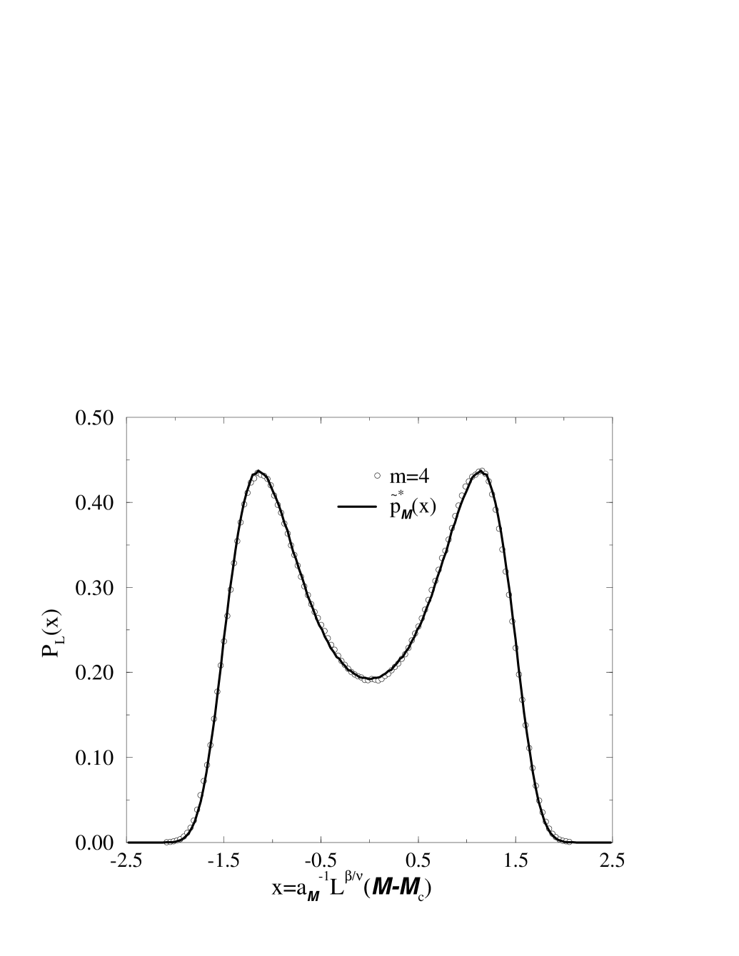
FIG. 1.: The measured form of the ordering operator distribution $p_{L}({\cal M})$ for the $m=4$ system size at the apparent critical parameters $T_{c}^{\star}=1.1853,\mu_{c}^{\star}=-2.7843$. Also shown for comparison is the universal fixed point ordering operator distribution $\tilde{p}^{\star}_{\cal M}(x)$ . The data has been expressed in terms of the scaling variable $x=a_{\cal M}^{-1}L^{\beta/\nu}({\cal M}-{\cal M}_{c})$, with the value of the non-universal scale factor $a_{\cal M}^{-1}$ chosen so that the distributions have unit variance. Statistical errors do not exceed the symbol sizes.

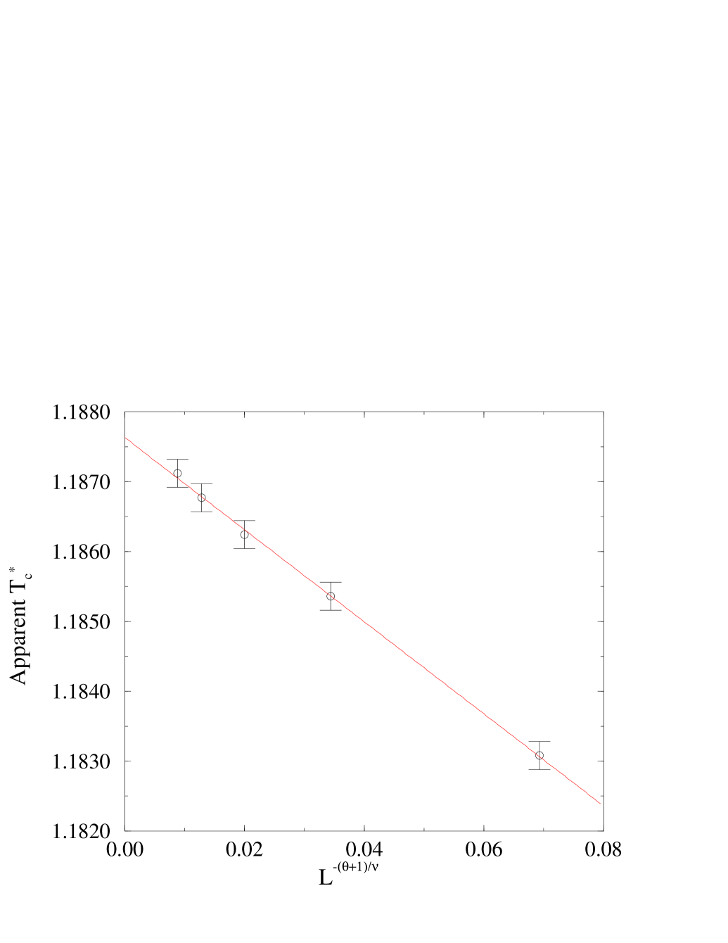
FIG. 2.: The apparent reduced critical temperature, (as defined by the matching condition described in the text), plotted as a function of $L^{-(\theta+1)/\nu}$, with $\theta=0.54$ and $\nu=0.629$[40, 47]. The extrapolation of the least squares fit to infinite volume yields the estimate $T_{c}^{\star}=1.1876(3)$.

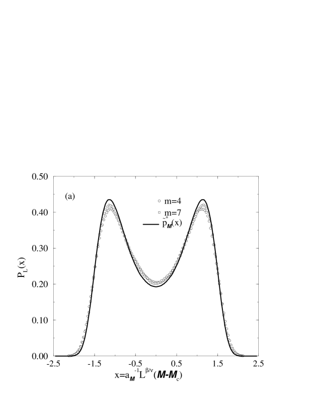
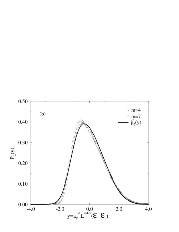
FIG. 3.: (a) The ordering operator distribution $p_{L}({\cal M})$ for the two system sizes $m=4$ and $m=7$ at the assigned critical parameters $T_{c}^{\star},\mu_{c}^{\star}$, expressed as function of the scaling variable $x=a_{\cal M}^{-1}L^{\beta/\nu}({\cal M}-{\cal M}_{c})$. Also shown (solid line) is the universal fixed point ordering operator distribution $\tilde{p}^{\star}_{\cal M}(x)$. (b) The energy operator distribution $p_{L}({\cal E})$ for the two system sizes $m=4$ and $m=7$ at $T_{c}^{\star},\mu_{c}^{\star}$ ,expressed as a function of the scaling variable $y=a_{\cal E}^{-1}L^{d-1/\nu}({\cal E}-{\cal E}_{c})$. Also shown (solid line) is the universal fixed point energy operator distribution $\tilde{p}^{\star}_{\cal E}(y)$ . In both cases the values of the non-universal scale factors $a_{\cal E}^{-1}$ or $a_{\cal M}^{-1}$ have been chosen to yield unit variance.

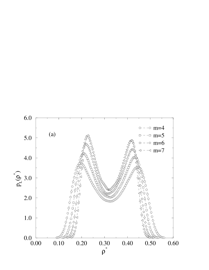
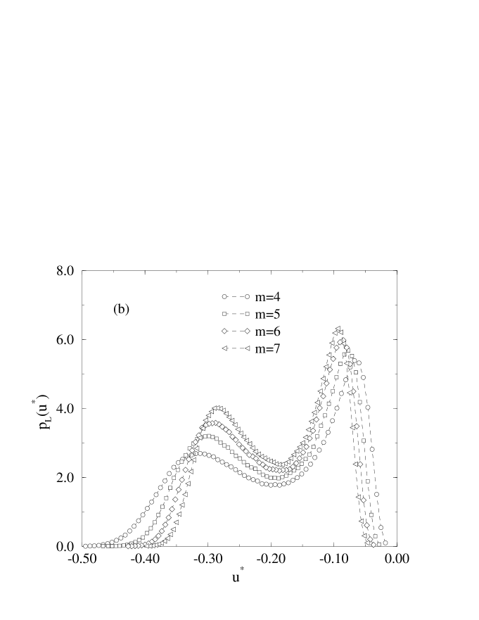
FIG. 4.: (a) The density distribution at $T_{c}^{\star},\mu_{c}^{\star}$ for the system sizes $m=4$—$7$, (b) The corresponding energy density distributions. The lines are merely guides to the eye. Statistical errors do not exceed the symbol sizes.

FIG. 5.: (a) The measured average density $\langle\rho\rangle_{c}(L)$ at the designated critical point, expressed as a function of $L^{-(d-1/\nu)}$. The least-squares fit yields an infinite volume estimate $\rho_{c}=0.3197(4)$. (b) The measured average energy density $\langle u\rangle_{c}(L)$ at the critical point, expressed as a function of $L^{-(d-1/\nu)}$ . The least-squares fit yields an infinite volume estimate $u_{c}=-0.187(2)$. In both cases we took $1/\nu=1.5887$[47].

FIG. 6.: (a) Estimates of the coexistence density distributions for the $m=4$ systems size, for a range of subcritical temperatures, obtained as described in the text. The lines are merely guides to the eye. Statistical errors do not exceed the symbol sizes.

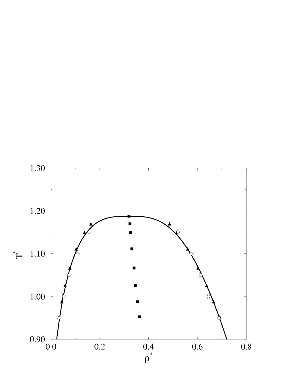
FIG. 7.: The peak densities (filled triangles) corresponding to the distributions of figure 6, plotted as a function of the reduced temperature. The coexistence diameter is also marked (filled squares). Statistical errors do not exceed the symbol sizes. Also shown (circles) are the Gibbs ensemble estimates of Panagiotopolous [43] for a system of size $L=12\sigma$. The solid line represents a fit through $T_{c}^{\star},\rho_{c}^{\star}$ of the form $\rho_{\pm}-\rho_{c}=a|T^{\star}-T_{c}^{\star}|\pm b|T^{\star}-T^{\star}_{c}|^{\beta}$, with $a=0.1824(3)$, $b=0.5226(4)$ and $\beta=0.3258\;$ [47].

FIG. 8.: The line of liquid–vapour phase coexistence in the space of $\mu^{\star}$ and $T^{\star}$, for temperatures in the range $0.95\leq T^{\star}\leq T_{c}^{\star}$. The results were obtained by implementing the equal peak weight criterion for the density distribution [49] in conjunction with the multicanonical simulations and histogram reweighting. Also shown are the measured directions of the relevant scaling fields. Statistical errors do not exceed the symbol sizes.

TABLE I.: The peak densities corresponding to the coexistence curve distributions depicted in figure 6

Temperature	$\rho_{v}$	$\rho_{g}$
1.1696	0.1635(10)	0.4855(10)
1.1494	0.1375(9)	0.5155(9)
1.1111	0.1035(9)	0.5599(9)
1.0667	0.0780(9)	0.6031(9)
1.0256	0.0580(9)	0.6380(9)
0.9877	0.0445(9)	0.6665(9)
0.9412	0.0335(8)	0.6915(8)

REFERENCES

- [1] J.-P. Hansen and L. Verlet, Phys. Rev. 184, 151 (1969).
- [2] D. Levesque and L. Verlet, Phys. Rev 182, 307 (1969).
- [3] L. Verlet and J.-J. Weis, Phys. Rev. A5, 939 (1972).
- [4] D.J. Adams, Mol. Phys. 32, 647 (1976).
- [5] D.J. Adams, Mol. Phys. 37, 211 (1979).
- [6] J.J. Nicolas, K.E. Gubbins, W.B. Streett and D.J. Tildesley, Mol. Phys. 37, 1429 (1979).
- [7] A.Z. Panagiotopoulos, Mol. Phys. 61, 813 (1987).
- [8] J.E. Finn and P.A. Monson, Phys. Rev. A39, 6402 (1989); ibid 42, 2458 (1990).
- [9] B. Smit and D. Frenkel, J. Chem. Phys. 96, 5663 (1991).
- [10] B. Smit, J. Chem. Phys. 96, 8639 (1992).
- [11] A Lotfi, A. Vrabec and J. Fischer, Mol. Phys. 76, 1319 (1992).
- [12] J. K. Johnson, J.A. Zollweg and K.E. Gubbins, Mol. Phys. 78, 591 (1993).
- [13] C. Caccamo, P.V. Giaquinta and G. Giunta, J. Phys. Condens. Matter 5, B75 (1993).
- [14] L. Reatto, A. Meroni and A. Parola, J. Phys. Condens. Matter 2, SA121 (1990).
- [15] A. Parola and L. Reatto, Phys. Rev. A31, 3309 (1985).
- [16] For a review see A.Z. Panagiotopoulos, Mol. Simul. 9, 1 (1992).
- [17] N.B. Wilding and A.D. Bruce, J. Phys. Condens. Matter 4, 3087 (1992).
- [18] K.K. Mon and K. Binder, J. Chem. Phys. 96, 6989 (1992).
- [19] M.P. Allen in Computer simulation in chemical physics, M.P. Allen and D.J. Tildesley (eds), Kluwer, Dordrecht (1993).
- [20] J.R. Recht and A.Z. Panagiotopoulos, Mol. Phys. 80, 843 (1993);
- [21] For a review, see V. Privman (ed.) Finite size scaling and numerical simulation of statistical systems (World Scientific, Singapore) (1990).
- [22] K. Binder in Computational Methods in Field Theory H. Gausterer, C.B. Lang (eds.) Springer-Verlag Berlin-Heidelberg 59-125 (1992).
- [23] A.D. Bruce and N.B. Wilding, Phys. Rev. Lett. 68, 193 (1992).
- [24] N.B. Wilding, Z. Phys. B93, 119 (1993).
- [25] N.B. Wilding and M. Müller, J. Chem. Phys. 102, 2562 (1995).
- [26] M. Müller and N.B. Wilding, Phys. Rev. E (in press).
- [27] A.D. Bruce, J. Phys. C14, 3667 (1981).
- [28] K. Binder, Z. Phys. B43, 119 (1981).
- [29] R. Hilfer, Z. Phys. B96, 63 (1994).
- [30] M.W. Pestak and M.H.W. Chan, Phys. Rev. B30, 274 (1984).
- [31] Närger U and Balzarani D A Phys. Rev. B42, 6651 (1990); U. Närger, J. R. de Bruyn, M. Stein and D.A. Balzarini, Phys. Rev. B39, 11914 (1989).
- [32] J.V. Sengers and J.M.H. Levelt Sengers, Ann. Rev. Phys. Chem. 37, 189 (1986).
- [33] Q. Zhang and J.P. Badiali, Phys. Rev. Lett. 67, 1598 (1991); Phys. Rev. A45, 8666 (1992).
- [34] J.F. Nicoll, Phys. Rev. A24, 2203 (1981); J.F. Nicoll and R.K.P. Zia, Phys. Rev. B23, 6157 (1981).
- [35] A.M. Ferrenberg and R.H. Swendsen, Phys. Rev. Lett. 61, 2635 (1988); A.M. Ferrenberg and R.H. Swendsen Phys. Rev. Lett. 63, 1195 (1989). R.H. Swendsen, Physica A194, 53 (1993).
- [36] B. A. Berg and T. Neuhaus, Phys. Rev. Lett. 68, 9 (1992).
- [37] W. Janke in Computer Simulations in Condensed Matter Physics VII, eds. D.P. Landau, K.K. Mon and H.B. Schüttler (Springer Verlag, Heidelberg, Berlin, 1994).
- [38] F.J. Wegner, Phys. Rev. B5, 4529 (1972).
- [39] J.J. Rehr and N.D. Mermin, Phys. Rev. A8, 472 (1973).
- [40] J.-H. Chen, M.E. Fisher and B.G. Nickel Phys. Rev. Lett 48, 630 (1982). See also B.G. Nickel and J. J. Rehr, J. Stat. Phys. 61, 1 (1990); A. Liu and M.E. Fisher J. Stat. Phys. 58, 431 (1990).
- [41] D.J. Adams, Mol. Phys. 29, 307 (1975).
- [42] M.P. Allen and D.J. Tildesley Computer simulation of liquids Oxford University Press (1987).
- [43] A.Z. Panagiotopoulos, preprint.
- [44] R. Hilfer and N.B. Wilding, J. Phys. A (in press).
- [45] D. Nicolaides and A.D. Bruce, J. Phys. A21, 233 (1988).
- [46] V. Privman and M.E. Fisher, J. Phys. A16, L295 (1983).
- [47] A.M. Ferrenberg, D.P. Landau, Phys. Rev. B44, 5081 (1991)
- [48] B.A. Berg, Personal communication.
- [49] C. Borgs, R. Kotecky, J. Stat. Phys. 60, 79 (1990), Phys. Rev. Lett 68, 1734 (1992), C. Borgs and S. Kappler, Phys. Lett. A171, 37 (1992); C. Borgs, P.E.L. Rakow and S. Kappler, J. Phys I (France) 4, 1027 (1994).
- [50] We note further that knowledge of the coexistence forms of obtained by multicanonical preweighting also, in principle, furnishes information on the interfacial surface tension. See e.g. B.A. Berg, U. Hansmann and T. Neuhaus, Z. Phys. B90, 229 (1993).
- [51] J.I. Siepmann, Mol. Phys. 70, 1145 (1990)
- [52] D. Frenkel, G.C.A.M. Mooij and B. Smit, J. Phys. Condens. Matter 3, 3053 (1992).