Spectral Statistics Beyond Random Matrix Theory.

Abstract

Using a nonperturbative approach we examine the large frequency asymptotics of the two-point level density correlator in weakly disordered metallic grains. This allows us to study the behavior of the two-level structure factor close to the Heisenberg time. We find that the singularities (present for random matrix ensembles) are washed out in a grain with a finite conductance. The results are nonuniversal (they depend on the shape of the grain and on its conductance), though they suggest a generalization for any system with finite Heisenberg time.

A great variety of physical systems are known to exhibit quantum chaos. The common examples are atomic nuclei, Rydberg atoms in a strong magnetic field, electrons in disordered metals, etc [1]. Chaotic behavior manifests itself in the energy level statistics. It was a remarkable discovery of Wigner and Dyson, that these statistics in a particular system can be approximated by those of an ensemble of random matrices (RM). Here we consider deviations from the RM theory taking an ensemble of weakly disordered metallic grains with a finite conductance $g$ as an example. The results seem to be extendible to general chaotic systems.

There are two characteristic energy scales associated with a particular system: a classical one $E_{c}$ and a quantum one. The quantum energy scale is the mean level spacing $\Delta$. In a chaotic billiard, for example, $E_{c}$ is set by the frequency of the shortest periodic orbit. Well developed chaotic behavior can take place only if $E_{c}\gg\Delta$.

In a disordered metallic grain the classical energy is the Thouless energy $E_{c}=D/L^{2}$, where $D$ is the diffusion constant, and $L$ is the system size. For a weakly disordered grain the two scales are separated by the dimensionless conductance $g=E_{c}/\Delta\gg 1$ [2]. For frequencies $\omega\ll E_{c}$ the behavior of the system becomes universal (independent of particular parameters of the system ). In this regime in the zeroth approximation the level statistics depend only on the symmetry of the system and are described by one of the RM ensembles: unitary, orthogonal or symplectic [3].

One of the conventional statistical spectral characteristics is the two-point level density correlator

$$K(\omega,x)=\langle\rho(\epsilon+\omega,\hat{H}+x\delta\hat{H})\rho(\epsilon,\hat{H})\rangle-\Delta^{-2},$$ (1)

where $\hat{H}$ is the Hamiltonian of the system, $\delta\hat{H}$ is a perturbation, $x$ is the dimensionless perturbation strength and $\rho(\epsilon,\hat{H}+x\delta\hat{H})={\rm Tr}\delta(\epsilon-\hat{H}-x\delta\hat{H})$ is the $x$-dependent density of states at energy $\epsilon$. It is convenient to introduce the dimensionless frequency $s=\omega/\Delta$ and the dimensionless two-level correlator $R(s,x)=\Delta^{2}K(\omega,x)$. Dyson [4] determined $R(s,x=0)$ for RM. For example, $R(s,o)$ in the unitary case equals to

$$R(s,0)=\delta(s)-\frac{1-\cos(2\pi s)}{2(\pi s)^{2}}$$ (2)

and is plotted in the insert in Fig. 1.

Perhaps the most striking signature of the Wigner-Dyson statistics is the rigidity of the energy spectrum [5]. Among the major consequences of this phenomenon are: a) the probability to find two levels separated by $\omega\ll\Delta$ vanishes as $\omega\to 0$; b) the level number variance in an energy strip of width $N\Delta$ is proportional to $\ln N$ rather than $N$; and c) oscillations in the correlator $R(s,0)$ in Eq. (2) decay only algebraically.

In the two level structure factor [6] $S(\tau,x)=\int^{\infty}_{-\infty}ds\exp(i\tau s)R(s,x)$ the reduced fluctuations of the level number manifest themselves in the vanishing of $S(\tau,0)$ at $\tau=0$, and the algebraic decay of the oscillations in $R(s,0)$ leads to the singularity in $S(\tau,0)$ at the Heisenberg time $\tau=2\pi$. In the unitary case, e. g.

$\displaystyle S(\tau,0)={\rm min}\{|\tau|/(2\pi),1\}.$

At $\tau\ll 2\pi$ this Dyson result was obtained by Berry [7] for a generic chaotic system by use of a semiclassical approximation. To the best of our knowledge nobody succeeded in analyzing the behavior of $S(\tau,0)$ around $\tau=2\pi$ using this formalism.

Wigner-Dyson statistics become exact in the limit $g=E_{c}/\Delta\to\infty$. We consider corrections to these statistics for finite $g$. One of the better understood systems in this respect is a weakly disordered metallic grain. For frequencies much smaller than $E_{c}$ the statistics are close to universal ones, the corrections being small as $(s/g)^{2}$ [8]. At $s\gg 1$ the monotonic part of $R(s,x)$ can be obtained perturbatively [9]

$$R_{{\rm p}}(s,x)=\Re\sum_{\mu}\frac{1}{\alpha\pi^{2}(-is+x^{2}+\epsilon_{\mu})^{2}},$$ (3)

where $\epsilon_{\mu}$ are eigenvalues (in units of $\Delta$) of the diffusion equation in the grain, $\alpha=2$ for the unitary ensemble and $\alpha=1$ for the orthogonal and symplectic ensembles [10]. At this point we can define

$$E_{c}=\epsilon_{1}\Delta/\pi^{2},{\qquad}g=\epsilon_{1}/\pi^{2},$$ (4)

where $\epsilon_{1}$ is the smallest nonzero eigenvalue. Perturbation theory allows one to determine $S(\tau,0)$ at small times $\tau\ll 1$. Since the oscillatory part of $R(s,x)$ is non-analytic in $1/s$ it can not be obtained perturbatively.

In this Letter we obtain the leading $s\gg 1$ asymptotics of $R(s,x)$ retaining the oscillatory terms and monitor how the singularity in $S(\tau,0)$ at the Heisenberg time is modified by the finite conductance $g$. We make use of the nonterturbative approach [11] that is valid for arbitrary relation between $s$ and $g$. The oscillatory part $R_{\rm osc}(s,x)\equiv R(s,x)-R_{\rm p}(s,x)$ for the unitary (${\rm u}$), orthogonal (${\rm o}$) and symplectic (${\rm s}$) cases equals to

$$R_{\rm osc}^{\rm u}(s,x) = \frac{\cos(2\pi s)}{2\pi^{2}y^{2}}P(s,x),$$ (6)

$$R_{\rm osc}^{\rm o}(s,x) = -\frac{\cos(2\pi s)}{2\pi^{4}y^{4}}P^{2}(s,x),$$ (7)

$$R_{\rm osc}^{\rm s}(s,x) = \frac{\cos(\pi s)}{2y}P(s,x)-\frac{\cos(2\pi s)}{2\pi^{4}y^{2}}P^{2}(s,x),$$ (8)

where $y^{2}=s^{2}+x^{4}$, and $P(s,x)$ is the spectral determinant of the diffusion operator

$$P(s,x)=\prod_{\mu,\epsilon_{\mu}\neq 0}\left[\left(\frac{s}{\epsilon_{\mu}}\right)^{2}+\left(1+\frac{x^{2}}{\epsilon_{\mu}}\right)^{2}\right]^{-1}.$$ (9)

Note that Eq. (3) expresses $R_{p}(s,x)$ through the Green function of this operator. Thus, regardless of the spectrum $\epsilon_{\mu}$, $R_{p}(s,x)$ and $R_{\rm osc}(s,x)$ are related:

$$R_{{\rm p}}(s,x)=\Re\frac{1}{\alpha\pi^{2}(-is+x^{2})^{2}}-\frac{1}{2\alpha\pi^{2}}\frac{\partial^{2}\ln[P(s,x)]}{\partial s^{2}}.$$ (10)

It follows from Eq. (9) that $R_{\rm osc}(s,x)$ together with $P(s,x)$ decays exponentially at $s\gg g$. As a result, the singularity in $S(\tau,0)$ at the Heisenberg time is washed out: $S(\tau,0)$ becomes analytic around $\tau=2\pi$. The scale of smoothening of the singularity is $1/E_{c}$ ( see Fig. 1). At $1\ll s\ll g$ the sum of Eq. (Spectral Statistics Beyond Random Matrix Theory. ) and Eq. (3) gives the leading high frequency asymptotics of the universal result, for $s\gg g$ it coincides with the perturbative result $R_{{\rm P}}(s,x)$ of Ref. [9].

In a closed ${\rm d}$-dimensional cubic sample (diffusion equation with Dirichlet boundary conditions) $\epsilon_{\mu}=g\pi^{2}\vec{n}^{2}$, where $\vec{n}=(n_{1},\ldots,n_{d})$ and $n_{i}$ are non-negative integers. For $s\gg g$ and $d<4$ we obtain the asymptotics $P(s,0)\to\exp\{-\pi(s/\pi g)^{d/2}/[\Gamma(d/2)d\sin(\pi d/4)]\}$. At $1\ll s\ll g$ we obtain

$$R(s,0)=-\frac{\sin^{2}(\pi s)}{(\pi s)^{2}}+\frac{\sin^{2}(\pi s)}{\pi^{2}g^{2}}\sum_{\vec{n}}\frac{1}{(\pi^{2}\vec{n}^{2})^{2}},$$ (11)

This result was shown in Ref. [8] to be valid even for $s<1$. Thus, it is natural to assume that for the unitary ensemble the sum of Eq. (6) and Eq. (3) gives the correct $g\to\infty$ asymptotics at arbitrary frequency. This is related to the absence of higher order corrections to the leading term of the perturbation theory $S(\tau,0)\propto\tau$ in the unitary case.

Now we sketch the derivation of our results. Consider a quantum particle moving in a random potential $V(\vec{r})$. The perturbation acting on the system is a change in the potential $\delta V(\vec{r})$. Both $V(\vec{r})$ and $\delta V(\vec{r})$ are taken to be white noise random potentials with variances $\langle V(\vec{r})V(\vec{r^{\prime}})\rangle=\delta(\vec{r}-\vec{r^{\prime}})/2\pi\nu\tau$ and $\langle\delta V(\vec{r})\delta V(\vec{r}^{\prime})\rangle=x^{2}\Delta\delta(\vec{r}-\vec{r^{\prime}})/(4\pi\nu)$, $\Delta\tau\ll 1$, $\langle V(\vec{r})\delta V(\vec{r}^{\prime})\rangle=0$, where $\langle\rangle$ denotes ensemble averaging and $\nu$ is the density of states per unit volume. The dimensionless perturbation strength $x^{2}$ is assumed to be of order unity.

We use the supersymmetric nonlinear $\sigma$-model introduced by Efetov [11], and follow his notations everywhere. One can show that for the system under consideration the $\sigma$-model expression for $K(\omega,x)$ is given by

$$K(\omega,x) = \left.-\frac{1}{\pi^{2}}\Re\frac{\partial^{2}}{\partial J^{2}}\int{\cal D}Q\exp(-F_{J})\right|_{J=0},$$ (13)

$$F_{J} = \frac{\pi\nu}{8}\int d\vec{r}{\rm STr}\left\{D(\nabla Q)^{2}+2i\omega\Lambda Q+iJ\Lambda kQ-\frac{x^{2}\Delta}{2}(\Lambda Q)^{2}\right\}.$$ (14)

The $8\times 8$ supermatrix $Q(\vec{r})$ obeys the nonlinear constraint $Q(\vec{r})^{2}=1$ and takes on its values on a certain symmetric space ${\bf H}={\bf G}/{\bf K}$, where ${\bf G}$ and ${\bf K}$ are groups [12]. For example, for the unitary ensemble ${\bf H}={\bf SU(1,1/2)}/{\bf SU(1/1)\otimes SU(1/1)}$ [13]. The integration measure for $Q$ in the functional integral Eq. (13) is the invariant measure on ${\bf H}$.

The hierarchy of blocks of supermatrices is as follows: advanced-retarded (A-R) blocks, fermion-boson (F-B) blocks, and blocks corresponding to time-reversal. $\Lambda={\rm diag}\{1,1,1,1,-1,-1,-1,-1\}$ is the matrix breaking the symmetry in the advanced-retarded (A-R ) space, $k={\rm diag}\{1,1,-1,-1,1,1,-1,-1\}$ is the symmetry breaking matrix in the Fermion-Boson ( F-B ) space.

The large frequency asymptotics of $K(\omega,x)$ can be obtained from Eq. (13) by use of the stationary phase method. The conventional perturbation theory corresponds to integrating over the small fluctuations of $Q$ around $\Lambda$ [11],

$$Q=\Lambda(1+iP)(1-iP)^{-1},P=\left(\begin{array}[]{cc}0&B\\ \bar{B}&0\end{array}\right),$$ (15)

where the matrix $P$ describes these small fluctuations.

$Q=\Lambda$ is not the only stationary point on ${\bf H}$. This fact to the best of our knowledge was not appreciated in the literature. The existence of other stationary points makes the basis for our main results.

It is possible to parameterize fluctuations around a point $Q_{0}$ in the form $Q=Q_{0}(1+iP_{0})(1-iP_{0})^{-1}$. Expanding the Free Energy $F_{J}$ in Eq. (14) in $P_{0}$ we would obtain the stationarity condition $\partial F_{J}/\partial P_{0}=0$. This route however is inconvenient because the parametrization of $P_{0}$ will depend on $Q_{0}$. Instead we perform a global coordinate transformation on ${\bf H}$ that maps $Q_{0}$ to $\Lambda$, $Q_{0}\rightarrow T_{0}^{-1}Q_{0}T_{0}=\Lambda$. We note that the matrices $\Lambda$ and $-\Lambda k$ belong to ${\bf H}$, and the corresponding terms in Eq. (14) can be viewed as symmetry breaking sources. This transformation changes the sources, but allows us to keep the parametrization of Eq. (15) and preserves the invariant measure. Introducing the notation $Q_{\Lambda}=T_{0}^{-1}\Lambda T_{0}$ and $Q_{\Lambda k}=T_{0}^{-1}\Lambda kT_{0}$ we rewrite Eq. (Spectral Statistics Beyond Random Matrix Theory. ) as

$$K(\omega,x) = \frac{\nu^{2}}{64}\Re\int{\cal D}Q\int d\vec{r}\int d\vec{r}^{\prime}{\rm STr}\Big{(}Q_{\Lambda k}Q(\vec{r})\Big{)}{\rm Str}\Big{(}Q_{\Lambda k}Q(\vec{r}^{\prime})\Big{)}\exp\left(-F(Q_{\Lambda})\right),$$ (16)

$$F(Q_{\Lambda}) = \frac{\pi\nu}{8}\int d\vec{r}{\rm STr}\left\{D(\nabla Q)^{2}+2i\omega Q_{\Lambda}Q-\frac{x^{2}\Delta}{2}(Q_{\Lambda}Q)^{2}\right\}.$$ (17)

The stationarity condition $\left.\partial F(Q_{\Lambda})/\partial P\right|_{P=0}=0$ implies that all the elements of $Q_{\Lambda}$ in the AR and RA blocks should vanish (this can be seen from Eq. (15)).

Here we discuss in detail only the calculation for the unitary ensemble. The calculation for the other cases proceeds analogously, and we just point out the important differences from the unitary case.

Consider now the unitary case. The $4\times 4$ supermatrices $B$ and $\bar{B}$ in Eq. (15) are given by

$\displaystyle B=\left(\begin{array}[]{cccc}a&0&i\sigma_{1}&0\\ 0&a^{*}&0&-i\sigma_{1}^{*}\\ \sigma_{2}^{*}&0&ib&0\\ 0&\sigma_{2}&0&ib^{*}\end{array}\right),\bar{B}=\left(\begin{array}[]{cccc}a^{*}&0&-\sigma_{2}&0\\ 0&a&0&\sigma_{2}^{*}\\ -i\sigma_{1}^{*}&0&ib^{*}&0\\ 0&-i\sigma_{1}&0&ib\end{array}\right),$

where $a$, $b$ and their conjugates are ordinary variables, and $\sigma_{1}$, $\sigma_{2}$ and their conjugates are grassmann variables.

The only matrix besides $\Lambda$ that satisfies the stationarity condition is $Q_{\Lambda}=\tilde{\Lambda}=-k\Lambda$. In this case $Q_{\Lambda k}=-\Lambda$. All other matrices from ${\bf H}$ contain nonzero elements in the AR and RA blocks. Both stationary points contribute substantially to $K(\omega,x)$.

Consider the contribution of $Q_{\Lambda}=\tilde{\Lambda}$ to $K(\omega,x)$ first. We substitute $Q_{\Lambda}=-k\Lambda$ and $Q_{\Lambda k}=-\Lambda$ into Eq. (17) and expand both the Free Energy $F(Q_{\Lambda})$ and the pre-exponent to the second order in $B$ and $\bar{B}$. Expanding $B(\vec{r})$ in the eigenfunctions of the diffusion operator $\phi_{\mu}(\vec{r})$ as $B(\vec{r})=\sum_{\mu}\phi_{\mu}(\vec{r})B_{\mu}$, and introducing ${\cal E}_{\mu}=is+\epsilon_{\mu}+x^{2}$ we arrive at the following expression for the dimensionless density-density correlator:

$$R^{\rm u}_{\rm osc}(s,x) = \Re\int{\cal D}B_{\mu}\Big{(}\sum_{\mu}[|a_{\mu}|^{2}+|b_{\mu}|^{2}-\sigma_{1,\mu}^{*}\sigma_{1,\mu}+\sigma_{2,\mu}^{*}\sigma_{2,\mu}]\Big{)}^{2}$$ (18)

$$\times \exp(-2\pi\{-is+\sum_{\mu}[{\cal E}_{\mu}|a_{\mu}|^{2}+{\cal E}^{*}_{\mu}|b_{\mu}|^{2}-\Re{\cal E}_{\mu}(\sigma_{1,\mu}^{*}\sigma_{1,\mu}-\sigma_{2,\mu}^{*}\sigma_{2,\mu})]\}).$$ (19)

We have to keep the perturbation strength $x^{2}$ finite to avoid the divergence of the integral over $a_{0}$ caused by the presence of the infinitesimal imaginary part in $\omega$. For the non parametric case we should take the $x^{2}\to 0$ limit after the integral in Eq. (19) is evaluated.

Since the Free Energy in Eq. (19) contains no Grassmann variables in the zero mode they have to come from the pre-exponent. Therefore out of the whole square of the sum in the pre-exponent only the terms containing all four zero mode Grassmann variables contribute. In these terms the prefactor does not contain any variables from non-zero modes. Thus, the evaluation of the Gaussian integrals over non-zero modes yields the superdeterminant of the quadratic form in the exponent. Supersymmetry around $\tilde{\Lambda}$ is broken by $s$, therefore this superdeterminant differs from unity and is given by $P(s,x)$ of Eq. (9). The correctly ordered integration measure for Grassmann variables is $\prod_{\mu}d\sigma_{1\mu}d\sigma_{1\mu}^{*}d\sigma_{2\mu}^{*}d\sigma_{2\mu}$. Evaluating the integral we arrive at Eq. (6).

In quasi-1D for closed boundary conditions and $x=0$ the spectral determinant $P(s,0)$ can be evaluated exactly, and from Eq. (6) we obtain

$$R^{\rm u,osc}_{1D}(s,0)=\frac{s}{2g\pi^{2}s^{2}}\frac{\cos(2\pi s)}{\sinh^{2}\left(\sqrt{\frac{s}{2g}}\right)+\sin^{2}\left(\sqrt{\frac{s}{2g}}\right)}.$$ (20)

For $Q_{\Lambda}=\Lambda$ the same procedure as used above leads to Eq. (3), which coincides with the result of Ref. [9].

The behavior of $S(\tau,0)$ at $\tau=0$ and $\tau=2\pi$ is associated respectively with $R_{\rm p}(s,0)$ (Eq. (3)) and $R^{\rm u}_{\rm osc}(s,0)$ (Eq. (6)). In other words the singularity at the Heisenberg time is determined by the contribution to $R(s,0)$ from ${\tilde{\Lambda}}$. It is clear that the cusp in $S(\tau,0)$ at $\tau=2\pi$ will be rounded off because $R^{\rm u}_{\rm osc}(s,0)$ decays exponentially at large $s$. The scale of the smoothening is of order $1/g$.

The Fourier transform of Eq. (20) ( see Fig. 1 ) is

$$S^{\rm u}_{1D}(2\pi+t,0)_{\tilde{\Lambda}}=\sum_{n=1}^{\infty}\frac{(-1)^{n}\exp(-\pi^{2}n^{2}g|t|)}{\pi^{2}gn\sinh(\pi n)}-\frac{|t|}{4\pi}.$$ (21)

Even though $S^{\rm u}_{1D}(2\pi+t,0)_{\tilde{\Lambda}}$ appears to be a function of $|t|$, it is regular at $t=0$.

We can also estimate $S^{\rm u}(2\pi,0)_{\tilde{\Lambda}}$ in any dimension. It is proportional to $1/g$ of Eq. (4) and is given by

$\displaystyle S^{\rm u}(2\pi,0)_{\tilde{\Lambda}}=\frac{1}{4\pi^{4}g}\int_{-\infty+i\eta}^{\infty+i\eta}\frac{dz}{z^{2}}\prod_{\mu\epsilon_{\mu}\neq 0}\left(1+\left[\frac{z\epsilon_{1}}{\epsilon_{\mu}}\right]^{2}\right)^{-1}.$

Consider now T-invariant systems. For the orthogonal ensemble there are still only two stationary points on ${\bf H}$: $\Lambda$ and $\tilde{\Lambda}=-k\Lambda$. To determine the contribution of the $\tilde{\Lambda}$-point we use the formula Eq. (17) with $Q_{\Lambda}=\tilde{\Lambda}$ and $Q_{k\Lambda}=-\Lambda$ and Efetov’s parametrization for the perturbation theory [11]. The calculations are analogous to those for the unitary ensemble and lead to Eq. (7). The contribution of $Q_{\Lambda}=\Lambda$ gives Eq. (3). At $\tau=2\pi$ the third derivative of $S(\tau,0)$ for the orthogonal ensemble has a jump. This singularity also disappears at finite $g$.

In the symplectic case there are three types of stationary points which correspond to singularities in the structure factor $S(\tau,0)$ at $\tau=0,\pi,2\pi$ [3]. The $\tau=2\pi$ singularity corresponds to $Q_{\Lambda}=\tilde{\Lambda}=-k\Lambda$, and its contribution to $R(s,x)$, given by the second term in Eq. (8), is exactly the same as $R^{\rm o}_{\rm osc}(s,x)$. The stationary point $Q_{\Lambda}=\Lambda$ corresponds to the $\tau=0$ singularity in $S(\tau,0)$ and leads to Eq. (3). The $\tau=\pi$ singularity corresponds to a degenerate manifold of matrices $Q_{\Lambda}$ on ${\bf H}$ $Q_{\Lambda}={\rm diag}(\tau_{\vec{m}},\openone_{2},-\tau_{\vec{m}},-\openone_{2})$, $Q_{k\Lambda}=-kQ_{\Lambda}$, where ${\openone_{2}}$ is a $2\times 2$ unit matrix, $\tau_{\vec{m}}=m_{x}\tau_{x}+m_{y}\tau_{y}$, $\vec{m}^{2}=1$ and $\tau_{x,y}$ are Pauli matrices in the time-reversal block. The calculation proceeds as before and leads to the first term in Eq. (8). In quasi-1D we can obtain the leading contribution to the structure factor $S(\tau,0)$ around $\tau=\pi$

$$S^{\rm s}(t+\pi,0)=\int_{0}^{\infty}\frac{-4\sin^{2}(g|t|z)dz}{\sinh^{2}\sqrt{z}+\sin^{2}\sqrt{z}}+\ln(1.9g)+O(1/g).$$ (22)

The result is plotted in Fig. 2. In all dimensions the logarithmic divergence in the zero mode result is now cut off by finite $g$, and $S^{\rm s}(\pi,0)\propto\ln g$.

In conclusion we mention several points about our results. 1) Equation (Spectral Statistics Beyond Random Matrix Theory. ) describes the deviation of the level statistics of a weakly disordered chaotic grain from the universal ones. This deviation is controlled by the diffusion operator. This operator is purely classical. It seems plausible that the nonuniversal part of spectral statistics of any chaotic system can be expressed through a spectral determinant of some classical system-specific operator. If so, the relation Eq. (10) should be universally correct!

2) The formalism used here should be applicable even to the systems weakly coupled to the outside world (say through tunnel contacts). As long as the level broadening $\Gamma$ ($\omega=\Re\omega+i\Gamma$) is smaller than $\Delta x^{2}$ the integration over the zero mode variables in Eq. (19) is convergent. The integral over the other modes is always convergent provided $\Gamma<E_{c}$. Thus, the presence of a perturbation can effectively “close” a weakly coupled system. Under these conditions Eq. (Spectral Statistics Beyond Random Matrix Theory. ) remains valid after the substitution $\cos(2\pi s)\to\exp(-2\pi\Gamma/\Delta)\cos(2\pi s)$ and $x^{2}\to x^{2}-\Gamma/\Delta$.

3) The classification of physical systems into the three universality classes (unitary, orthogonal and symplectic) is, of course, an oversimplification. In practice there is always a time scale which determines the crossover from one ensemble to another. For example if a system is subjected to a magnetic field for very short times it will still effectively remain orthogonal. On the other hand, the long time behavior will be unitary. The characteristic time is set by the strength of the magnetic field.

For a disordered metallic grain in a magnetic field this characteristic time is given by $l^{2}_{H}/D$. For frequencies larger than $D/l^{2}_{H}$ the system effectively becomes orthogonal. This implies that even if we neglect the spatially nonuniform fluctuations of the $Q$-matrix the cusp in $S(\tau,0)$ at $\tau=2\pi$ will be washed out on the scale of $\Delta l_{H}^{2}/D$ ( although there will still remain a jump in the third derivative of $S(\tau,0)$ ). For the system to behave as unitary for frequencies of order $E_{c}$ the magnetic length $l_{H}$ has to be shorter than the size of the system. Spin-orbit interaction that causes the orthogonal-to-symplectic crossover can be considered in a similar way.

4) The rounding off of the singularity in $S(2\pi,0)$ is also present in the random matrix model with preferred basis [14] [15]. Note that our results differ from those in Ref. [15] substantially. This means that finite $g$ is not equivalent to finite temperature for the corresponding Calogero-Sutherland model [16].

We are grateful to D. E. Khmel’nitskii, B. D. Simons and N. Taniguchi for numerous discussions throughout the course of this work.

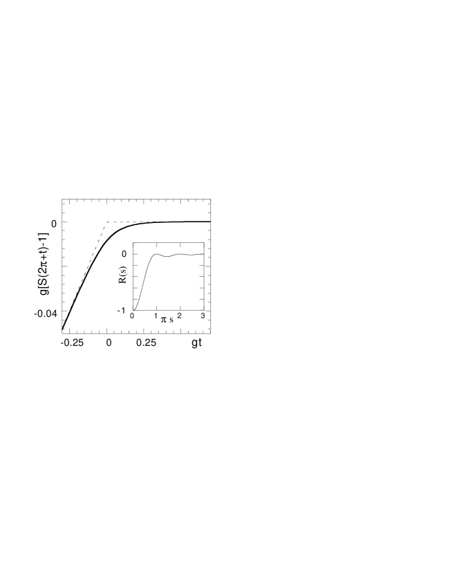
FIG. 1.: Structure factor in quasi-1D case for unitary symmetry (solid line) and the universal structure factor (dashed line). Insert: the two level correlator as a function of level separation.

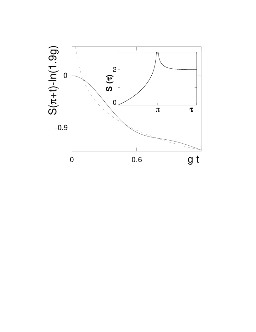
FIG. 2.: The structure factor for the symplectic case in quasi-1D (solid line) and the universal result (dashed line). Insert: the universal stucture factor.

REFERENCES

- [1] Chaos in Quantum Physics, eds., M. J. Jianonni, A. Voros and J. Zinn-Justin, Les Houches, Session LII 1989 (North-Holland, Amsterdam, 1991)
- [2] D. J. Thouless, Phys. Rep. 13, 93 (1974)
- [3] M. L. Mehta, Random Matrices, (Academic Press, New York, 1991)
- [4] F. J. Dyson, J. Math. Phys. 3, 140, 157, 166 (1962)
- [5] F. Haake, Quantum Signatures of Chaos (Springer, Berlin, 1991)
- [6] The function , for example, describes the phenomenon of “quantum echo” in mesoscopic quantum dots. See V. N. Prigodin et al, Phys. Rev. Lett. 72, 546 (1994)
- [7] M. V. Berry, Proc. Roy. Soc. London A 400, 229 (1985)
- [8] V. E. Kravtsov, A. D. Mirlin, Sov. Phys. JETP Lett., 60, 656 (1994). [Pis’ma ZhETF, 60, 645 (1994) ]
- [9] B. L. Altshuler, B. I. Shklovskii, JETP 64, 127 (1986).
- [10] This definition of is related to the fact that for the unitary and orthogonal cases is the mean level spacing per spin polarization, and for the symplectic case it is one-half of that.
- [11] K. B. Efetov Adv. Phys. 32, 53 (1983).
- [12] J. J. Verbaarscot, H. A. Weidenmuller, M. R. Zirnbauer, Phys. Rep. 129, 367 (1985)
- [13] M. R. Zirnbauer, Nucl. Phys.B [FS] 265, 375 (1986)
- [14] J. -L. Pichard, B. Shapiro J. Phys. May(1994)
- [15] M. Moshe, H. Neunberger, B. Shapiro, preprint RU-94-28, Technion PH-12-94 (1994)
- [16] B. D. Simons, P. A. Lee and B. L. Altshuler, Nucl. Phys.B 409, 487 (1993)