Infrared conductivity in layered $d$-wave superconductors

Abstract

We calculate the infrared conductivity of a stack of coupled, two-dimensional superconducting planes within the Fermi liquid theory of superconductivity. We include the effects of random scattering processes and show that the presence of even a small concentration of resonant impurities, in a $d$-wave superconductor, has an important effect on both the in-plane and $c$-axis transport properties, which could serve as signatures for $d$-wave pairing.

I INTRODUCTION

One of the central issues in the field of high temperature superconductivity is the symmetry of the superconducting order parameter. A number of recent experiments, specifically Josephson interference experiments, suggest a $d$-wave order parameter with $d_{x^{2}-y^{2}}$ symmetry,[2, 3, 4, 5] while experiments on $c$-axis tunneling[6] are consistent with a traditional $s$-wave order parameter. In this paper we calculate the in-plane and $c$-axis conductivities for layered, $d$-wave superconductors in the limit $q\to 0$ and for frequencies $\hbar\omega\sim\Delta$ (infrared region). This long wavelength regime is appropriate for superconductors with a mean free path that is short compared to the penetration length, $\ell\ll\lambda$. Given the small coherence length in cuprates, the $q\to 0$ limit for the conductivity easily accommodates the clean limit condition, $\xi\ll\ell$, which is necessary for $d$-wave superconductivity not to be suppressed. Calculations of the conductivity in the ultraclean limit ($\ell\gg\lambda\gg\xi$), which include polarization sensitivity to the in-plane absorption and vertex corrections to the conductivity from collective modes, will be discussed in a separate paper.

In order to represent the layered structure of high-$T_{c}$ superconductors, we consider the microscopic model of coupled superconducting layers introduced in Ref. [7]. In this model the charge carriers of each layer form a two-dimensional Fermi liquid, which we describe by the quasiclassical theory of superconductivity. Thus, in-plane transport is dominated by charged quasiparticles moving with an in-plane Fermi velocity, ${\bf v}_{f}$. Interlayer transport may originate from coherent propagation,[8, 9, 10, 11, 12] static and thermally activated (e.g., phonon assisted or pair fluctuation) incoherent charge transfer,[7, 8, 13, 14] resonant transfer,[15] or several transfer mechanisms in parallel.[16, 17, 18, 19, 20, 21] Interlayer transport has also been argued to take place through coherent pair tunneling.[22] In this report we consider a model in which the interlayer coupling is mediated through incoherent hopping processes (the interlayer diffusion model), as in Ref. [7]. These incoherent scattering events are predominantly responsible for charge transfer in the $c$ direction and Josephson coupling between the planes. For simplicity, we consider a circular Fermi surface for each conducting layer. This model is expected to be appropriate for superconductors whose $c$-axis behavior is that of a stack of superconductor-insulator-superconductor ($SIS$) Josephson junctions. Such behavior has recently been observed experimentally in several layered superconducting compounds. [23, 24, 25, 26]

The infrared conductivity of three-dimensional bulk superconductors with unconventional pairing has been calculated previously by Klemm et al.,[27] Hirschfeld et al.,[28] and for two-dimensional superconductors by Hirschfeld, Putikka and Scalapino [29] using Green function methods; our results agree with those found previously whenever a direct comparison is possible. We calculate the infrared conductivity for layered superconductors and find striking differences between the conductivities of the $d$-wave and $s$-wave models. These differences between $s$-wave and $d$-wave conductivities are not due just to the differences in the density of states, which are known to lead to different low-temperature behavior of the penetration depth, NMR relaxation rates, etc.[30] There are additional features in the conductivity of $d$-wave superconductors which are attributed to the formation of optically active Andreev bound states.

The outline of this paper is the following. In Sec. II, we present our microscopic model in terms of the Fermi liquid theory of superconductivity. Then in Sec. III we formulate the linear current response to a spatially homogeneous, electromagnetic perturbation. Section IV includes a discussion of the phenomenological parameters of our model as well as the results of the current response calculations. We relate the model parameters to measurable normal-state quantities and calculate properties of the superconducting state for both $s$-wave and $d$-wave pairing interactions. We discuss the consistency between these two models and experiments, and discuss the results of the linear response calculations of the in-plane and $c$-axis infrared conductivities.

II QUASICLASSICAL THEORY

We perform the calculations within the quasiclassical theory of superconductivity, first developed by Eilenberger,[31] Larkin and Ovchinnikov,[32] and Eliashberg.[33] This theory is capable of describing both the equilibrium and dynamical properties of a Fermi liquid, in either the normal or superconducting state. We briefly outline the basic equations of this theory without discussing their justification; readers interested in these details should see the original papers mentioned above, or the recent review articles.[34, 35, 36, 37, 38] We follow closely the notation of Refs. [7] and [34]. In this report we are interested in the linear response of a homogeneous, superconducting Fermi liquid to an electric field described by a spatially uniform, time-dependent vector potential. With this in mind, we start from the basic equations of the quasiclassical theory neglecting the dependence on the space coordinate (${\bf R}$).

A Basic Equations

The most fundamental quantity in the quasiclassical theory of superconductivity is the matrix propagator for quasiparticle excitations. In order to describe nonequilibrium properties we use Keldysh’s formulation of dynamical phenomena (see Appendix).[39] This technique requires three types of propagators: retarded, $\hat{g}^{R}$, advanced, $\hat{g}^{A}$, and Keldysh, $\hat{g}^{K}$. These propagators are $2\times 2$ matrices in particle-hole (Nambu) space,

$${\hat{g}}^{R,A,K}\left(s;\epsilon,t\right)=\left(\begin{array}[]{cc}g^{R,A,K}&f^{R,A,K}\\ \bar{f}^{R,A,K}&\bar{g}^{R,A,K}\end{array}\right).$$ (1)

Note that we are limiting our considerations to distribution functions which are spin scalars only; a more complete description of this theory, including spin-dependent effects, can be found elsewhere.[34] For a spatially homogeneous Fermi liquid, the propagators $\hat{g}^{R,A,K}\left(s;\epsilon,t\right)$ are functions of the Fermi surface position, $s$, the single particle excitation energy, $\epsilon$, and time, $t$. Their diagonal components are related to the spectrum and distribution of Bogoliubov quasiparticle excitations, while their off-diagonal components yield the Cooper-pair amplitude. In principle, $\hat{g}^{K}$ contains all of the information about the relevant measurable quantities (equilibrium and dynamic) in both the normal and superconducting states. We make use of a compact notation which combines the three Nambu matrices, $\hat{g}^{R,A,K}$, into a single Nambu-Keldysh matrix,

$${\hat{g}}\left(s;\epsilon,t\right)=\left(\begin{array}[]{cc}{\hat{g}}^{R}&{\hat{g}}^{K}\\ 0&{\hat{g}}^{A}\end{array}\right).$$ (2)

Thus, any operator written without superscript (e.g., $\hat{a}$) is interpreted as a Nambu-Keldysh matrix, while its retarded, advanced, and Keldysh Nambu-matrix components are denoted by the appropriate superscripts (e.g., $\hat{a}^{R,A,K}$).

The central equation of the Fermi liquid theory of superconductivity is the quasiclassical transport equation

$$\displaystyle\left[\left(\epsilon+\frac{e}{c}{\bf v}_{f}\cdot{\bf A}_{\ell}\right){\hat{\tau}}_{3}-e\Phi_{\ell}\hat{1}-\hat{\Delta}_{\ell}-\mbox{$\hat{\mbox{$\Sigma$}}$}_{\ell}\,,\,\hat{g}_{\ell}\right]_{\otimes}=0,$$ (3)

supplemented by the normalization condition

$$\hat{g}_{\ell}\otimes\hat{g}_{\ell}=-\pi^{2}\hat{1}.$$ (4)

The $\hat{\tau}_{3}$ in equation (3) is to be understood as the third Pauli matrix in particle-hole space combined with the unit matrix in Keldysh space. Equation (3) generalizes the Landau-Boltzmann transport equation for normal Fermi liquids to the superconducting state. In our model we have a transport equation for each layer, specified by the discrete index $\ell$. The spectrum and distribution of quasiparticles in layer $\ell$ are affected by the in-plane vector potential, ${\bf A}_{\ell}(t)$, the scalar potential, $\Phi_{\ell}(t)$, the pairing field, $\hat{\Delta}_{\ell}(s,t)$, and the scattering self-energy, $\mbox{$\hat{\mbox{$\Sigma$}}$}_{\ell}(s;\epsilon,t)$. The coupling of quasiparticles (of charge $e$) to an electromagnetic field appears explicitly in equation (3), and also implicitly through the field dependence of the self-energy, $\mbox{$\hat{\mbox{$\Sigma$}}$}_{\ell}$. The Fermi velocity, ${\bf v}_{f}$, is a two-dimensional vector parallel to the planes. The commutator in equation (3) is defined as $[\hat{a},\hat{b}]_{\otimes}=\hat{a}\otimes\hat{b}-\hat{b}\otimes\hat{a}$, where the symbol $\otimes$ denotes a folding product in the energy-time domain (see Appendix), together with matrix multiplication of Nambu-Keldysh matrices. For details of this formalism see Refs. [34, 35, 36, 37, 38].

In the weak-coupling approximation, the retarded, advanced, and Keldysh components of the pairing field take the form

$$\hat{\Delta}_{\ell}^{R,A}\left(s;t\right)=\int\frac{d\epsilon}{4\pi i}\left<V\left(s,s^{\prime}\right)\hat{f}^{K}_{\ell}\left(s^{\prime};\epsilon,t\right)\right>_{s^{\prime}},$$ (5)

$$\hat{\Delta}_{\ell}^{K}\left(s;t\right)=0.$$ (6)

Here $V(s,s^{\prime})$ is the pairing interaction, which determines both $T_{c}$ and the symmetry of the order parameter, and $\hat{f}^{K}$ denotes the off-diagonal part of the Keldysh propagator, $\hat{g}^{K}$. The notation $\left<F(s)\right>_{s}$ denotes a Fermi surface average, $\int d^{2}s\,n(s)F(s)$, where $n(s)$ describes the local density of quasiparticle states on the Fermi surface, normalized so that $\int d^{2}s\,n(s)=1$. For the case of isotropic $s$-wave pairing, the pairing interaction takes the form $V\left(s,s^{\prime}\right)=V_{0}$, while for a $d$-wave model, $V\left(s,s^{\prime}\right)$ favors a pairing field with $d_{x^{2}-y^{2}}$ symmetry, although essentially all of the results presented here are valid for any unconventional order parameter with line nodes on the two-dimensional Fermi surface.

The scattering self-energy of layer $\ell$, $\mbox{$\hat{\mbox{$\Sigma$}}$}_{\ell}=\mbox{$\hat{\mbox{$\Sigma$}}$}^{\|}_{\ell}+\mbox{$\hat{\mbox{$\Sigma$}}$}^{\bot}_{\ell,\ell-1}+\mbox{$\hat{\mbox{$\Sigma$}}$}^{\bot}_{\ell,\ell+1}$, describes both in-plane scattering ($\mbox{$\hat{\mbox{$\Sigma$}}$}^{\|}_{\ell}$) and interplane scattering ($\mbox{$\hat{\mbox{$\Sigma$}}$}^{\bot}_{\ell,\ell\pm 1}$). In-plane scattering processes are taken into account via a self-energy of the form

$$\mbox{$\hat{\mbox{$\Sigma$}}$}^{\|}_{\ell}\left(s;\epsilon,t\right)=c_{i}\,\hat{t}_{\ell}\left(s,s;\epsilon,t\right),$$ (7)

where $c_{i}$ is an effective concentration of scattering centers. We consider isotropic in-plane scattering, in which case $\hat{u}_{0}=u_{0}\,\hat{1}$ is an isotropic scattering potential. The $s$-dependence drops out of the in-plane $\hat{t}$ matrix so that

$$\hat{t}_{\ell}\left(\epsilon,t\right)=\hat{u}_{0}+\hat{u}_{0}\otimes\left[N_{f}\left<\hat{g}_{\ell}\left(s;\epsilon,t\right)\right>_{s}\right]\otimes\hat{t}_{\ell}\left(\epsilon,t\right),$$ (8)

where $N_{f}$ is the density of states at the Fermi energy. The scattering self-energy, $\mbox{$\hat{\mbox{$\Sigma$}}$}^{\|}_{\ell}$, then contains only two independent parameters. Following Buchholtz and Zwicknagl,[40] we choose these two parameters to be the normal-state scattering rate,

$$\frac{\hbar}{\tau_{\|}}=\frac{2\pi c_{i}N_{f}u_{0}^{2}}{1+\left(N_{f}u_{0}\pi\right)^{2}},$$ (9)

and the normalized scattering cross section,

$$\bar{\sigma}=\frac{\left(N_{f}u_{0}\pi\right)^{2}}{1+\left(N_{f}u_{0}\pi\right)^{2}}\,,$$ (10)

which is the true cross section divided by the cross section in the unitarity limit, $\sigma^{(u)}_{2d}=4/k_{f}$. Thus, the normalized cross section ranges from $\bar{\sigma}=0$ for weak scattering (Born limit), to $\bar{\sigma}=1$ for strong scattering (unitarity limit). We have formulated the in-plane scattering self-energy in terms of a $\hat{t}$ matrix. In this formulation, the self-energy covers impurity scattering, including resonant scattering, as well as any other type of scattering process, elastic or inelastic, as long as it can be approximated by an effective lifetime and an effective cross section. For instance, electron-phonon scattering in this approximation corresponds to $\bar{\sigma}=0$ (Migdal’s theorem) and a temperature dependent lifetime, $\tau_{||}(T)$.

Since we neglect coherent transport along the $c$-axis (i.e., we set the Fermi velocity along the $c$-axis to zero), the interlayer scattering self-energies, $\mbox{$\hat{\mbox{$\Sigma$}}$}^{\bot}_{\ell,\ell\pm 1}$, are the only source of interlayer coupling in the model. We assume this coupling to be weak (nonresonant), and thus describe interlayer scattering by a self-energy in the Born approximation,

$$\mbox{$\hat{\mbox{$\Sigma$}}$}^{\bot}_{\ell,\ell\pm 1}(s;\epsilon,t) = {\hat{U}}_{\ell,\ell\pm 1}(t)\otimes\left[\frac{\hbar}{2\pi}\left\langle\frac{1}{\tau_{\bot}(s,s^{\prime})}\,{\hat{g}}_{\ell\pm 1}(s^{\prime};\epsilon,t)\right\rangle_{\!\!\!s^{\prime}}\right]\otimes{\hat{U}}^{\dagger}_{\ell,\ell\pm 1}(t)\ .$$ (11)

The interlayer self-energy is parametrized by an effective lifetime, $\tau_{\bot}$, which is the characteristic time between consecutive scattering processes between layers.[41] The gauge operators, ${\hat{U}}_{\ell,\ell\pm 1}$, and interlayer vector potentials, $A^{z}_{\ell,\ell\pm 1}$, are defined by

$${\hat{U}}_{\ell,\ell\pm 1}(t) = \exp\left(-i\frac{ed}{\hbar c}A^{z}_{\ell,\ell\pm 1}(t){\hat{\tau}}_{3}\right),$$ (12)

$$A^{z}_{\ell,\ell\pm 1}(t) = \frac{1}{d}\int_{\ell\cdot d}^{(\ell\pm 1)\cdot d}dzA^{z}(z,t),$$ (13)

where $d$ is the layer spacing. The effective interlayer scattering lifetime, $\tau_{\bot}(s,s^{\prime})$, is generally anisotropic. We describe this anisotropy by

$$\frac{1}{\tau_{\bot}(s,s^{\prime})}=\frac{1}{\tau_{\bot}}\frac{\exp\left[\gamma\,\cos{\left(\varphi(s)-\varphi(s^{\prime})\right)}\right]}{\langle\langle\exp\left[\gamma\,\cos{\left(\varphi(s)-\varphi(s^{\prime})\right)}\right]\rangle_{s}\rangle_{s^{\prime}}}.$$ (14)

The real space angles $\varphi(s)$ and $\varphi(s^{\prime})$ give the in-plane directions of the quasiparticle Fermi velocity before and after scattering to an adjacent layer. The parameter $\gamma$ specifies to what degree the scattered electrons “remember” their initial momentum. Isotropic scattering corresponds to $\gamma=0$, while extreme forward scattering corresponds to $\gamma\to\infty$. The scattering rate is illustrated in figure (1) for several values of the parameter $\gamma$. Note that in the interlayer diffusion model one needs an anisotropic $c$-axis scattering rate to get a nonzero interlayer Josephson coupling with a $d$-wave order parameter.[41] However, higher order tunneling processes also give a nonzero Josephson coupling.[42]

Here we are concerned with the current response to a weak electric field for a layered $d$-wave superconductor. The in-plane current is carried by quasiparticles moving with an in-plane velocity ${\bf v}_{f}$, and is given by standard equations of quasiclassical theory [34, 35, 36]

$${\bf j}_{\ell}(t)=eN_{f}\int{d\epsilon\over 4\pi i}\left<{\bf v}_{f}(s)\,{\mbox{Tr}}\left[{\hat{\tau}}_{3}\,\hat{g}_{\ell}^{K}(s;\epsilon,t)\right]\right>_{s}\ .$$ (15)

The interlayer current, on the other hand, is of a different nature. It originates from random scattering processes of quasiparticles between adjacent layers. The microscopic expression for the interlayer current density was derived for isotropic interlayer scattering in Ref. [7], and is generalized below to anisotropic scattering,

$$j^{z}_{\ell,\ell+1}(t) = -\frac{eN_{f}d}{i\hbar}\int{d\epsilon\over 4\pi i}\left\langle\mbox{Tr}\left\{{\hat{\tau}}_{3}\;\Bigl{[}\mbox{$\hat{\mbox{$\Sigma$}}$}_{\ell,\ell+1}^{\bot}(s;\epsilon,t)\ ,\hat{g}_{\ell}(s;\epsilon)\Bigr{]}_{\otimes}\right\}^{K}\right\rangle_{s}$$ (16)

$$= -\frac{eN_{f}d}{i\hbar}\int{d\epsilon\over 4\pi i}\left\langle{\mbox{Tr}}\left\{{\hat{\tau}}_{3}\;\Bigl{(}\Bigr{.}\right.\right.{\mbox{$\hat{\mbox{$\Sigma$}}$}_{\ell,\ell+1}^{\bot,\,R}}\otimes{{\hat{g}}}_{\ell}^{K}+{\mbox{$\hat{\mbox{$\Sigma$}}$}_{\ell,\ell+1}^{\bot,\,K}}\otimes{{\hat{g}}}_{\ell}^{A}-{{\hat{g}}}_{\ell}^{R}\otimes{\mbox{$\hat{\mbox{$\Sigma$}}$}_{\ell,\ell+1}^{\bot,\,K}}-{{\hat{g}}}_{\ell}^{K}\otimes{\mbox{$\hat{\mbox{$\Sigma$}}$}_{\ell,\ell+1}^{\bot,\,A}}\left.\left.\Bigl{.}\Bigr{)}\right\}\right\rangle_{s}\ .$$ (17)

Equations (15) and (16) cover the current response for both normal and superconducting states, in equilibrium and nonequilibrium situations.

B Equilibrium Solution

In the absence of external perturbations, the quasiclassical transport equation and normalization condition for the equilibrium retarded and advanced propagators become

$$\left[\epsilon\hat{\tau}_{3}-\hat{\Delta}^{R,A}\left(s\right)-\mbox{$\hat{\mbox{$\Sigma$}}$}^{R,A}\left(s;\epsilon\right),\hat{g}^{R,A}\left(s;\epsilon\right)\right]=0,$$ (18)

$$\left[\hat{g}^{R,A}\left(s;\epsilon\right)\right]^{2}=-\pi^{2}\hat{1},$$ (19)

where the $\otimes$ products reduce to simple matrix multiplication. We dropped the layer index $\ell$, since all layers are equivalent in equilibrium. In the real gauge, the pairing field has the simple form, $\hat{\Delta}^{R,A}(s)=i\Delta_{0}(s)\hat{\tau}_{2}$. Choosing this gauge, we solve equations (18) and (19), and obtain

$$\hat{g}^{R,A}\left(s;\epsilon\right)=-\pi\frac{\tilde{\epsilon}^{R,A}\left(s;\epsilon\right)\hat{\tau}_{3}-i\tilde{\Delta}^{R,A}\left(s;\epsilon\right)\hat{\tau}_{2}}{\sqrt{\tilde{\Delta}^{R,A}\left(s;\epsilon\right)^{2}-\tilde{\epsilon}^{R,A}\left(s;\epsilon\right)^{2}}},$$ (20)

where the $\tilde{\epsilon}$ and $\tilde{\Delta}$ can be interpreted as the “renormalized” excitation energy and gap function due to scattering processes. The renormalized quantities are determined by the scattering self-energy, $\mbox{$\hat{\mbox{$\Sigma$}}$}^{R,A}$, and are given by

$$\tilde{\epsilon}^{R,A}\left(s;\epsilon\right) = \epsilon-{1\over 2}{\mbox{Tr}}\left[\hat{\tau}_{3}\mbox{$\hat{\mbox{$\Sigma$}}$}^{R,A}\left(s;\epsilon\right)\right],$$ (21)

$$\tilde{\Delta}^{R,A}\left(s;\epsilon\right) = \Delta_{0}\left(s\right)-{i\over 2}{\mbox{Tr}}\left[\hat{\tau}_{2}\mbox{$\hat{\mbox{$\Sigma$}}$}^{R,A}\left(s;\epsilon\right)\right].$$ (22)

The in-plane scattering self-energy can be evaluated by solving equation (8) to obtain

$$\mbox{$\hat{\mbox{$\Sigma$}}$}^{R,A}_{\|}\left(\epsilon\right)=\frac{\hbar}{2\tau_{\|}}\frac{1}{1-\bar{\sigma}\left[1+\left(\pi^{-1}\left<\hat{g}^{R,A}(s;\epsilon)\right>_{s}\right)^{2}\right]}\left[\sqrt{\frac{1}{\bar{\sigma}}-1}+\frac{\left<\hat{g}^{R,A}(s;\epsilon)\right>_{s}}{\pi}\right],$$ (23)

while the interplane self-energy has the simple form

$$\mbox{$\hat{\mbox{$\Sigma$}}$}^{R,A}_{\bot}\left(s;\epsilon\right)=\frac{\hbar}{2\pi}\left<\frac{1}{\tau_{\bot}\left(s,s^{\prime}\right)}\hat{g}^{R,A}(s^{\prime};\epsilon)\right>_{s^{\prime}}.$$ (24)

From the solutions for the equilibrium retarded and advanced propagators and self-energies, one can calculate the equilibrium Keldysh components,

$$\hat{g}^{K}\left(s;\epsilon\right)=\tanh\left(\frac{\epsilon}{2\mbox{$k_{\text{B}}$}T}\right)\left(\hat{g}^{R}\left(s;\epsilon\right)-\hat{g}^{A}\left(s;\epsilon\right)\right),$$ (25)

$$\mbox{$\hat{\mbox{$\Sigma$}}$}^{K}\left(s;\epsilon\right)=\tanh\left(\frac{\epsilon}{2\mbox{$k_{\text{B}}$}T}\right)\left(\mbox{$\hat{\mbox{$\Sigma$}}$}^{R}\left(s;\epsilon\right)-\mbox{$\hat{\mbox{$\Sigma$}}$}^{A}\left(s;\epsilon\right)\right).$$ (26)

C The $d$-wave Model

So far the presentation of the quasiclassical theory has been fairly general. To make further progress we must specify the shape of the Fermi surface and the form of the pairing interaction, $V(s,s^{\prime})$. We consider a simple model that incorporates $d$-wave pairing. We assume a cylindrical Fermi surface (in which case the Fermi surface position, $s$, is replaced by the azimuthal angle, $\phi$), and a pairing interaction of the form

$$V\left(\phi,\phi^{\prime}\right)=V_{0}\,\cos{\left(2\phi\right)}\cos{\left(2\phi^{\prime}\right)}.$$ (27)

Note that the basis functions for this pairing interaction possess the usual $k_{x}^{2}-k_{y}^{2}$ anisotropy. The angular dependences of the self-energies are now determined, and the remaining task is to solve for the magnitudes and energy dependences. For a system in equilibrium, and in the absence of any perturbations, we find from equation (5) that the pairing field has the form

$$\hat{\Delta}_{0}^{R,A}\left(\phi\right)=i\Delta_{0}\cos{\left(2\phi\right)}\hat{\tau}_{2}\,,$$ (28)

and from equation (23) the in-plane scattering self-energy becomes

$$\mbox{$\hat{\mbox{$\Sigma$}}$}^{R,A}_{\|}\left(\epsilon\right)=\frac{\hbar}{2\tau_{\|}}\frac{1}{1-\bar{\sigma}\left[1+\left(\pi^{-1}\langle g^{R,A}_{3}(\phi;\epsilon)\rangle_{\phi}\right)^{2}\right]}\left[\sqrt{\frac{1}{\bar{\sigma}}-1}+\frac{\langle g^{R,A}_{3}(\phi;\epsilon)\rangle_{\phi}\hat{\tau}_{3}}{\pi}\right],$$ (29)

where

$$\langle g_{3}^{R,A}\left(\phi;\epsilon\right)\rangle_{\phi}=\oint\frac{d\phi}{2\pi}\frac{-\pi\tilde{\epsilon}^{R,A}\left(\epsilon\right)}{\sqrt{\Delta_{0}^{2}\cos^{2}{\left(2\phi\right)}-\tilde{\epsilon}^{R,A}\left(\epsilon\right)^{2}}}.$$ (30)

Note that $\mbox{$\hat{\mbox{$\Sigma$}}$}^{R,A}_{\|}\left(\epsilon\right)$ has no $\hat{\tau}_{2}$ component because the Fermi surface average of $\hat{\Delta}_{0}^{R,A}\left(\phi\right)$ is zero. However the $\hat{\tau}_{2}$ term does not necessarily drop out of the interplane scattering self-energy because of the anisotropy of the interplane scattering rate, $\tau_{\perp}(s,s^{\prime})^{-1}$.

In the calculations that follow we assume that the interplane scattering rate, $1/\tau_{\perp}$, is small compared to the in-plane scattering rate, $1/\tau_{||}$, in which case we neglect corrections of the order $1/\tau_{\perp}$ in the renormalized self-energies and retain only the leading contribution in $1/\tau_{\perp}$ that determines the $c$-axis current response. The equilibrium propagator can then be written as

$$\hat{g}^{R,A}\left(\phi;\epsilon\right)=-\pi\frac{\tilde{\epsilon}^{R,A}\left(\epsilon\right)\hat{\tau}_{3}-i\Delta_{0}\cos{\left(2\phi\right)}\hat{\tau}_{2}}{\sqrt{\Delta_{0}^{2}\cos^{2}{\left(2\phi\right)}-\tilde{\epsilon}^{R,A}\left(\epsilon\right)^{2}}},$$ (31)

where the renormalized excitation energy is given in equation (21). Normally one eliminates the pairing interaction, $V_{0}$, and frequency cutoff in favor of $T_{c}$, which is then a material parameter taken from experiment. The gap parameter, $\Delta_{0}(T)$, is then calculated self-consistently in terms of $T_{c}$ and the parameters defining the self-energies $\mbox{$\hat{\mbox{$\Sigma$}}$}^{R,A}_{\|}\left(\epsilon\right)$. In the absence of detailed information on the dominant inelastic processes we have effectively made relaxation time approximations for $\mbox{$\hat{\mbox{$\Sigma$}}$}^{R,A}_{\bot,\|}\left(s;\epsilon\right)$, which are parametrized by temperature-dependent relaxation rates, $\tau_{\|}^{-1}$ and $\tau_{\bot}^{-1}(s,s^{\prime})$. Thus, we take $\tau_{\|}(T)$, $\tau_{\bot}(T)$, and $\Delta_{0}(T)$ as material parameters and calculate measurable properties below $T_{c}$ in terms of these parameters and the assumed pairing symmetry. Given a gap $\Delta_{0}$, one must solve equations (21) and (31) self-consistently for $\tilde{\epsilon}^{R,A}\left(\epsilon\right)$. The equations can be solved numerically via an iterative technique to obtain the density of states

$$N(\epsilon)=-\frac{N_{f}}{\pi}\mbox{Im}\left<g_{3}^{R}\left(\phi;\epsilon\right)\right>_{\phi}.$$ (32)

The equilibrium solutions for $\tilde{\epsilon}^{R,A}\left(\epsilon\right)$ and $\hat{g}^{R,A}\left(\phi;\epsilon\right)$ are also needed to carry out the current response calculations described below. Although the density of states, for an unconventional superconductor with lines of nodes, has been known for some time (see review [43]) we find it useful to discuss our results for the conductivity in conjunction with the density of states.

III LINEAR CURRENT RESPONSE

Calculation of the infrared conductivity requires an appropriate formulation of linear response theory. The quasiclassical formulation of linear response has been developed by several authors (cf. Ref. [44]). We give a brief summary of an efficient formulation of linear response theory that utilizes the normalization conditions and related algebraic identities to solve the linearized quasiclassical transport equations.[37] We consider a time-dependent electric field that is uniform in space. This is a good approximation for high-$T_{c}$ superconductors with a penetration depth much larger than the mean free path and the coherence length.

A In-plane Conductivity

For a uniform field it is convenient to write equation (3) in the compact form

$$\displaystyle\left[\epsilon{\hat{\tau}}_{3}-\delta\hat{v}-\mbox{$\hat{\mbox{$\Sigma$}}$}\,,\,{\hat{g}}\right]_{\otimes}=0\ ,$$ (33)

where $\delta\hat{v}$ is the perturbation, and the pairing field, $\hat{\Delta}$, has been included in the full self-energy, $\hat{\mbox{$\Sigma$}}$. For the electrical conductivity the perturbation is of the form

$$\delta\hat{v}^{R,A}(s,t)=-\frac{e}{c}{\bf v}_{f}(s)\cdot{\bf A}(t)\,\hat{\tau}_{3},$$ (34)

$$\delta\hat{v}^{K}(s,t)=0.$$ (35)

We assume that the equilibrium solution, denoted by $\mbox{$\hat{\mbox{$\Sigma$}}$}_{0}$ and $\hat{g}_{0}$, is known, then linearize the quasiclassical transport equations in terms of the perturbation, $\delta\hat{v}\left(s;t\right)$, and the response, $\delta\hat{g}\left(s;\epsilon,t\right)$. In general these linearized transport equations involve a self-energy response, $\delta\mbox{$\hat{\mbox{$\Sigma$}}$}\left(s;\epsilon,t\right)$, corresponding to the vertex corrections in a Green function formalism. However, for the case of uniform perturbations and isotropic scattering rates, the vertex corrections to the transverse conductivity vanish. Note that in calculating the in-plane current response, we neglect the contribution of the interlayer scattering self-energy to $\mbox{$\hat{\mbox{$\Sigma$}}$}_{0}$. We write the matrix propagator in the form

$$\hat{g}\left(s;\epsilon,t\right)=\hat{g}_{0}\left(s;\epsilon\right)+\delta\hat{g}\left(s;\epsilon,t\right),$$ (36)

then expand equation (33) to first order to obtain the linearized transport equation,

$${\left[\epsilon\hat{\tau}_{3}-\mbox{$\hat{\mbox{$\Sigma$}}$}_{0}\left(s;\epsilon\right)\right]\!\otimes\!\delta\hat{g}\left(s;\epsilon,t\right)-\delta\hat{g}\left(s;\epsilon,t\right)\!\otimes\!\left[\epsilon\hat{\tau}_{3}-\mbox{$\hat{\mbox{$\Sigma$}}$}_{0}\left(s;\epsilon\right)\right]}$$ (37)

$$=\delta\hat{v}\left(s;t\right)\!\otimes\!\hat{g}_{0}\left(s;\epsilon\right)-\hat{g}_{0}\left(s;\epsilon\right)\!\otimes\!\delta\hat{v}\left(s;t\right).$$ (38)

In addition, we expand the normalization condition through first order and obtain

$$\hat{g}_{0}\left(s;\epsilon\right)\otimes\hat{g}_{0}\left(s;\epsilon\right)=-\pi^{2}\hat{1},$$ (41)

$$\hat{g}_{0}\left(s;\epsilon\right)\otimes\delta\hat{g}\left(s;\epsilon,t\right)+\delta\hat{g}\left(s;\epsilon,t\right)\otimes\hat{g}_{0}\left(s;\epsilon\right)=0.$$

The $\otimes$ product denotes a folding product in the energy-time domain, together with matrix multiplication of Nambu-Keldysh matrices. Fourier transforming the time variable turns the energy-time folding in equations (37) and (41) into a simple product, with an energy shift of magnitude $\frac{\hbar\omega}{2}$ in the equilibrium quantities. This simplification is a consequence of the time independence of the unperturbed propagator and self-energy. Thus, equations (37) and (41) become

$$\left[\left(\epsilon+\frac{\hbar\omega}{2}\right)\hat{\tau}_{3}-\mbox{$\hat{\mbox{$\Sigma$}}$}_{0}\left(s;\epsilon+\frac{\hbar\omega}{2}\right)\right]\otimes\delta\hat{g}\left(s;\epsilon,\omega\right)-\,\delta\hat{g}\left(s;\epsilon,\omega\right)\otimes\left[\left(\epsilon-\frac{\hbar\omega}{2}\right)\hat{\tau}_{3}-\mbox{$\hat{\mbox{$\Sigma$}}$}_{0}\left(s;\epsilon-\frac{\hbar\omega}{2}\right)\right]$$ (42)

$$=\,\delta\hat{v}\left(s;\omega\right)\otimes\hat{g}_{0}\left(s;\epsilon-\frac{\hbar\omega}{2}\right)-\hat{g}_{0}\left(s;\epsilon+\frac{\hbar\omega}{2}\right)\otimes\delta\hat{v}\left(s;\omega\right),$$ (43)

$$\hat{g}_{0}\left(s;\mbox{$\epsilon\!+\!{\hbar\omega\over 2}$}\right)\!\otimes\!\delta\hat{g}\left(s;\epsilon,\omega\right)+\delta\hat{g}\left(s;\epsilon,\omega\right)\!\otimes\!\hat{g}_{0}\left(s;\mbox{$\epsilon\!-\!{\hbar\omega\over 2}$}\right)=0,$$ (44)

where the $\otimes$ product in equations (41), (43), and (44) should now be interpreted as a simple matrix-product of Nambu-Keldysh matrices.

Equation (43), supplemented by equations (41) and (44), amounts to 16 coupled linear equations for the 12 independent components of the Nambu-Keldysh matrix $\delta\hat{g}$. These components are conveniently described by the three 2$\times$2-Nambu matrices $\delta\hat{g}^{R}$, $\delta\hat{g}^{A}$, and $\delta\hat{g}^{K}$. The linear equations can be solved either directly, via matrix inversion, [44] or, alternatively, by using special algebraic identities connecting the propagators and self-energies, together with the normalization conditions (41) and (44). [37] The identities are based on the following relation between the terms in the square brackets in equation (43), and the unperturbed propagators,

$$\left[\epsilon\hat{\tau}_{3}-\mbox{$\hat{\mbox{$\Sigma$}}$}_{0}^{R,A}\left(s;\epsilon\right)\right]=C^{R,A}\left(s;\epsilon\right)\hat{g}_{0}^{R,A}\left(s;\epsilon\right)+D^{R,A}\left(s;\epsilon\right)\hat{1},$$ (45)

where $C^{R,A}\left(s;\epsilon\right)$ and $D^{R,A}\left(s;\epsilon\right)$ are $c$-number functions that are uniquely determined by the solutions for $\mbox{$\hat{\mbox{$\Sigma$}}$}_{0}$ and $\hat{g}_{0}$. The general solution of the linearized transport equation can be written in terms of the unperturbed propagators, the perturbation, and the functions $C^{R,A}$, and $D^{R,A}$,

$$\delta\hat{g}^{R,A}\left(s;\epsilon,\omega\right) = -\frac{C_{+}^{R,A}\!\left(s;\epsilon,\omega\right)\hat{g}_{0}^{R,A}\!\left(s;\epsilon+\frac{\hbar\omega}{2}\right)-D_{-}^{R,A}\!\left(s;\epsilon,\omega\right)}{\pi^{2}C_{+}^{R,A}\!\left(s;\epsilon,\omega\right)^{2}+D_{-}^{R,A}\!\left(s;\epsilon,\omega\right)^{2}}$$ (46)

$$\times \left[\delta\hat{v}\left(s;\omega\right)\hat{g}_{0}^{R,A}\left(s;\mbox{$\epsilon\!-\!{\hbar\omega\over 2}$}\right)-\hat{g}_{0}^{R,A}\left(s;\mbox{$\epsilon\!+\!{\hbar\omega\over 2}$}\right)\delta\hat{v}\left(s;\omega\right)\right],$$ (47)

and

$$\delta\hat{g}^{K}\left(s;\epsilon,\omega\right)=\tanh\left(\frac{\epsilon-\frac{\hbar\omega}{2}}{2\mbox{$k_{\text{B}}$}T}\right)\delta\hat{g}^{R}\left(s;\epsilon,\omega\right)-\tanh\left(\frac{\epsilon+\frac{\hbar\omega}{2}}{2\mbox{$k_{\text{B}}$}T}\right)\delta\hat{g}^{A}\left(s;\epsilon,\omega\right)$$ (49)

$$\hskip 142.26378pt+\left(\tanh\left(\frac{\epsilon+\frac{\hbar\omega}{2}}{2\mbox{$k_{\text{B}}$}T}\right)-\tanh\left(\frac{\epsilon-\frac{\hbar\omega}{2}}{2\mbox{$k_{\text{B}}$}T}\right)\right)\delta\hat{g}^{a}\left(s;\epsilon,\omega\right),$$

where we have written the Keldysh propagator, $\delta\hat{g}^{K}$, in terms of $\delta\hat{g}^{R,A}$, and the “anomalous” response function introduced by Eliashberg,[33] which has the solution,

$$\delta\hat{g}^{a}\left(s;\epsilon,\omega\right) = -\frac{C_{+}^{a}\left(s;\epsilon,\omega\right)\hat{g}_{0}^{R}\left(s;\epsilon+\frac{\hbar\omega}{2}\right)-D_{-}^{a}\left(s;\epsilon,\omega\right)}{\pi^{2}C_{+}^{a}\left(s;\epsilon,\omega\right)^{2}+D_{-}^{a}\left(s;\epsilon,\omega\right)^{2}}\left[\delta\hat{v}\left(s;\omega\right)\hat{g}_{0}^{A}\left(s;\mbox{$\epsilon\!-\!{\hbar\omega\over 2}$}\right)-\hat{g}_{0}^{R}\left(s;\mbox{$\epsilon\!+\!{\hbar\omega\over 2}$}\right)\delta\hat{v}\left(s;\omega\right)\right].$$ (50)

The functions $C_{+}^{R,A,a}$, $D_{-}^{R,A,a}$ in equations (47) and (50) are defined in terms of $C^{R,A}$ and $D^{R,A}$ of equation (45) as follows,

$$C_{+}^{R,A}\left(s;\epsilon,\omega\right) = C^{R,A}\left(s;\mbox{$\epsilon\!+\!{\hbar\omega\over 2}$}\right)+C^{R,A}\left(s;\mbox{$\epsilon\!-\!{\hbar\omega\over 2}$}\right),$$ (51)

$$D_{-}^{R,A}\left(s;\epsilon,\omega\right) = D^{R,A}\left(s;\mbox{$\epsilon\!+\!{\hbar\omega\over 2}$}\right)-D^{R,A}\left(s;\mbox{$\epsilon\!-\!{\hbar\omega\over 2}$}\right),$$ (52)

$$C_{+}^{a}\left(s;\epsilon,\omega\right) = C^{R}\left(s;\mbox{$\epsilon\!+\!{\hbar\omega\over 2}$}\right)+C^{A}\left(s;\mbox{$\epsilon\!-\!{\hbar\omega\over 2}$}\right),$$ (53)

$$D_{-}^{a}\left(s;\epsilon,\omega\right) = D^{R}\left(s;\mbox{$\epsilon\!+\!{\hbar\omega\over 2}$}\right)-D^{A}\left(s;\mbox{$\epsilon\!-\!{\hbar\omega\over 2}$}\right).$$ (54)

Of central importance is the Keldysh propagator, $\delta\hat{g}^{K}\left(s;\epsilon,\omega\right)$, since it gives directly the linear response of observable quantities, such as the charge density and the current density, to the perturbation, $\delta\hat{v}$. Inserting $\delta\hat{g}^{K}$ from equation (49), together with $\delta\hat{v}$ from equation (34), into equation (15) for the current gives the in-plane conductivity

$$\sigma^{\|}\left(\omega\right)=\frac{2N_{f}e^{2}v_{f}^{2}}{i\hbar\omega}\int\frac{d\epsilon}{4\pi i}\int\frac{d\phi}{2\pi}\;\cos^{2}{\left(\phi\right)}\Bigg{\{}\tanh\left(\frac{\epsilon-\frac{\hbar\omega}{2}}{2\mbox{$k_{\text{B}}$}T}\right)\frac{C_{+}^{R}\left(\phi;\epsilon,\omega\right)}{\pi^{2}C_{+}^{R}\left(\phi;\epsilon,\omega\right)^{2}+D_{-}^{R}\left(\phi;\epsilon,\omega\right)^{2}}\Bigg{.}$$ (60)

$$\hskip 85.35826pt\times\left.\left[g_{0}^{R}\left(\phi;\mbox{$\epsilon\!-\!{\hbar\omega\over 2}$}\right)g_{0}^{R}\left(\phi;\mbox{$\epsilon\!+\!{\hbar\omega\over 2}$}\right)+f_{0}^{R}\left(\phi;\mbox{$\epsilon\!-\!{\hbar\omega\over 2}$}\right)f_{0}^{R}\left(\phi;\mbox{$\epsilon\!+\!{\hbar\omega\over 2}$}\right)+\pi^{2}\right]\right.$$

$$\hskip 28.45274pt-\left.\tanh\left(\frac{\epsilon+\frac{\hbar\omega}{2}}{2\mbox{$k_{\text{B}}$}T}\right)\frac{C_{+}^{A}\left(\phi;\epsilon,\omega\right)}{\pi^{2}C_{+}^{A}\left(\phi;\epsilon,\omega\right)^{2}+D_{-}^{A}\left(\phi;\epsilon,\omega\right)^{2}}\right.$$

$$\hskip 85.35826pt\times\left.\left[g_{0}^{A}\left(\phi;\mbox{$\epsilon\!-\!{\hbar\omega\over 2}$}\right)g_{0}^{A}\left(\phi;\mbox{$\epsilon\!+\!{\hbar\omega\over 2}$}\right)+f_{0}^{A}\left(\phi;\mbox{$\epsilon\!-\!{\hbar\omega\over 2}$}\right)f_{0}^{A}\left(\phi;\mbox{$\epsilon\!+\!{\hbar\omega\over 2}$}\right)+\pi^{2}\right]\right.$$

$$\hskip 28.45274pt+\left.\left(\tanh\left(\frac{\epsilon+\frac{\hbar\omega}{2}}{2\mbox{$k_{\text{B}}$}T}\right)-\tanh\left(\frac{\epsilon-\frac{\hbar\omega}{2}}{2\mbox{$k_{\text{B}}$}T}\right)\right)\frac{C_{+}^{a}\left(\phi;\epsilon,\omega\right)}{\pi^{2}C_{+}^{a}\left(\phi;\epsilon,\omega\right)^{2}+D_{-}^{a}\left(\phi;\epsilon,\omega\right)^{2}}\right.$$

$$\hskip 85.35826pt\times\Bigg{.}\left[g_{0}^{A}\left(\phi;\mbox{$\epsilon\!-\!{\hbar\omega\over 2}$}\right)g_{0}^{R}\left(\phi;\mbox{$\epsilon\!+\!{\hbar\omega\over 2}$}\right)+f_{0}^{A}\left(\phi;\mbox{$\epsilon\!-\!{\hbar\omega\over 2}$}\right)f_{0}^{R}\left(\phi;\mbox{$\epsilon\!+\!{\hbar\omega\over 2}$}\right)+\pi^{2}\right]\Bigg{\}}.$$

where $g_{0}^{R,A}$ and $f_{0}^{R,A}$ denote the upper-left and upper-right elements of the equilibrium Nambu matrices $\hat{g}_{0}^{R,A}$, respectively. Results for the in-plane conductivity of a $d$-wave superconductor are discussed in section IV.

B Interplane Conductivity

Now consider the current response for a weak electric field polarized along the $c$-axis, $E^{z}=-\frac{1}{c}\partial_{t}A^{z}(t)$. From equation (16), the $c$-axis current response becomes

$$\delta j^{z}(t)=-\frac{eN_{f}d}{i\hbar}\int{d\epsilon\over 4\pi i}\left\langle\mbox{Tr}\left\{{\hat{\tau}}_{3}\;\Bigl{[}\delta\mbox{$\hat{\mbox{$\Sigma$}}$}^{\bot}(s;\epsilon,t)\ ,\hat{g}_{0}(s;\epsilon)\Bigr{]}_{\otimes}\right\}^{K}\right\rangle_{s},$$ (61)

where we neglect the response of $\hat{g}$ to $A^{z}$. The interlayer self-energy is evaluated by expanding the gauge matrices defined in equation (12) to first order in the perturbation,

$$\delta\mbox{$\hat{\mbox{$\Sigma$}}$}^{\bot}\left(s;\epsilon,t\right)=-\frac{ied}{2\pi c}\left<\frac{1}{\tau_{\bot}(s,s^{\prime})}\left[A^{z}(t)\hat{\tau}_{3}\otimes\hat{g}_{0}(s^{\prime};\epsilon)-\hat{g}_{0}(s^{\prime};\epsilon)\otimes A^{z}(t)\hat{\tau}_{3}\right]\right>_{s^{\prime}}.$$ (62)

Substituting equation (62) into equation (61), and Fourier transforming the time variable, we obtain the linear response of the $c$-axis current, $\delta j^{z}(\omega)$. The expression for $\delta j^{z}(\omega)$ can be formally separated into a quasiparticle term, $\delta j^{z}_{qp}(\omega)$, and a Cooper-pair term, $\delta j^{z}_{cp}(\omega)$, or equivalently, two contributions to the interplane conductivity, $\sigma^{\bot}=\sigma^{\bot}_{qp}+\sigma^{\bot}_{cp}$,

$$\sigma^{\bot}_{qp}(\omega)=\frac{N_{f}e^{2}d^{2}}{i\pi\hbar\omega}\int\frac{d\epsilon}{4\pi i}\int\frac{d\phi}{2\pi}\int\frac{d\phi^{\prime}}{2\pi}\frac{1}{\tau_{\bot}(\phi,\phi^{\prime})}\bigg{\{}\left[g^{R}_{0}(\phi,\mbox{$\epsilon\!+\!{\hbar\omega\over 2}$})-g^{A}_{0}(\phi,\mbox{$\epsilon\!-\!{\hbar\omega\over 2}$})\right]$$ (65)

$$\hskip 227.62204pt\times\left[g^{K}_{0}(\phi^{\prime},\mbox{$\epsilon\!+\!{\hbar\omega\over 2}$})-g^{K}_{0}(\phi^{\prime},\mbox{$\epsilon\!-\!{\hbar\omega\over 2}$})\right]$$

$$\hskip 56.9055pt{+}g^{K}_{0}(\phi,\mbox{$\epsilon\!+\!{\hbar\omega\over 2}$})\left[g^{A}_{0}(\phi^{\prime},\mbox{$\epsilon\!+\!{\hbar\omega\over 2}$})-g^{A}_{0}(\phi^{\prime},\mbox{$\epsilon\!-\!{\hbar\omega\over 2}$})\right]{-}g^{K}_{0}(\phi,\mbox{$\epsilon\!-\!{\hbar\omega\over 2}$})\left[g^{R}_{0}(\phi^{\prime},\mbox{$\epsilon\!+\!{\hbar\omega\over 2}$})-g^{R}_{0}(\phi^{\prime},\mbox{$\epsilon\!-\!{\hbar\omega\over 2}$})\right]\bigg{\}},$$

and

$$\sigma^{\bot}_{cp}(\omega)=-\frac{N_{f}e^{2}d^{2}}{i\pi\hbar\omega}\int\frac{d\epsilon}{4\pi i}\int\frac{d\phi}{2\pi}\int\frac{d\phi^{\prime}}{2\pi}\frac{1}{\tau_{\bot}(\phi,\phi^{\prime})}\bigg{\{}\bigg{.}\left[f^{R}_{0}(\phi,\mbox{$\epsilon\!+\!{\hbar\omega\over 2}$})+f^{A}_{0}(\phi,\mbox{$\epsilon\!-\!{\hbar\omega\over 2}$})\right]$$ (68)

$$\hskip 227.62204pt\times\left[f^{K}_{0}(\phi^{\prime},\mbox{$\epsilon\!+\!{\hbar\omega\over 2}$})+f^{K}_{0}(\phi^{\prime},\mbox{$\epsilon\!-\!{\hbar\omega\over 2}$})\right]$$

$$\hskip 56.9055pt{+}f^{K}_{0}(\phi,\mbox{$\epsilon\!+\!{\hbar\omega\over 2}$})\left[f^{A}_{0}(\phi^{\prime},\mbox{$\epsilon\!+\!{\hbar\omega\over 2}$})+f^{A}_{0}(\phi^{\prime},\mbox{$\epsilon\!-\!{\hbar\omega\over 2}$})\right]{+}f^{K}_{0}(\phi,\mbox{$\epsilon\!-\!{\hbar\omega\over 2}$})\left[f^{R}_{0}(\phi^{\prime},\mbox{$\epsilon\!+\!{\hbar\omega\over 2}$})+f^{R}_{0}(\phi^{\prime},\mbox{$\epsilon\!-\!{\hbar\omega\over 2}$})\right]\bigg{\}}.$$

Note that for an isotropic scattering rate ($\tau^{-1}_{\bot}(\phi,\phi^{\prime})=\tau^{-1}_{\bot}$) the quasiparticle contribution to $\sigma^{\bot}$ is finite, while the Cooper-pair contribution to the conductivity vanishes in the case of a $d$-wave gap function. This happens because the angular average of the $d$-wave gap-function, and therefore $\langle f_{0}^{R,A,K}\rangle_{\phi}$, vanishes by symmetry. Since the zero-frequency limit of $\sigma^{\bot}_{cp}$ determines the $dc$ Josephson current, anisotropic interplane scattering is necessary to obtain a nonzero Josephson coupling.[41]

The low-frequency limit of the imaginary part of $\sigma^{\bot}(T,\omega)$ determines the London penetration depth, $\lambda_{\bot}(T)$,

$$\frac{1}{\lambda_{\bot}^{2}(T)}=\frac{4\pi}{c^{2}}\;\lim_{\omega\to 0}\omega\,\mbox{Im\,}{\sigma^{\bot}(T,\omega)}{}.$$ (69)

For $s$-wave pairing, we obtain a relation between the normal-state $c$-axis conductivity, energy gap and $c$-axis penetration depth which is equivalent to that derived for superconducting alloys,[45]

$$\frac{1}{\lambda_{\bot}^{2}(T)}=\frac{4\pi^{2}}{\hbar c^{2}}\sigma_{n}^{\bot}(T)\Delta_{0}(T)\tanh\left(\frac{\Delta_{0}(T)}{2\mbox{$k_{\text{B}}$}T}\right).$$ (70)

For incoherently coupled layers ${\sigma_{n}^{\bot}(T)=}{2e^{2}N_{f}d^{2}/\tau_{\bot}(T)}$. This relation is useful for estimating the London penetration depth from measurements of the normal-state $dc$ resistivity and $T_{c}$, and it provides an important consistency check on the interlayer tunneling model with $s$ wave pairing.

IV RESULTS

The key complication in almost any quasiclassical calculation is the requirement that $\hat{g}$ and $\hat{\Sigma}$ must be calculated self-consistently. While this is a formidable impediment to analytic calculations, one can easily solve the self-consistent equations using elementary numerical techniques with relatively limited computing power. The results presented here were obtained from numerical calculations carried out on desktop workstations.

A Model Parameters

Our model for the cuprate superconductors contains, as a minimal set, five phenomenological material parameters: the transition temperature, $T_{c}$, the total density of states at the Fermi level, $N_{f}$, the Fermi velocity, $v_{f}$, and the in-plane and interplane scattering lifetimes, $\tau_{\|}$ and $\tau_{\bot}$ for the normal state. All of these quantities can be deduced from normal-state measurements. In order to accommodate $d$-wave pairing in the interlayer scattering model, we introduce two additional material parameters: the normalized scattering cross section, $\bar{\sigma}$, and the interlayer scattering anisotropy parameter, $\gamma$ (see equation (14). Our goal is to check the key assumptions of the interlayer diffusion model; (i) that the superconducting planes are Fermi liquids, and (ii) that the interlayer transport is dominated by incoherent scattering processes. We use normal state data as input to calculations of superconducting properties, which then allows us to check the consistency of our model. We examine models based on both $s$-wave and $d$-wave order parameters.

The best characterized high-$T_{c}$ material to date is Y-Ba-Cu-O. The procedure for obtaining approximate values for the material parameters (excluding $\bar{\sigma}$ and $\gamma$) was discussed in detail in Ref. [7]. Using the superconducting transition temperature, $T_{c}=92K$, the Sommerfeld constant, $\gamma_{s}=200\mu J/(K^{2}cm^{3})$, the in-plane resistivity, $\varrho_{\|}(T_{c})=50\mu\Omega\,cm$, the normal-state Drude plasma frequency, $\hbar\omega_{p}=1.5eV$, and the resistivity ratio, $\left(\varrho_{\bot}/\varrho_{\|}\right)_{T_{c}}=200$, we obtain the material parameters given in table I. We can then calculate superconducting properties within our model, then check for consistency with published experimental values. Here we extend the treatment of Ref. [7] to include $d$-wave pairing.

Our results, for equilibrium supercurrents, are given in table II. The lower bounds are estimates obtained assuming a vanishing in-plane scattering rate, while the upper bounds were obtained using the lifetimes given in table I, and $\bar{\sigma}=1$ for the $d$-wave model. The $c$-axis quantities were calculated using a moderate anisotropy parameter of $\gamma=0.5$. The “in-plane” quantities ($\lambda_{\|}$ and $dH_{c2}^{\bot}/dT$) agree well with experimental values for either an $s$-wave or a $d$-wave gap, while quantities involving $c$-axis transport ($\lambda_{\bot}$ and $dH_{c2}^{\|}/dT$) yield better agreement for $s$-wave pairing. We interpret the in-plane agreement as support of the hypothesis that the superconducting layers of the cuprate compounds are well described by a Fermi liquid theory (regardless of the symmetry of the order parameter). The poor agreement obtained for $d$-wave pairing, when $c$-axis properties were considered, can be interpreted as a failure of either the model of incoherently coupled layers, or the model of pure $d$-wave pairing, or both.

In addition to Y-Ba-Cu-O, we have compared the interlayer diffusion model with recent data on Ar-annealed Bi-Sr-Ca-Cu-O and O₂-annealed Pb-Bi-Sr-Ca-Cu-O;[24, 26, 46] penetration depth, $\lambda_{\bot}$, critical voltage, $V_{c}$, and critical current, $I_{c}$, measured at $4.2K$. The data is insufficient to carry out a complete analysis, but we can check the consistency of the theory with regard to the $c$-axis properties. Two independent relations can be derived for the $c$-axis transport properties at low temperatures, $T\ll T_{c}$,

$$\frac{8\pi e}{\hbar c^{2}}\lambda_{\bot}^{2}j_{c}^{\bot}d=1,$$ (71)

$$\frac{4\pi^{2}}{\hbar c^{2}}\frac{\lambda_{\bot}^{2}\Delta_{0}}{\varrho_{n}^{\bot}}=\left\{\begin{array}[]{cc}1,&\;\;\;\;\mbox{for $s$-wave pairing,}\\ R_{d},&\;\;\;\;\mbox{for $d$-wave pairing,}\\ \end{array}\right.$$ (72)

where $d$ is the layer spacing, and $R_{d}$ is a dimensionless number.

Equation (71) relates the interlayer Josephson critical current to the penetration depth and is independent of the pairing symmetry. The second relation (72) is sensitive to the symmetry of the order parameter and depends critically on the interplane anisotropy parameter, $\gamma$, in the case of $d$-wave pairing. In the limit of isotropic scattering ($\gamma\to 0$) $R_{d}\to\infty$; however, $R_{d}$ is finite for anisotropic scattering ($\gamma\neq 0$), and can be $\sim 1$ for extreme forward scattering ($\gamma\to\infty$). Combining equations (71) and (72) yields the Ambegaokar-Baratoff relation[47]

$$\frac{2e}{\pi\Delta_{0}}\varrho_{n}^{\bot}j_{c}^{\bot}d=\left\{\begin{array}[]{cc}1,&\;\;\;\;\mbox{for $s$-wave pairing,}\\ R_{d}^{-1},&\;\;\;\;\mbox{for $d$-wave pairing,}\\ \end{array}\right.$$ (73)

which is independent of $\gamma$ for $s$-wave pairing, but not for the $d$-wave model. Taking values for $\lambda_{\bot}$, $j_{c}^{\bot}$, and $\varrho_{n}^{\bot}\approx V_{c}^{\bot}/j_{c}^{\bot}d$, from the experimental data, and estimating $\Delta_{0}$ from $T_{c}$ and the clean-limit weak-coupling relations; $\Delta^{(s)}_{0}=1.76\mbox{$k_{\text{B}}$}T_{c}$, $\Delta^{(d)}_{0}=2.14\mbox{$k_{\text{B}}$}T_{c}$, we can evaluate the ratios given in equations (71)-(73) for the Bi-Sr-Ca-Cu-O compounds. The results are summarized in table III. The data on Ar-annealed Bi-Sr-Ca-Cu-O are consistent with $s$-wave pairing, and also with $d$-wave pairing provided the interplane tunneling is extremely anisotropic ($\gamma\gtrsim 5$). Neither the $s$-wave nor $d$-wave model accounts for the O₂-annealed data; thus, the interlayer transport mechanism in these compounds is not well described by incoherent tunneling. Such systems may be better described by resonant tunneling via impurity states localized between the CuO₂ layers,[48] or perhaps other transfer mechanisms. [8, 9, 10, 11, 17, 19, 22]

The analysis of the equilibrium properties implies that Fermi liquid theory provides a sound basis for the description of the in-plane properties of high-$T_{c}$ superconductors, independent of the symmetry of the superconducting order parameter. The interplane properties, on the other hand, depend strongly on the gap symmetry. The experimental situation is also not simple; results differ depending on the compound and material preparation. For some samples we find reasonable agreement with the universal relations implied by the interlayer diffusion model, while other samples display significant deviations. These discrepancies are present for both $s$-wave and $d$-wave models, and suggest that the model of incoherently coupled layers is an oversimplification of the $c$-axis charge transfer mechanism in certain high-$T_{c}$ materials. Alternatives are, for instance, resonant coupling, coupling by pair tunneling, coherent coupling, or a combination of different types of coupling mechanisms.

B Conductivity

The procedure used to solve equations (21) and (31) for $\tilde{\epsilon}^{R,A}$, which then yields the equilibrium propagator and self-energy, was described at the end of section II. In solving for the equilibrium solutions we neglect the interlayer self-energy term. This is justified because the interlayer scattering rate is much smaller than the in-plane scattering rate. To calculate the in-plane conductivity, the remaining step is to carry out the integrations in equation (60). A key feature of the $d$-wave model is the presence of low-energy excitations near the nodes of the gap. The phase space for the $d$-wave model is similar to that of the three-dimensional polar ($p$-wave) model with a line of nodes. We note that there is a good qualitative agreement between the infrared conductivity calculated for a three-dimensional polar state, [27, 28] and the two-dimensional $d$-wave state considered here. Both states possess lines of nodes in the gap.

In figure (2a) we show the density of states for a $d$-wave order parameter in a fairly clean sample (i.e., $\alpha=\hbar/2\pi\tau\Delta_{0}=0.01$), for several values of the normalized cross section. The key feature to note is the enhancement of the density of states at low frequencies. [49, 50, 43] This feature is strongest in the unitarity limit, and softens as one goes to lower values of $\bar{\sigma}$, until it vanishes completely in the Born limit. This enhancement is interpreted as being due to bound-states, localized at the scattering centers, whose origin lies in local pair-breaking effects.[51, 52] At a finite concentration of scattering centers, the bound states overlap and form “bound bands”.

The bound states are optically active; the matrix elements coupling the impurity bound states do not vanish as $q\rightarrow 0$. This is evident from figure (2b), where we show the in-plane conductivity for a sample with the same parameters as in figure 2a), at $T=0$. In the unitarity limit ($\bar{\sigma}\rightarrow 1$) the absorption is substantially enhanced at low frequencies compared to the Born limit ($\bar{\sigma}\rightarrow 0$). The enhancement is due to transitions within the bound band. Note that the enhancement of the conductivity at low frequencies, which shows the strong optical activity of the bound states, is much more pronounced than the enhancement in the density of states. Furthermore, the in-plane conductivity approaches the universal limit obtained by Lee,[53] $\lim_{\omega\rightarrow 0}\sigma^{||}(\omega)\simeq N_{f}e^{2}v_{f}^{2}\hbar/\pi\Delta_{0}$, independent of the scattering cross section ($\bar{\sigma}$), as shown in figure (2b), and scattering rate ($\alpha$). In addition to the strong absorption at low frequencies there is also a small feature at $\hbar\omega\approx\Delta_{0}$, which corresponds to the excitation of a quasiparticle from a bound state to the continuum states at energies $\hbar\omega\sim\Delta_{0}$. Finally, we note that there is no discernible feature at $\hbar\omega=2\Delta_{0}$, in contrast to the case of $s$-wave pairing. Thus, optical experiments are not expected to provide a good means of measuring the maximum gap in $d$-wave superconductors.

In figures (3a) and (3b) we show the density of states and in-plane conductivity for a sample with a larger scattering rate (i.e., $\alpha=\hbar/2\pi\tau\Delta_{0}=0.1$). In this case the bound states have been merged with the continuum states and are no longer distinctly visible in the density of states. However the effects of the bound states can still be seen in the infrared conductivity. Note the different scale between fig. (2b) and fig. (3b) is due to the change in the normal-state Drude conductivity. The universal value of the conductivity for the superconducting state implies $\lim_{\omega\rightarrow 0}\sigma^{||}(\omega)/\sigma^{||}_{n}(0)\simeq 2\alpha$. Note also that the absorption at low frequencies is still much larger for resonant scattering ($\bar{\sigma}\to 1$) than it is in the Born limit ($\bar{\sigma}=0$).

In figure (4a) we show the temperature dependence of the in-plane conductivity for the unitarity limit and $\alpha=\hbar/2\pi\tau\Delta_{0}=0.01$ as in figure (2). Typically the scattering rate, $\tau^{-1}$, will itself depend on temperature. However, this temperature dependence, which is obtained from experimental measurements in our model, has been neglected here. Note that the gap-like feature at $\hbar\omega\approx\Delta_{0}$ is strongest at low temperatures, and can be as much as 50% higher than the normal-state Drude value of the conductivity. At higher temperatures we find an upturn in the conductivity at low frequencies, which yields a coherence peak (i.e., the conductivity exceeds the normal state value).

The $c$-axis transport calculations were carried out with a moderate value of the scattering anisotropy parameter, $\gamma=0.5$ (see equation (14), unless otherwise stated. In figures (2c) and (3c) we show results for the real part of the $c$-axis conductivity at $T=0$, for two values of the scattering lifetime, and for both $s$-wave and $d$-wave pairing. Note the onset of dissipation for isotropic $s$-wave pairing at $\hbar\omega=2\Delta_{0}$. It is interesting to note that although the dynamical tunneling currents, for the case of an $s$-wave gap, obey the frequency dependence of “dirty” superconductors, their dependence on the scattering lifetime is just the inverse (i.e., $\sigma^{\bot}\propto\tau_{\bot}^{-1}$). Thus, in the interlayer diffusion model, an increase in interlayer scattering increases the $c$-axis charge transfer (regardless of the order parameter symmetry), whereas it reduces the charge transfer in “dirty” alloys. It is also significant that the $c$-axis conductivity in the interlayer diffusion model does not tend to a universal value in the limit $\omega\rightarrow 0$.

A $d$-wave superconductor has residual dissipation even at $\omega=0$, due to low energy excitations near the nodes in the gap, which is significantly enhanced in the limit of strong scattering. The knee that develops in the limit of resonant in-plane scattering ($\bar{\sigma}\to 1$) at $\hbar\omega\approx\Delta_{0}$ is due to empty bound states, as discussed for the in-plane conductivity. Thus, it may be possible to shed light on the strength of in-plane scattering by detecting this common feature in both conductivities. In figure (4b) we show the temperature behavior of the $c$-axis conductivity for the unitarity limit, and $\alpha=\hbar/2\pi\tau\Delta_{0}=0.01$. It saturates at zero-frequency and has a washed-out minimum, which shifts slightly with increasing temperature to higher frequencies.

C Reactance and Low-frequency Plasma mode

The imaginary part of the conductivity (reactance) for an $s$-wave gap is well described by a term of the form $\sigma^{\perp}_{2}(\omega)\simeq A/\pi\omega$ for $0\leq\hbar\omega\lesssim 2\Delta_{0}$, where $A$ is determined by the dc penetration depth, $\sqrt{A}=c/2\lambda_{\perp}$. This quasihydrodynamic approximation for the conductivity is valid at sufficiently low frequency, when quasiparticle pair production is negligible and the current response is dominated by the London supercurrent. For an $s$-wave gap at $T=0$ pair production is absent for $\hbar\omega\lesssim 2\Delta_{0}$, so the London limit is a good approximation even for $\hbar\omega\simeq\Delta_{0}$. However, the reactance for a $d$-wave gap deviates from the $\omega^{-1}$ behavior at frequencies much smaller than the gap, dropping much faster than the $s$-wave result, and crossing zero at $\hbar\omega\sim 0.3\Delta_{0}$ (see figure (5). The breakdown of the London limit develops at much lower frequencies for the $d$-wave gap because quasiparticle pair production is present at any frequency for a gap with nodes. The fraction of the Fermi surface for which pair production is energetically allowed is $\phi_{\omega}\simeq\left(\hbar\omega/\pi\Delta_{0}\right)$. Pair production leads to a reduction in the supercurrent, i.e., a softening of the condensate, and of course to dissipation at all frequencies below the maximum gap of $2\Delta_{0}$. The softening of the condensate current response appears as a reduction in the Cooper pair contribution, $\sigma^{\perp}_{cp}$, to the conductivity compared to the quasiparticle part, $\sigma^{\bot}_{qp}$. The dashed and dotted lines in figure (5) correspond to the condensate and quasiparticle contributions to the reactance, respectively. For the case of an $s$-wave order parameter the condensate contribution has the highest weight at least through frequencies on the order of the gap amplitude, while the reactance for a $d$-wave superconductor is dominated by quasiparticle excitations at frequencies much smaller than the gap.

This softening of the condensate response at frequencies below $\sim\Delta_{0}$, by the quasiparticle excitations, has important implications for the low-frequency plasma mode in strongly anisotropic superconductors. The large anisotropy of the penetration depth in the cuprate superconductors ($\lambda^{2}_{\bot}/\lambda^{2}_{\|}\gg 1$) leads to a low-lying plasma mode along the $c$-axis with frequency $\omega_{pc}\lesssim\omega_{p}\,\lambda_{\|}/\lambda_{\bot}$,[54] where $\omega_{p}$ is the in-plane Drude plasma frequency. The anisotropy of the cuprates is sufficiently large so that the collective mode lies below $2\Delta_{0}$.[54] The transverse dielectric constant, $\varepsilon_{\bot}(\omega)=\varepsilon_{\infty}+4\pi i\sigma^{\bot}(\omega)/\omega$, vanishes at $\omega=\omega_{pc}$; thus, for low damping the plasma frequency is obtained from the root of the real part of $\varepsilon_{\bot}(\omega)$. The frequency, $\omega^{*}$, at which $\mbox{Im\,}{\sigma^{\bot}(\omega)}$ crosses zero provides an upper bound for the plasma frequency, $\omega_{pc}\leq\omega^{*}$. Shown in the insert of fig. (5) is a plot of $\mbox{Im\,}{\sigma^{\bot}(\omega)}$ for both the $s$-wave and $d$-wave models with the same zero-temperature penetration depth, $\lambda_{\bot}(0)$ (that is, we scaled $\mbox{Im\,}{\sigma^{\bot}_{(d)}(\omega)}$ of the $d$-wave model so that $\mbox{Im\,}{\sigma^{\bot}_{(d)}(0)}=\mbox{Im\,}{\sigma^{\bot}_{(s)}(0)}$). Since the root, $\omega^{*}$, of the reactance is maximal for the clean limit we only display the result for $\alpha\to 0$. In the $d$-wave case we can deduce an upper bound for $\omega_{pc}$ from the intercept of the reactance with the $\omega$-axis, which for $\gamma=0.5$ falls below the range of experimentally observed values [55, 56, 57, 58] (denoted by the shaded region). Note, that $\omega_{pc}$ increases with increasing $\gamma$, but is always below the $s$-wave result. We conclude from our analysis of the reactance that the London approximation for the $c$-axis conductivity (and dielectric function $\varepsilon(\omega)$) breaks down in the case of an incoherently coupled stack of two-dimensional $d$-wave superconductors, if the interlayer scattering is moderately anisotropic ($\gamma\lesssim 0.5$). Finally, we note that the pair production and softening of the condensate at relatively low frequencies leads to an anomalous temperature behavior of the surface resistance, which increases with decreasing temperatures well below $\Delta_{0}$.[59]

V CONCLUSION

We have calculated the in-plane and $c$-axis infrared conductivities for a layered $d$-wave superconductor within the Fermi liquid theory of superconductivity, including the effects of in-plane and interplane scattering. An important effect on in-plane scattering, for $d$-wave superconductors, is the formation of quasiparticle bound states that are localized at the scattering centers. These bound states are clearly visible in the density of states, but they have a far greater effect on the infrared conductivity (both in-plane and $c$-axis) because the localization of these states at impurities leads to a large optical activity. The effects of the bound states are most pronounced for resonant scattering centers; Zn impurities in Y-Ba-Cu-O are argued to be candidates for resonant scatterers.[30, 60] Observation of the conductivity from impurity states in the superconducting state of high-$T_{c}$ materials could provide important evidence for $d$-wave pairing.

Our calculations of the interplane conductivity also show that the transport properties of a layered $d$-wave superconductor are very sensitive to the nature of the interlayer coupling. For instance, incoherent interlayer coupling, mediated through isotropic scattering processes, yields a vanishing Josephson coupling because the angular average of the $d$-wave gap function vanishes for symmetry reasons; however, for highly anisotropic scattering (conserved in-plane momentum) the Josephson coupling becomes of the order of the $s$-wave value. As a result, it is difficult to reconcile the model of incoherently coupled layers, together with $d$-wave pairing, with the currently available $c$-axis transport data. However, $s$-wave pairing in the interlayer diffusion model often yields a reasonable fit to the $c$-axis data. Thus, a better understanding of the microscopic nature of the interplane transport mechanism is needed in order to use $c$-axis transport measurements as probes for the order parameter symmetry in high-$T_{c}$ superconductors.

The study of nonequilibrium properties of a Fermi liquid, requires knowledge of the dynamics of both the distribution of low-energy excitations as well as the spectrum of these states. This may be accomplished within a framework introduced by Keldysh.[39] This formulation allows us to treat the spectrum and distribution function on the same footing, and to obtain the dynamics from the standard array of Green’s function methods. We provide a brief summary of the definitions for the Green’s functions used in this paper, as well as the microscopic definitions of the quasiclassical propagators.

The two-component Nambu-field operator in layer $\ell$ is defined as $\Psi_{\ell}^{\dagger}\left({\bf x},t\right)=\left({\psi^{\dagger}_{\ell}}_{\uparrow}\left({\bf x},t\right),{\psi_{\ell}}_{\downarrow}\left({\bf x},t\right)\right)$ for spin singlet superconductors. The retarded, advanced, and Keldysh Green’s functions are defined as follows:[34]

$$\hat{G}^{R}_{\ell}\left({\bf x},t;{\bf x}\,^{\prime},t^{\prime}\right) = -\frac{i}{\hbar}\theta(t-t^{\prime})\left<\left\{\Psi_{\ell}\left({\bf x},t\right),\Psi^{\dagger}_{\ell}\left({\bf x}\,^{\prime},t^{\prime}\right)\right\}\right>,$$ (74)

$$\hat{G}^{A}_{\ell}\left({\bf x},t;{\bf x}\,^{\prime},t^{\prime}\right) = \frac{i}{\hbar}\theta(t^{\prime}-t)\left<\left\{\Psi_{\ell}\left({\bf x},t\right),\Psi^{\dagger}_{\ell}\left({\bf x}\,^{\prime},t^{\prime}\right)\right\}\right>,$$ (75)

$$\hat{G}^{K}_{\ell}\left({\bf x},t;{\bf x}\,^{\prime},t^{\prime}\right) = -\frac{i}{\hbar}\left<\left[\Psi_{\ell}\left({\bf x},t\right),\Psi^{\dagger}_{\ell}\left({\bf x}\,^{\prime},t^{\prime}\right)\right]\right>.$$ (76)

The “hat” denotes a $2\times 2$ matrix in particle-hole (Nambu) space. These propagators contain information on the physical quantities of interest. The diagonal component of $\hat{G}^{R,A,K}_{\ell}$ describes the spectrum and distribution of quasiparticle excitations, while its off-diagonal component, $\hat{F}^{R,A,K}_{\ell}$, describes the pairing correlations.

The quasiclassical propagators, $\hat{g}^{R,A,K}_{\ell}$, are obtained from the microscopic propagators, $\hat{G}^{R,A,K}_{\ell}$, by integrating-out the short wavelength, high-energy information. In the mixed (${\bf p},{\bf R}$) representation, the formal definition of $\hat{g}^{R,A,K}_{\ell}$ is

$$\hat{g}^{R,A,K}_{\ell}\left(s,{\bf R};\epsilon,t\right)=\frac{1}{a}\int_{-\hbar\omega_{c}}^{+\hbar\omega_{c}}\!\!d\xi_{{\bf p}}\;\,\hat{\tau}_{3}\hat{G}^{R,A,K}_{\ell}\left({\bf p},{\bf R};\epsilon,t\right),$$ (77)

where $a$ is the quasiparticle renormalization factor.[34] In this paper we are interested in spatially homogeneous systems in which the $\ell$ and ${\bf R}$ dependence drops out of equation (77). Thus, our propagators are functions of only the Fermi surface position $s$, the quasiparticle excitation energy, $\epsilon$, and time $t$. In the transformation to the mixed representation, the Green’s function products appearing in the Dyson equation become energy-time folding products which we denote by the symbol $\otimes$. A useful formal representation of this folding product is:

$$\hat{a}(s;\epsilon,t)\otimes\hat{b}(s;\epsilon,t)=e^{\frac{i\hbar}{2}(\partial_{\epsilon}^{a}\partial_{t}^{b}-\partial_{t}^{a}\partial_{\epsilon}^{b})}\hat{a}(s;\epsilon,t)\hat{b}(s;\epsilon,t),$$ (78)

where the symbol $\partial_{\epsilon}^{a}$ indicates differentiation of $\hat{a}$ with respect to $\epsilon$, etc. Note that $\hat{a}$ and $\hat{b}$ in equation (78) are Nambu-Keldysh matrices as defined in equation (2).

TABLE I.: Microscopic material parameters (Y-Ba-Cu-O). $T_{c}$ $N_{f}$ $v_{f}$ $\hbar/\tau_{\bot}|_{T_{c}}$ $\hbar/\tau_{\|}|_{T_{c}}$ (K) 1/(eV  cell  spin) (km/s) (meV) (meV) 92 4.4 110 0.6 14

TABLE II.: Consistency checks (Y-Ba-Cu-O). $\lambda_{\|}(0)$ $\lambda_{\bot}(0)$ ${dH_{c2}^{\|}/dT}|_{T_{c}}$ ${dH_{c2}^{\bot}/dT}|_{T_{c}}$ (${\rm nm}$) (${\rm\mu m}$) (T/K) (T/K) Measured $\sim 140$ $\sim 1$ $\sim-10$ $\sim-1.8$ s-wave OP $130-160$ 1.1 $-14$ $-2.2$ d-wave OP $130-230$ $7-10$ $-55$ $-1.9$

TABLE III.: Consistency checks (Bi-Sr-Ca-Cu-O). Relation: Bi-Sr-Ca-Cu-O Pb-Bi-Sr-Ca-Cu-O Ar-annealed O₂-annealed $\displaystyle\frac{4\pi^{2}}{\hbar c^{2}}\frac{\lambda^{2}_{\bot}\Delta_{0}}{\varrho_{n}^{\bot}}$ $\sim 1.5$ $\sim 5.9$ $\displaystyle\frac{8\pi e}{\hbar c^{2}}\lambda^{2}_{\bot}j_{c}^{\bot}d$ $\sim 1.0$ $\sim 0.20$ $\frac{2e}{\pi\Delta_{0}}\varrho_{n}^{\bot}j_{c}^{\bot}d$ $\sim 0.67$ $\sim 0.033$

FIG. 1.: Polar plot of the anisotropic scattering rate, $\tau_{\bot}^{-1}(s,s^{\prime})$, which is normalized here by the area for easier visualization. A quasiparticle traveling along the $x$ axis in layer $\ell$ (left to right) is scattered in a new direction in layer $\ell\pm 1$ with a probability proportional to the radial distance on this curve. The anisotropy parameter values, $\gamma$, shown are: 0 (dashed line), 0.5 (thick line), 1 (dotted line), 10 (dash-dotted line).

FIG. 2.: The density of states and the real part of the in-plane and $c$-axis conductivities at $T=0$, for a scattering rate described by $\alpha=\hbar/2\pi\tau\Delta_{0}=0.01$, and several values of the normalized scattering cross section $\bar{\sigma}$, as a function of frequency. All results are for a $d$-wave pairing interaction unless otherwise noted. (a) Density of states normalized by the density of states at the Fermi level. (b) The in-plane conductivity normalized by the normal state Drude value at $\omega=0$. The corresponding $s$-wave result (not shown) becomes nonzero at $\hbar\omega/\Delta_{0}=2$ and essentially follows the Drude curve. (c) The $c$-axis conductivity normalized by the normal state value.

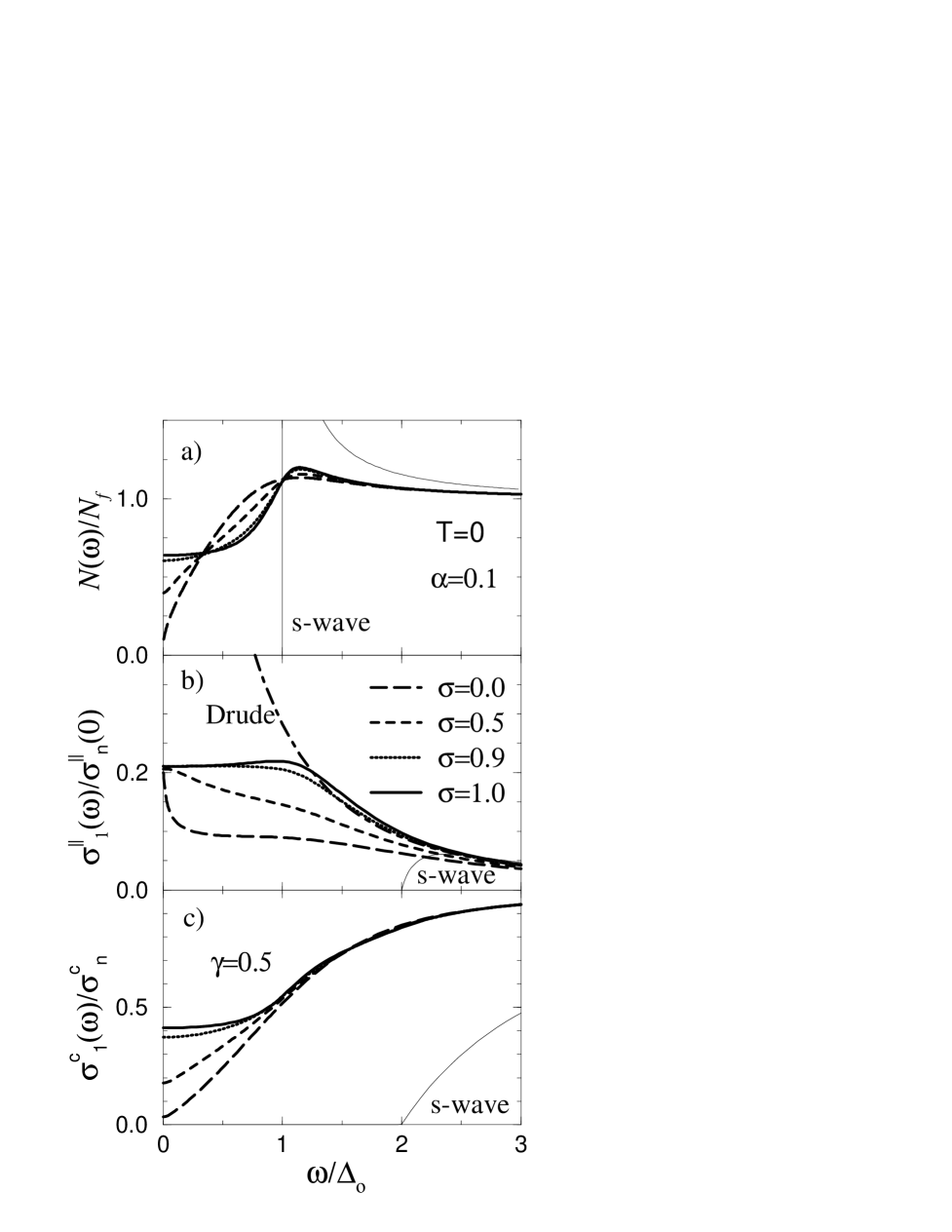
FIG. 3.: The density of states and the real part of the in-plane and $c$-axis conductivities at $T=0$, for a scattering rate described by $\alpha=\hbar/2\pi\tau\Delta_{0}=0.1$, and several values of the normalized scattering cross section $\bar{\sigma}$, as a function of frequency. All results are for a $d$-wave pairing interaction unless otherwise noted. (a) Density of states normalized by the density of states at the Fermi level. (b) The in-plane conductivity normalized by the normal state Drude value at $\omega=0$. (c) The $c$-axis conductivity normalized by the normal state value.

FIG. 4.: The temperature dependence of the in-plane and $c$-axis conductivities for a scattering rate of $\alpha=\hbar/2\pi\tau\Delta_{0}=0.01$, in the unitarity limit, as a function of frequency. a) The in-plane conductivity normalized by the normal-state Drude conductivity. b) The $c$-axis conductivity normalized by the normal-state value.

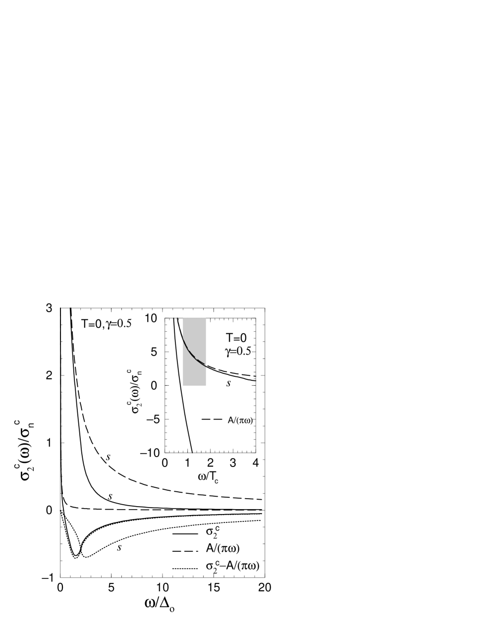
FIG. 5.: The imaginary part of the $c$-axis conductivity (reactance) at $T=0$ for a scattering rate described by $\alpha=\hbar/2\pi\tau\Delta_{0}\to 0$. The $s$-wave results are denoted by an $S$. We show $\sigma_{2}^{c}(\omega)=\mbox{Im\,}{\sigma^{\bot}(\omega)}$, and separately the London term, $A/\pi\omega$, and the difference of these two. The constant $A$ was extracted from $\sigma^{\bot}(\omega)$ by a Kramers-Kronig transformation. Inset: The $d$-wave result has been rescaled to yield the same penetration depth, $\lambda_{\bot}(0)$, as for the $s$-wave result (see text). The shaded region indicates the range of measured plasma frequencies, $\omega_{pc}$, in cuprate superconductors.

REFERENCES

- [1] Present address: Department of Physics and Astronomy, Northwestern University, Evanston, IL 60208, USA
- [2] D. Wollman et al., Phys. Rev. Lett. 71, 2134 (1993).
- [3] C. Tsuei et al., Phys. Rev. Lett. 73, 593 (1994).
- [4] D. Wollman et al., Phys. Rev. Lett. 74, 797 (1995).
- [5] D. Brawner and H. Ott, Phys. Rev. B 50, 6530 (1994).
- [6] A. Sun, D. Gajewski, M. Maple, and R. Dynes, Phys. Rev. Lett. 72, 2267 (1994).
- [7] M. Graf, D. Rainer, and J. Sauls, Phys. Rev. B 47, 12089 (1993).
- [8] L. Bulaevskiĭ, Zh. Eksp. Teor. Fiz. 64, 2241 (1973); [Sov. Phys. JETP 37, 1133 (1973)].
- [9] E. Kats, Zh. Eksp. Teor. Fiz. 56, 1675 (1969); [Sov. Phys. JETP 29, 897 (1969)].
- [10] M. Frick and T. Schneider, Z. Phys. B 78, 159 (1990).
- [11] S. Liu and R. Klemm, Phys. Rev. B 45, 415 (1992).
- [12] Y. Tanaka, Physica C 219, 213 (1993).
- [13] K. Sugihara, Phys. Rev. B 29, 5872 (1985); S. Shimamura, Synth. Met. 12, 365 (1985).
- [14] L. Ioffe, A. Larkin, A. Varlamov, and L. Yu, Phys. Rev. B 47, 8936 (1993).
- [15] J. Halbritter, Phys. Rev. B 46, 14861 (1992).
- [16] A. Koshelev, Zh. Eksp. Teor. Fiz. 95, 662 (1989), [Sov. Phys. JETP 68, 373 (1989).
- [17] N. Kumar, P. Lee, and B. Shapiro, Physica A 168, 447 (1990).
- [18] N. Kumar and A. Jayannavar, Phys. Rev. B 45, 5001 (1992).
- [19] A. Rojo and K. Levin, Phys. Rev. B 48, 16861 (1993).
- [20] R. Radtke, C. Lau, and K. Levin (unpublished).
- [21] A. Varlamov, Europhys. Lett. 28, 347 (1994).
- [22] S. Chakravarty, A. Sudbø, P. Anderson, and S. Strong, Science 261, 337 (1993).
- [23] R. Kleiner, F. Steinmeyer, G. Kunkel, and P. Müller, Phys. Rev. Lett. 68, 2394 (1992).
- [24] R. Kleiner and P. Müller, Phys. Rev. B 49, 1327 (1994).
- [25] K. Kadowaki and T. Mochiku, Physica B 194-196, 2239 (1994).
- [26] P. Müller, Advances in Solid State Physics (Vieweg, Braunschweig, 1994), Vol. 34.
- [27] R. Klemm, K. Scharnberg, D. Walker, and C. Rieck, Z. Phys. B 72, 139 (1988).
- [28] P. Hirschfeld et al., Phys. Rev. B 40, 6695 (1989).
- [29] P. Hirschfeld, W. Putikka, and D. Scalapino, Phys. Rev. B 50, 10250 (1994).
- [30] D. Pines, Physica C 235-240, 113 (1994).
- [31] G. Eilenberger, Z. Phys. 214, 195 (1968).
- [32] A. Larkin and Y. Ovchinnikov, Zh. Eksp. Teor. Fiz. 55, 2262 (1968), ; [Sov. Phys. JETP 28, 1200 (1969)].
- [33] G. Eliashberg, Zh. Eksp. Teor. Fiz. 61, 1254 (1971); [Sov. Phys. JETP 34, 668 (1972)].
- [34] J. Serene and D. Rainer, Phys. Rep. 4, 221 (1983).
- [35] J. Rammer and H. Smith, Rev. Mod. Phys. 58, 323 (1986).
- [36] A. Larkin and Y. Ovchinnikov, in Nonequilibrium Superconductivity, edited by D. Langenberg and A. Larkin (Elsevier Science Publishers, Holland, 1986), p. 493.
- [37] D. Rainer and J. Sauls, in “Strong Coupling Theory Of Superconductivity” (Spring College in Condensed Matter on “Superconductivity”, I.C.T.P. Trieste, 1992).
- [38] P. Muzikar, D. Rainer, and J. Sauls, in “The Vortex State”, edited by N. Bontemps, Y. Bruynseraede, G. Deutscher, A. Kapitulnik, NATO ASI series, (Kluwer Academic Publishers, Dordrecht, 1994) p. 244.
- [39] L. Keldysh, Zh. Eksp. Teor. Fiz. 47, 1515 (1964); [Sov. Phys. JETP 20, 1018 (1965)].
- [40] L. Buchholtz and G. Zwicknagl, Phys. Rev. B 23, 5788 (1981).
- [41] M. Graf, M. Palumbo, D. Rainer, and J. Sauls, Physica C 235-240, 3271 (1994).
- [42] Y. Tanaka, Phys. Rev. Lett. 72, 3871 (1994).
- [43] M. Sigrist and K. Ueda, Rev. Mod. Phys. 63, 239 (1991).
- [44] S. Yip and J. Sauls, J. Low Temp. Phys. 86, 257 (1992).
- [45] A. Abrikosov, L. Gor’kov, and I. Dzyaloshinski, “Methods of Quantum Field Theory in Statistical Physics” (Prentice-Hall, Englewood Cliffs NJ, 1963).
- [46] P. Müller, private communication.
- [47] V. Ambegaokar and A. Baratoff, Phys. Rev. Lett. 10, 486 (1963); 11, 104(E) (1963).
- [48] J. Halbritter, Phys. Rev. B 48, 9735 (1993).
- [49] S. Schmitt-Rink, K. Miyake, and C. Varma, Phys. Rev. Lett. 57, 2575 (1986).
- [50] P. Hirschfeld, D. Vollhardt, and P. Wölfle, Solid State Commun. 59, 111 (1986).
- [51] G. Preosti, H. Kim, and P. Muzikar, Phys. Rev. B 50, 1259 (1994).
- [52] C. Choi, Phys. Rev. B 50, 3491 (1994).
- [53] P. Lee, Phys. Rev. Lett. 71, 1887 (1993).
- [54] P. Wölfle, J. Low Temp. Phys. 95, 191 (1994).
- [55] K. Tamasaku, Y. Nakamura, and S. Uchida, Phys. Rev. Lett. 69, 1455 (1989).
- [56] C. Homes et al., Phys. Rev. Lett. 71, 1645 (1993).
- [57] J. Münzel et al., Physica C 235-240, 1087 (1994).
- [58] J. Kim et al., Physica C 247, 297 (1995).
- [59] M. Graf and M. Palumbo, J. Low Temp. Phys. 99, 283 (1995).
- [60] K. Zhang et al., Appl. Phys. Lett. 62, 3019 (1993).