How (Super) Rough is the Glassy Phase of a Crystalline Surface with a Disordered Substrate?

Abstract

We discuss the behavior of a crystalline surface with a disordered substrate. We focus on the possible existence of a super-rough glassy phase, with height-height correlation functions which vary as the square logarithm of the distance. With numerical simulations we establish the presence of such a behavior, that does not seem to be connected to finite size effects. We comment on the variational approach, and suggest that a more general extension of the method could be needed to explain fully the behavior of the model.

cond-mat/9503074

1 Introduction

Recently the two letters [1, 2](and a related comment, [2]) have stressed, by obtaining new numerical results, the interest of a problem that can be described in the first instance as the one of the surface of a crystal deposited on a disordered substrate.

The model has at today a long story. Renormalization Group ideas have been applied at first [3, 4, 5], while more recently the Mézard and Parisi [6] variational approximation has lead to the drawing of a quite different picture [7, 8, 9].

The relevant universality class describes indeed many and different physical situations. The first one, that we have already quoted, is the model of a crystal deposited on a disordered substrate. A second one is a two dimensional array of flux lines with the magnetic field parallel to the superconducting plane in presence of random pinning. Close to the phase transition (whose existence is predicted by the Renormalization Group and the by Variational Theory) the two models are expected to have the same critical behavior. The universality class is the one of the $2D$ Sine-Gordon model with random phases.

Let us define our system. The dynamical variables of the model are the integral displacements $d(x,y)$ of the surface from a disordered bidimensional substrate. The variables $x$ and $y$ take integral values going from $1$ to $L$. The number of points of the lattice is $S=L^{2}$. The displacements $d(x,y)$ take positive, negative or zero integral values. The disordered substrate is characterized by quenched random heights $\rho(x,y)$ in the range $(-\frac{a}{2},+\frac{a}{2})$, where $a$ is the elementary step of the surface columns (and will be one in the numerical simulations). The total height of the surface on the elementary $(x,y)$ square is

$$h(x,y)\equiv\ a\ d(x,y)+\rho(x,y)\ .$$ (1)

The Hamiltonian of the system is

$$H\equiv\frac{\kappa}{2}\sum_{x,y=0}^{L}\Bigl{[}\bigl{(}h(x,y)-h(x+1,y)\bigr{)}^{2}+\bigl{(}h(x,y)-h(x,y+1)\bigr{)}^{2}\Bigr{]}\ ,$$ (2)

where in the numerical simulations we will put the surface tension $\kappa$ equal to two. The partition function will be defined as

$$Z_{\rho}\equiv\sum_{\{d(x,y)\}}e^{-\beta H}\ .$$ (3)

We will consider a quenched substrate, i.e. the free energy $F$ will be defined as

$$F\equiv-\overline{\log Z_{\rho}}\ .$$ (4)

We will discuss here mainly about the height-height correlation function, which we define as

$$C(d)=\langle\bigl{(}h(\vec{r}_{0}+\vec{d})-h(\vec{r}_{0})\bigr{)}^{2}\rangle\ ,$$ (5)

where we only take the $2$ dimensional vector $\vec{d}$ of the form $(d,0)$ or $(0,d)$, and by $\langle\cdot\rangle$ we denote collectively the average over the different realizations of the noise, over the different origins and the thermal average.

In the Gaussian model with integral variables and no disorder, the surface is rough for $T>T_{R}$ [10]. In the warm phase the $C(d)$ of eq. (5) behaves as $\log(d)$. When $T<T_{R}$ the surface becomes flat, glued to the ordered bulk.

When one considers the case of a disordered substrate the situation is far less easy to analyze. The traditional approach to the problem is the one based on Renormalization Group ideas, while only recently the variational approximation approach by Mézard and Parisi [6] has been applied to the problem. The results one obtains in the two approaches have something in common. Both approaches find that there is a transition at $T=T_{R}=\frac{\kappa}{\pi}$. In the high $T$ phase thermal fluctuations make the quenched disorder irrelevant, and the systems behaves as the pure model. Here correlations behave logarithmically, i.e.

$$C_{T>T_{R}}(d)\simeq\frac{T}{\kappa\pi}\log(d)\ .$$ (6)

The differences come for $T<T_{R}$. In the Renormalization Group approach [3, 4, 5] one gets a new $\log^{2}d$ dominant contribution. Here one finds that

$$C^{(RG)}_{T<T_{R}}(d)\simeq a_{1}\log(d)+a_{2}\log^{2}d\ ,$$ (7)

where $a_{1}$ is non-universal, and $a_{2}$ is

$$a_{2}\equiv\Bigl{(}\frac{T_{R}-T}{T_{R}}\Bigr{)}^{2}\frac{2}{\pi^{2}}\ .$$ (8)

The presence of such a super-rough phase (where by super-rough we imply a $\log^{2}d$ behavior of the height-height correlation functions) is indeed an interesting potential implication of the presence of quenched disorder. Such a behavior would imply that the low $T$ phase is rougher than the high $T$ phase, that is quite unusual. At high $T$ thermal fluctuations are able to carry the surface away from the deep (but not deep enough) potential wells due to the quenched disorder. So the roughening is the same than for the pure model. At low $T$ the surface gets glued to the bulk. In the ordered case this makes the surface smooth, since the bulk is ordered. But in presence of the quenched disordered substrate this effect does not smooth the surface, but on the contrary forces it to follow a very rough potential landscape. This mechanism could force a super-rough behavior.

The application of the variational approximation [6] to this system [7, 8, 9] does not lead to presence of a $\log^{2}d$ term, but to a behavior similar to the one of the high $T$ phase, with a slope of the logarithmic term which freezes at the critical point

$$C^{(VAR)}_{T<T_{R}}(d)\simeq\frac{T_{R}}{\kappa\pi}\log(d)\ .$$ (9)

We will try to argue in section (3) that in some sense this is an intrinsic limit of a too straightforward application of the variational approximation (originally discussed for systems with continuous replica symmetry breaking [6]) to systems with a single step broken replica symmetry, and we will suggest that a more complex approach could be needed in order to get a fair picture of this kind of systems.

A numerical analysis of references [2, 1] was making indeed the mystery even greater. Systems which should belong to the same universality class seem to show a very different behavior. Reference [2] was unable to detect any signature of the glass transition when measuring static quantities in a continuum random phase model, that, as we said, should belong to the same universality class of our discrete model (but see the comment [2]). The authors of [1] study the model we have defined before, and seem to detect numerically a picture compatible with the variational ansatz. The approach suggested from Cule and Shapir seemed to us interesting, and worse to be pursued further. It has motivated us to run further simulations and more analysis of the numerical data, and to look better in the theoretical problem of selecting the correct analytic approach.

2 The Numerical Simulations

We have ran our numerical simulations on the APE parallel computer [11]. Our code, all written in a high level language and very elementary, was running at the $20\%$ of the theoretical maximal speed. The clear limit was the memory to the floating point unit bandwidth, that in our way to write the problem was limiting us to the $25\%$ of the theoretical efficiency. It would be surely possible and not very difficult to rewrite the code to obtain with an efficiency close to $50\%$. Our code was running at a sustained performance close to one Gflops on a APE tube (with a theoretical optimal performance close to the $5$ Gflops).

Our program was truly parallel, in the sense each lattice was divided among many processors. For example on a APE tube, which has $128$ processors arranged in a $3$ dimensional tubular shape of $2\times 2\times 32$ we were running a single lattice on $4$ processors, and we were running in parallel $32$ different random substrates in the third processor direction. With this approach the smaller lattice we could simulate is $4\times 4$. Our actual runs have all been using $L=64$ and $L=128$, simulating $256$ different substrate realizations and by evolving two uncoupled replica’s of the system in each random substrate (with a total of $512$ systems). The average over the disorder was taken over such $256$ realizations of the random quenched substrate.

We have started from a high value of $T$, running simulations for decreasing $T$ values. For $L=128$ we have used temperatures of 0.9, 0.8, 0.7, 0.65, 0.6, 0.45 and 0.35, while for $L=64$ we have used the values 1.0, 0.95, 0.9, 0.85, 0.8, 0.75, 0.7, 0.65, 0.6, 0.55, 0.50, 0.45, 0.40, 0.35, 0.30. At each $T$ value our run was starting from the last configuration of the higher $T$ value. We have been very conservative in requesting a long thermalization. At each $T$ value we have added for $L=64$ $.5$ millions full Monte Carlo sweeps of the lattice ($.7$ millions for $L=128$), and then we have measured the correlation functions $100$ times during $100,000$ further lattice sweeps. That turned out to guarantee a good statistical determination of the correlation functions. To check that in better detail we have chosen two $T$ values, one in the warm phase and one in the cold phase, i.e. $T=.60$ and $T=.35$ for $L=64$. On this lattice, starting from the final configurations, we have added first a series of $100,000$ more lattice sweeps, and measured expectation values again. Then we have repeated the procedure (all the measurements and the statistical analysis) by doubling the added run (i.e. with $200,000$ added sweeps), and by doubling it again (with $400,000$ added sweeps), and again (with $800,000$ added sweeps). For both $T$ values all results were compatible, and no transient effects were detected. The data points for the $L=128$ are always very similar to the ones on the smaller lattice, in all our range of temperatures. The dynamics was a simple Metropolis Monte Carlo simulation.

Let us note that all our numerical data are fully compatible (even if based on larger lattices and a better statistics), as far as we have been able to check, with the data of reference [1]. What differs here is the analysis of the data, and the fact that a more extensive data sample allows us to look in better detail to the relevant quantities. We will detect here a small effect, and the high statistics we have is crucial to be sure it is significant. We stress the importance of comparing the full set of correlation functions, at all distances, with the lattice form computed on the same value of the lattice size $L$. We also believe it is important to use the discrete form both for picking up the logarithmic behavior and for picking up the super-rough behavior which is dominated by a squared logarithm.

The lattice Gaussian propagator, which reproduces in the continuum limit the logarithmic behavior, is

$$P_{L}(d)\equiv\frac{1}{2L^{2}}\sum_{n_{1}=1}^{L-1}\sum_{n_{2}=0}^{L-1}\frac{1-\cos(\frac{2\pi dn_{1}}{L})}{2-\cos(\frac{2\pi n_{1}}{L})-\cos(\frac{2\pi n_{2}}{L})}\ .$$ (10)

As we have already stressed we also need a lattice transcription of the squared logarithmic term. It is natural to take

$$P_{L}^{(2)}(d)\equiv P_{L}(d)^{2}\ .$$ (11)

These are indeed the terms we have used to fit our numerical data and to try to distinguish a logarithmic behavior from a different asymptotic law.

In the following we will be comparing two possible behaviors of the correlation function $C(d)$. One is the Gaussian scaling

$$C(d)=a_{0}+a_{1}P_{L}(d)\ ,$$ (12)

while the second includes a quadratic term, i.e.

$$C(d)=a_{0}+a_{1}P_{L}(d)+a_{2}P_{L}^{(2)}\ .$$ (13)

In the case of an high temperature $T$, in the high $T$ phase, the Gaussian fit to the correct lattice propagator is very successful, and the non-Gaussian best fit gives a non-linear contribution compatible with zero. In this region we do not encounter any problem.

We will discuss in the following the low $T$ region, and we will use as an example the temperature $T=0.45$. In fig. (1) we plot the measured correlation function $C(d)$ versus the lattice Gaussian propagator, at $T=0.45$ on a lattice of size $L=128$. A linear fit looks at this level quite satisfactory. The discrepancy at low distances is not necessarily worrying, since we expect short distance modifications to the asymptotic behavior. We note for future comparison that the best fit gives here

$$C^{(all\ points)}_{(linear)}(d)=-0.02+0.62P_{L}(d)\ ,$$ (14)

by using here all data points in the fit. Let us note now that in this fit and in all the following but for the quadratic one, eq. (17), the errors (which we have estimated by a jack-knife approach) are very small, of the order or smaller than one percent. All the best fits have been found be exact minimization of the $\chi^{2}$ function, since in all cases it is quadratic in the parameters. The estimated linear coefficient is exactly the one one finds in the variational approach (since the lattice propagator is equal, in the continuum limit, to $(\mbox{const}\ +\ \frac{1}{2\pi}\log(r))$). A quadratic fit works here very well, but since it has one more parameter than the linear fit let us ignore this fact for a moment. The quadratic fit of eq. (17), with $3$ free parameters and done discarding $10$ distance points, has on the contrary a very large error, but we report it for the indications it gives about the reliability of the value we quote for the quadratic coefficient (see the following discussion). Fitting including distance points starting for example from $d=4$ would give a accurate determination of all parameters.

As a next step we plot in fig. (2) $C(d)$ divided by the lattice propagator $P_{L}(d)$ as a function of $P_{L}(d)$. Linearity of this quantity as a function of $P_{L}(d)$ implies the presence of a $\log^{2}$ term in the $C(d)$. The effect is very clear, and the evidence for the presence of such a contribution unambiguous. We find here that

$$\Bigl{(}\frac{C(d)}{P_{L}(d)}\Bigr{)}^{(all\ points)}_{(linear)}=0.52+0.12P_{L}(d)\ ,$$ (15)

again by using data points from all distances.

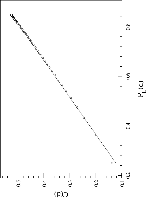
Figure 1: The measured correlation function $C(d)$ versus the lattice Gaussian propagator, at $T=0.45$ on a lattice of size $L=128$. The straight line is our best fit to a linear behavior, by using all distance data points.

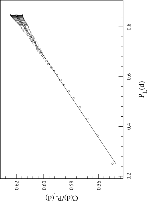
Figure 2: The measured correlation function $C(d)$ divided by the lattice Gaussian propagator versus the lattice Gaussian propagator, at $T=0.45$ on a lattice of size $L=128$. The straight line is our best fit to a linear behavior, by using all distance data points.

The only concern we are left with is that in the previous analysis we have used all distance points, while we are trying to resolve a long distance behavior. We have to be careful not to be mislead by short distance artifacts, which could obscure the true long distance behavior. In order to play safe, we plot in fig. (3) both $C(d)$ and $\frac{C(d)}{P_{L}(d)}$ as a function of $P_{L}(d)$ for distances larger than $10$ lattice units, and our best fits done by using only these distance points. In this case we fit $C(d)$ both to the linear and to the quadratic form. We get

$$C^{(d>10)}_{(linear)}(d)=-0.06+0.69P_{L}(d)\ ,$$ (16)

that is very similar to our previous fit, and

$$C^{(d>10)}_{(quadratic)}(d)=-0.014+0.56P_{L}(d)+0.093P_{L}^{(2)}(d)\ .$$ (17)

The most remarkable result is for the ratio we get

$$\Bigl{(}\frac{C(d)}{P_{L}(d)}\Bigr{)}^{(d>10)}_{(linear)}=(0.52\pm.01)+(0.12\pm.02)P_{L}(d)\ ,$$ (18)

with a very small $\chi^{2}$ and in complete agreement with what we got by fitting all data points. Two comments about two remarkable facts are in order. In first the linear coefficient of the best fit for the ratio is equal to the quadratic coefficient of the best fit for $C(d)$, and the constant coefficient in the ratio fit is equal to the linear coefficient of the quadratic fit to $C(d)$. In second discarding ten short distance points does not change the results for the linear and the quadratic contribution. We are definitely not looking at a short distance effect. Let us also notice that the reader could think that since the error on the different points of the divided $C(d)$ of fig. (3) are quite large the slope has to be compatible with zero. This is not true since the data points (different correlation functions for different $d$ values) are highly correlated, and the error over the slope has to be estimated directly. We have presented evidence that the value of the slope is non-zero.

Figure 3: The measured correlation function $C(d)$ and the measured correlation function divided by the lattice Gaussian propagator versus the lattice Gaussian propagator, at $T=0.45$ on a lattice of size $L=128$, after discarding the first ten distance points. The straight continuous lines are our best fits to a linear behavior, while the dotted line is the bets fit to a quadratic behavior of the function $C(d)$.

The fit to the form (13) gives a very good result both in the warm phase (where it coincides with the gaussian fit) and in the cold phase. The presence of a lattice term corresponding to a continuum $\log^{2}d$ behavior accounts very well for our numerical data. In fig. (4) we show the coefficients $a_{1}$ and $a_{2}$ from our best fits in all the temperature range we have explored (we use here all distance points). The continuous lines are only a visual aid, smoothly joining the numerical data points. The coefficient of the non-linear term $P_{L}^{(2)}$ becomes sizeably different from zero exactly close to the critical temperature $T_{c}=\frac{2}{\pi}$. The effect is quite clear and convincing. The coefficient $a_{1}$ is not the one of the $\log(d)$ term in the continuum limit, that is renormalized by a contribution coming from the $P_{L}^{(2)}(d)$ term. We find that the coefficient of the continuum $\log^{2}$ term is of the order of $5$ times smaller than the universal value we would expect from the RG computations. This is a fact that will have to be understood in better detail. The linear dependence of $a_{1}$ over $T$ in the high $T$ phase, where $a_{2}=0$, is very clear.

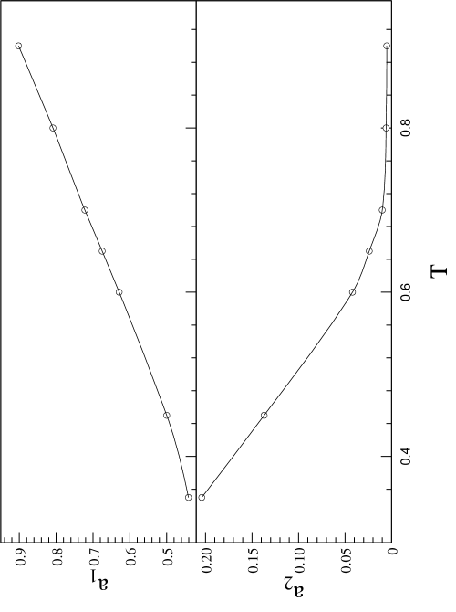
Figure 4: The coefficients $a_{1}$ and $a_{2}$ from our best fits to the form (13) versus the temperature $T$ in all the temperature range we have explored. Here $L=128$.

We believe that the previous evidence clearly shows that the ansatz of a purely gaussian probability distribution does not explain the behavior of the system for $T<T_{R}$, while the hypothesis of a super rough phase, with a $\log^{2}d$ behavior of the correlation functions, matches the numerical findings very well. In order to gather more information about this glassy phase we have looked at the probability distribution of

$$\Delta\equiv h-h^{\prime}\ ,$$ (19)

where $h^{\prime}$ is a first neighbor of $h$. In order to monitor the shape of the probability distribution we plot in fig. (5) the related Binder parameter defined as

$$B_{L}^{(\Delta)}(T)\equiv\frac{1}{2}\Bigl{(}3-\frac{\langle\Delta^{4}\rangle}{\langle\Delta^{2}\rangle^{2}}\Bigr{)}\ .$$ (20)

$B_{L}$ is zero for a gaussian distribution, and $1$ for a $\delta$-function. In our measurement it is very small in the warm phase, calling again for a very Gaussian behavior. On the contrary in the low $T$ phase we get a non trivial shape. Here $B_{L}$ is definitely non-zero, non-one, and in our $T$ range does not seem to depend on $L$. This shows again that in the cold phase there is a non-trivial behavior. A value of $B_{L}$ which is non trivial (non $0$ and non $1$) and does not depend on $L$ is reminiscent of a Kosterlitz-Thouless like situation. Further analysis will be required to reach a better understanding of the characteristic features of the low $T$ phase.

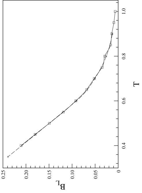
Figure 5: The Binder parameter $B_{L}^{(\Delta)}$ as a function of $T$ for the two values of the lattice size, $L=64$ and $L=128$.

3 Some Comments on the Variational Approach

We have already argued that the numerical results presented above do not coincide with the analytical predictions either of the Renormalization Group or of the Gaussian Variational approach. From the qualitative standpoint, the disagreement is even stronger with the latter since it predicts that the asymptotic correlation function grows only logarithmically with the distance. Consequently, one has a right to wonder how much the Gaussian Variational approach is trustworthy. Some general remarks on this issue will be given in this section.

As argued by Mézard and Parisi in their original paper [6], the Gaussian Variational Theory (GVT) is exact for the theory of an $N$-components field ${\vec{\phi}}({\bf x})$ in the limit $N\to\infty$ (while the model considered in this paper corresponds to $N=1$). This may be easily understood by noticing that the GVT coincides with the Hartree-Fock partial resummation of the graphs due to the interaction potential between the replicas [6]. If the quenched potential $V({\bf x},{\vec{\phi}})$ seen at point ${\bf x}$ by the field ${\vec{\phi}}$ is itself a Gaussian variable of zero mean and variance $\overline{V({\bf x},{\vec{\phi}})V({\bf x}^{\prime},{\vec{\phi}}^{\prime})}=\delta({\bf x}-{\bf x}^{\prime}){\cal R}({\vec{\phi}}-{\vec{\phi}}^{\prime})$ that is, with a purely local interaction, then the tadpole contribution to the self-energy $\sigma^{ab}(k)$ between two different replicas $a$ and $b$ will not depend upon the momentum $k$ and will only result in renormalization of the mass term. When the solution of the variational equations turns out to be consistent with a continuously replica broken mass term $\sigma(u)$ (where $0<u<1$ is the distance between the replicas), this is not a serious limitation and non trivial exponents may be found [6, 8, 9], related to the small $u$ behavior of $\sigma(u)$. On the contrary, when the solution consists of a finite number of breaking steps as in the present case, there is no such small $k$ - small $u$ cross-over, and the full propagator is proportional to the bare propagator at small $k$ (when $\sigma(0)=0$). This explains why the one-step Ansatz used in [8, 9] necessarily leads to a logarithmic growth of the correlation function which corresponds to the free behavior, the only non trivial prediction being the freezing of the coefficient of proportionality under $T_{R}$ (see formulae (6) and (9)).

An important example where the Gaussian Ansatz leads to erroneous results is the Random Field Ising Model (RFIM). Recently, Mézard and Young proposed a general method of adding momentum-dependent contributions to the self-energy $\sigma^{ab}(k)$ by considering a self-consistent expansion in $1/N$ of the variational free-energy [12]. Applying this method to the RFIM, they were able to show that the new graphs at $O(1/N)$ improved the Gaussian Ansatz and were sufficient to break the so-called dimensional reduction coming from usual perturbation theory, and which of course held at the Gaussian level. Such an approach could also be used to improve our theoretical understanding of the model studied in this paper. It suffers however from a mathematical difficulty related to the absence of solutions $\sigma^{ab}(k)$ with a finite number of steps of breaking, forcing one to look for a fully broken mass $\sigma(k,u)$. So far, no solution has been found in the case of the RFIM and one would probably have to face the same difficulties for the Random Sine-Gordon Model.

Beyond the quantitative calculation of the critical exponents, an important feature of the GVT is that it leads to a simple determination of the phase diagram of the model studied here. In this respect, the figures 4 and 5 seem to indicate that the distribution of the height differences $\Delta$ defined in (19) differs from a Gaussian even at temperatures higher than the usual theoretical prediction $T_{R}={\kappa\over\pi}$. As the two curves for the sizes $L=64$ and $L=128$ coincide quite well, finite size effects can apparently not account for this discrepancy. Some preliminary analytical results we have obtained using the GVT above $T_{R}$ hint indeed at a possible dynamical transition at a temperature $T_{d}$ ($T_{d}>T_{R}$) whose value depends on the amount of disorder given by the variance of the quenched displacement field $d(x,y)$ (see the introductive section). If this would be so, there would already exist at the temperature $T_{d}$ an exponentially large number (in $L^{2}$) of metastable states and the system would only partially “thermalize” in these traps. Both numerical and analytical work is currently in progress to investigate this important issue.

4 Conclusions

The results we have obtained describe a very complex picture. A super-rough behavior seems indeed to be there, implying that the GVT does not account fully for the behavior of the model. We are discussing here very small effects, so we cannot exclude completely that we are not looking at a transient behavior, but that does not seem likely at all. On the other side the coefficient of such a non-linear term seems to be, far out of statistical and systematic error, different from the one one obtains with a RG computation. Also, a non-trivial Binder parameter looks non-trivial even in the beginning of the to-be warm phase (that is maybe not the warm phase yet), suggesting the presence of a complex scenario also for temperatures $T$ of the order of $0.8$.

We have argued that indeed from the theoretical view-point we have some understanding of what is happening. We hope we will succeed to deepen it in the near future.

References

- [1] D. Cule and Y. Shapir, cond-mat/9411048, Phys. Rev. Lett. 74 (1995) 114.
- [2] G. G. Batrouni and T. Hwa, cond-mat/9403086, Phys. Rev. Lett. 72 (1994) 4133; H. Rieger, Comment on: Dynamic and Static Properties of the Randomly Pinned Flux Array, unpublished.
- [3] J. L. Cardy and S. Ostlund, Phys. Rev. B 25 (1982) 6899.
- [4] J. Toner and D. P. Di Vincenzo, Phys. Rev. B 41 (1990) 632.
- [5] Y.-C. Tsai and Y. Shapir, Phys. Rev. Lett. 69 (1992) 1773.
- [6] M. Mézard and G. Parisi, J. Phys. A: Math. Gen. 23 (1990) L1229; J. Physique I 1 (1991) 809.
- [7] J. Bouchaud, M. Mézard and J. Yedidia, Phys. Rev. Lett. 67 (1991) 3840; Phys. Rev. B 46 (1992) 14686.
- [8] T. Giammarchi and P. Le Doussal, Phys. Rev. Lett. 71 (1994) 1530; Elastic Theory of Flux Lattices in Presence of Weak Disorder, cond-mat 9501087 preprint (January 1995).
- [9] S. Korshunov, Phys. Rev. B 48 (1993) 3969.
- [10] S. T. Chui and J. D. Weeks, Phys. Rev. B 14 (1976) 4978; Phys. Rev. Lett. 40 (1978) 733.
- [11] See for example C. Battista, S. Cabasino, F. Marzano, P. S. Paolucci, J. Pech, F. Rapuano, R. Sarno, G. M. Todesco, M. Torelli, W. Tross, P. Vicini, N. Cabibbo, E. Marinari, G. Parisi, G. Salina, F. Del Prete, A. Lai, M. P. Lombardo and R. Tripiccione, The Ape-100 Computer: (I) the Architecture, International Journal of High Speed Computing 5 (1993) 637, and references therein.
- [12] M. Mézard and A.P. Young, Europhys. Lett. 18, 653 (1992).