Phason elasticity of a three-dimensional quasicrystal: transfer-matrix method

Abstract

We introduce a new transfer matrix method for calculating the thermodynamic properties of random-tiling models of quasicrystals in any number of dimensions, and describe how it may be used to calculate the phason elastic properties of these models, which are related to experimental measurables such as phason Debye-Waller factors, and diffuse scattering wings near Bragg peaks. We apply our method to the canonical-cell model of the icosahedral phase, making use of results from a previously-presented calculation in which the possible structures for this model under specific periodic boundary conditions were cataloged using a computational technique. We give results for the configurational entropy density and the two fundamental elastic constants for a range of system sizes. The method is general enough allow a similar calculation to be performed for any other random tiling model.

I Introduction

Quasicrystals are defined as structures which possess translational order to the extent that their Fourier transforms exhibit $\delta$-function Bragg peaks, but which have symmetries that are forbidden in a periodic Bravais lattice. A number of alloys have been found experimentally which appear to be true quasicrystals in this sense, such as i(AlCuFe) [1] and i(AlPdMn) [2, 3], which both exhibit resolution-limited Bragg peaks.

Two competing physical scenarios have been advanced to explain the origins of quasiperiodic ordering. One of them—the ‘ideal tiling’ scenario—postulates that the atomic structure of a well-annealed quasicrystalline sample is perfectly quasiperiodic, like the two-dimensional Penrose tiling [4] or its generalizations. In this scenario it is hypothesized that the microscopic Hamiltonian constrains the local arrangements of atoms in such a way as to implement something akin to Penrose’s local ‘matching rules’, which force long-range quasiperiodicity.

The alternative to this ideal tiling approach is the ‘random tiling’ scenario, which also makes use of local clusters of atoms, with packing rules similar qualitatively to Penrose’s rules but insufficiently strong to force a unique behavior at long distances. This gives rise to an ensemble of different ways of packing atoms into the space occupied by the sample. Normally we assume these different configurations to be nearly degenerate in energy. In the actual models studied, space is assumed to be filled by a finite set of local patterns which we represent by a set of tiles. Such models have a contribution to their entropy arising from the many ways in which the tiles may be packed. This entropy can reduce the free energy with respect to crystalline structures (which are expected to be stable at zero temperature), offering an alternative explanation of how the quasicrystal state might be stabilized [5, 6]. To date, random-tiling models have been studied in two dimensions with 8-fold [7, 8], 10-fold [5, 9, 10] and 12-fold symmetries [11], and in three dimensions with icosahedral symmetry [12, 13, 14].

In principle it should be possible to construct random-tiling models so that there is a one-to-one mapping of tiling configurations onto real atomic configurations, via deterministic rules that specify how the tiles are to be decorated with atoms. Then the configurational entropy (and other thermodynamic quantities) of the atomistic model will be identical to that of the tiling model. The decoration of random tilings to produce atomic models of the icosahedral phases is discussed in Refs. [15, 16, 17, 18].

This paper is principally concerned with random tiling models of quasicrystals. The qualitative predictions of these models and the ideal tiling models are very similar, to the extent that they are known. In particular both models predict the sharp Bragg peaks observed in experiments. Experiments aimed at resolving the differences between the two for real quasicrystals have still not conclusively settled the question one way or the other. However, there are some arguments we can present in favor of the random-tilings. One important point is that we have some understanding of how interatomic potentials might lead to a random-tiling structure. The simplest model for such a process is the 2D ‘binary tiling’, in which atoms of two different sizes aggregate in patterns which can be set in one-to-one correspondence with the configurations of a tiling of ‘fat’ and ‘skinny’ rhombi [9]. More recently, it has been shown in simulations that several 3D models with reasonable pair potentials for simple atoms (Al, Mg, Li, Zn) will freeze into structures which can be represented as configurations of a random tiling model [19, 58]. On the other hand, there is no understanding of how the thermodynamics of a system governed by a microscopic Hamiltonian might give rise to the matching rules necessary for the ideal tiling scenario. In fact, the most promising recent advance in this direction has been achieved at the expense of blurring the distinction between random tilings and ideal quasicrystal models: one assumes an ensemble in which any of a large number of tilings is permitted, but adopts a Hamiltonian such that the ground state, and the thermodynamic state if the temperature is not too large, is essentially an ideal quasicrystal [20].

A Phason elasticity

The long-wavelength behavior of random tiling models is described by a sort of Landau theory, which has two kinds of parameters: (i) the entropy density, and (ii) the ‘phason strain’ (see Sec. II). Most of the proposed experimental tests of the random-tiling scenario hinge around the expected variation of the entropy with this phason strain, which produces a kind of elastic term in the free energy. We describe this in more detail in the next section where we define the ‘phason elasticity tensor’, which measures the strength of this effect. It is predicted that the smallest eigenvalue of the phason elasticity tensor should decrease with decreasing temperature, producing instabilities of the quasicrystal phase with respect to other structures when the temperature becomes low enough [21, 22, 23].

Also, by contrast with the matching rule models, it is predicted that the phason elasticity for a random-tiling should have a gradient-squared form (see Section II A). This leads to diffuse ‘wings’ around peaks in the diffraction pattern, and to phason contributions to the Debye-Waller reduction of the Bragg intensities, both of which can in principle be measured experimentally to determine values for the elastic constants.

B Random canonical-cell tilings

In this paper, we build upon results from our previously published work [24], henceforth referred to as Paper I, to calculate a variety of properties of a random tiling ensemble based on the ‘canonical cell’ model of a quasicrystal. This model has been described in detail by Henley [25]. Briefly, it consists of vertices or ‘nodes’ which represent icosahedrally-symmetric clusters of atoms. Nearest-neighbor nodes are joined by ‘linkages’ of two types. Type $b$ linkages run parallel to the axes of two-fold symmetry of the reference icosahedron and are all of the same length which we denote $b$; type $c$ linkages run parallel to the axes of three-fold symmetry, and all have length $c\equiv b\sqrt{3}/2$. The linkages can form three kinds of polygon which in turn form the faces of four kinds of tiles or ‘canonical cells’ $A$, $B$, $C$, and $D$ into which the entire space is divided. (These cells were depicted in Fig. 1 of Paper I and also Fig. 1 of Ref. [25].)

In Paper I we gave an algorithm for generating a so-called ‘stacking graph’ for a random tiling, which we applied to the particular case of the canonical-cell tiling. This graph contains information about all possible structures that can be built out of a certain set of tiles with specified periodic boundary conditions. In this paper, we use this stacking graph as the basis for a transfer matrix calculation of the thermodynamic properties of the ensemble of random tilings of canonical cells, including the random tiling entropy and the phason elasticity [26]. These quantities have been found previously for another icosahedral random tiling, that of the two Ammann rhombohedra [14]. The canonical-cell model, however, is different in at least two respects:

• It lends itself to the construction of realistic atomic models for icosahedral quasicrystals such as i(AlCuLi) [16], i(AlMnSi) [18], i(TiCrSi) [17], and potentially i(AlPdMn). It is possible to construct decorations of the canonical cells which incorporate our understanding of the basic atomic motifs found in these alloys and which contain no points of unrealistically close or loose packing. Conversely it has not proved possible to relate the rhombohedron tiling to any good structure model.

• The canonical cell model is, unfortunately, much less tractable technically than the tiling of Ammann rhombohedra. In particular, Monte Carlo simulation has not been practicable because there is no known move that rearranges tiles locally and satisfies ergodicity. A possible chain-like or cluster move has been suggested by Oxborrow [15], but this move is still not completely understood. (It has been understood in a two-dimensional toy model, the square-triangle random tiling [11], which shares some features with the canonical-cell tiling.) Since we suspect that this kind of intractability is more generic than the behavior of rhombus and rhombohedron tilings [11, 27, 28], it behooves us to develop appropriate methods for studying less agreeable tilings such as the canonical-cell tiling, even if some other tiling ultimately proves more relevant to real quasicrystalline phases.

C Outline of the paper

The paper is organized as follows. In Section II we develop the elastic theory of random tiling ensembles, including the special cases that apply to the ensembles we will be studying with our transfer matrix method. In Section III we define our transfer matrix and explain how it is used to calculate thermodynamic properties of the ensemble as a function of phason strain. In Section IV we describe the calculations we have performed using the canonical-cell tiling, and give our results for the configurational entropy and phason elasticity of the tiling for a variety of system sizes. In Section V we present our conclusions.

II Phason elasticity in random tilings

In studying icosahedral tilings, it is convenient to use a basis of unit vectors ${\bf e}^{\parallel}_{\alpha}$ pointing from the center to vertices of the reference icosahedron, i.e., along the fivefold symmetry axes. It turns out that every type $b$ linkage can be written as the sum of four of these basis vectors and every type $c$ linkage can be written as the sum of three of them. Thus, having arbitrarily assigned ${\bf r}=0$ at one node, every other node in a canonical-cell tiling may be represented in the form

$${\bf r}=\sum_{\alpha=1}^{6}n_{\alpha}{\bf e}^{\parallel}_{\alpha},$$ (1)

where $n_{\alpha}$ are integers. The $\{{\bf e}^{\parallel}_{\alpha}\}$ are independent over integers so this representation is unique.

We can also define a ‘phason’ coordinate for each node

$${\bf r}^{\perp}=\sum_{\alpha=1}^{6}n_{\alpha}{\bf e}^{\perp}_{\alpha}.$$ (2)

The vector ${\bf r}^{\perp}$ lives in a space called ‘phason’ space or ‘perp’ space. As discussed elsewhere [21], with a proper choice of basis vectors $\{{\bf e}^{\perp}_{\alpha}\}$ the perp-space coordinate is well-defined. We can view Equations (1) and (2) together as defining a ‘lifting’ of the nodes to points on a six-dimensional hypercubic lattice; thus an arbitrary tiling configuration may be viewed as the projection of a three-dimensional surface embedded in six-space [29]. Following the conventions of Jarić [30], we write

$${{\bf e}^{\parallel}}_{1} = \eta(\tau,0,1),\qquad{{\bf e}^{\parallel}}_{2}=\eta(\tau,0,-1),\qquad{{\bf e}^{\parallel}}_{3}=\eta(1,\tau,0),$$ (3)

$${\bf e}^{\parallel}_{4} = \eta(0,1,\tau),\qquad{\bf e}^{\parallel}_{5}=\eta(0,-1,\tau),\qquad{\bf e}^{\parallel}_{6}=\eta(1,-\tau,0),$$ (4)

and

$${{\bf e}^{\perp}}_{1} = \eta(1,0,-\tau),\qquad{{\bf e}^{\perp}}_{2}=\eta(1,0,\tau),\qquad{{\bf e}^{\perp}}_{3}=\eta(-\tau,1,0),$$ (5)

$${{\bf e}^{\perp}}_{4} = \eta(0,-\tau,1),\qquad{{\bf e}^{\perp}}_{5}=\eta(0,\tau,1),\qquad{{\bf e}^{\perp}}_{6}=\eta(-\tau,-1,0),$$ (6)

where $\tau\equiv{1\over 2}(1+{\sqrt{5}})$ and $\eta\equiv(1+\tau^{2})^{-1/2}$ [31]. With these definitions, the length of the $b$-type linkage is $b=2\sqrt{1+2/\sqrt{5}}$. We also define a coarse-grained phason coordinate

$${\bf h}({\bf r})=\langle{\bf r}^{\perp}\rangle_{\bf r}$$ (7)

where $\langle\ldots\rangle_{\bf r}$ is an average over a neighborhood of ${\bf r}$. The phason strain tensor is then the gradient of ${\bf h}$ in real space:

$${\bf E}({\bf r})\equiv\nabla_{{\bf r}}{\bf h}({\bf r}).$$ (8)

A Form of the elasticity tensor

Consider an ensemble of tilings, possibly weighted with Boltzmann probabilities derived from some Hamiltonian ${\cal H}$. We hypothesize that the Hamiltonian is sufficiently small, or the temperature sufficiently high, that difference in energy between configurations is typically much less than $kT$, so that the free energy of the ensemble will be dominated by the entropy. We further make the assumption that the relative weighting of long-wavelength phason fluctuations (after coarse-graining) will be determined by a free energy of the form [32, 33]

$${\cal F}=\int_{V}d^{3}{\bf r}f({\bf E}({\bf r}))$$ (9)

where

$$f({\bf E})=f_{0}+{1\over 2}{\bf E}\cdot{\bf K}\cdot{\bf E}+{\rm O}({\bf E}^{3}).$$ (10)

${\bf K}$ is the elasticity tensor (really a 4-tensor) and $V$ is the system volume. In the case where the Hamiltonian ${\cal H}$ is zero for all states in the ensemble, $f_{0}$ is equal to minus the entropy per unit volume $S_{V}$ [34]. It is important to be aware that this form for the free energy is just a hypothesis. We cannot prove that $f({\bf E})$ must have an analytic minimum at ${\bf E}=0$, though it can be shown that, if the linkages in our tiling are uniformly distributed over all orientations equivalent by icosahedral symmetry, then ${\bf r}^{\perp}$ is approximately constant. In other words, the hypersurface formed by the tiling in six-dimensional space is approximately flat, having only small phason fluctuations at non-zero wavevectors. Thus the phason strain can be thought of as parametrizing the deviation from icosahedral symmetry, making it natural for $f$ to have a minimum at ${\bf E}=0$ if the free energy is dominated by the entropy of the ensemble. It would in theory be possible for $f$ to have a non-analytic minimum at ${\bf E}=0$. However, in all models previously studied the analytic form (10) as been borne out both by analytic calculations and by simulations [12, 13, 35]. Furthermore, a random tiling has long-range order (i.e., Bragg peaks exist) if and only if ${\bf h}({\bf r})$ has finite variance; this can be shown to follow from the gradient-squared form (10).

It is common to deal with (10) by assuming that the net phason strain is zero and then re-expressing (10) in terms of Fourier components ${\bf h}({\bf q})$ (this generalizes trivially to the case of any fixed background phason strain—see Section II B below). The result is a sum over wavevectors ${\bf q}$ of terms each of which is a quadratic form in the three components of ${\bf h}({\bf q})$. The coefficients are linear in $\{K_{i}\}$ and quadratic in the components of ${\bf q}$. This form is simpler than (10), since we write a quadratic form in three instead of nine quantities (and, what is more, the different ${\bf q}$ vectors decouple), and is appropriate for analyzing fluctuations from Monte Carlo simulations. However, the ensemble we will be working with in the present study permits undetermined phason strains with respect to only the (real space) $z$ direction, and we measure only the elasticities associated with that direction. In this case the Fourier analysis is not useful, and we must struggle with the full form of the elastic free energy.

The elastic free energy for icosahedral symmetry can be written [30, 36, 37]

$$f({\bf E}) = {1\over 2}K_{1}\sum_{ij}E_{ij}E_{ij}+{1\over 2}K_{2}\{(E_{11}+E_{22}+E_{33})^{2}-{4\over 3}\sum_{ij}E_{ij}E_{ij}+$$ (12)

$$(\tau E_{12}+\tau^{-1}E_{21})^{2}+\mbox{cyclic permutations}\}+{\rm O}({\bf E}^{3}).$$

If the icosahedral phase is to be stable against decomposition into other, possibly periodic phases, the quadratic stationary point in the free energy must be a minimum, rather than a saddle point or maximum. This requires that $K_{1}$ be positive definite, and $K_{2}$ may have either sign but must lie within the range

$$-\frac{3}{5}<K_{2}/K_{1}<\frac{3}{4}.$$ (13)

The values of $K_{1}$ and $K_{2}$ are one of the main points of contact between quasicrystal experiments and random-tiling theory. Knowing merely the ratio $K_{2}/K_{1}$ between the two is enough to determine the form of the diffuse scattering from the random tiling.

B Background phason strain

Consider now the case of a tiling with periodic boundary conditions in all three real space directions. The periodicity of the structure is represented by a set of vectors $\{{\bf a}_{i}\}$, which are the displacement in real space from a node to the corresponding node in another periodic repetition of the structure. Since the vectors ${\bf a}_{i}$ connect nodes, they can be written in the form (1), each with a corresponding perp displacement ${{\bf a}^{\perp}}_{i}$. The boundary conditions then constrain the system to have a global average phason strain ${\bf B}$, defined by the linear system of equations

$${\bf B}\cdot{\bf a}_{i}={{\bf a}^{\perp}}_{i}.$$ (14)

It will still be possible to consider fluctuations in the phason strain at finite wavevectors around this state, but when we consider the free energy associated with the phason elasticity, we must allow for the constraint on the long-wavelength phason strain by introducing Lagrange multipliers. We will not follow through the complete analysis here, but merely quote the important results, which are

• The elastic free energy density $f$ is shifted by a constant term $f_{0}={1\over 2}{\bf B}\cdot{\bf K}\cdot{\bf B}$.

• The quadratic term becomes ${1\over 2}({\bf E}-{\bf B})\cdot{\bf K}\cdot({\bf E}-{\bf B})$.

• Most significantly, cubic and higher anharmonic terms now give contributions to the new quadratic term. Thus the elasticity tensor in the presence of the background phason strain loses its icosahedral symmetry and retains only the symmetry of the Bravais lattice defined by the periodic boundary conditions. The deviations, however, will be at most of ${\rm O}({\bf B})$ (from the cubic terms). Such terms in the elasticity were first measured by Oxborrow [11].

C Elasticity theory for a tower

In most of this paper, we consider a ‘tower’ in which periodic boundary conditions are applied in only the $x$ and $y$ directions; in the $z$ direction the tower can be arbitrarily large. The towers we will be considering have a square base and, of the icosahedral symmetry operations, only $x$, $y$, and $z$ reflections will be symmetries of the ensemble of possible configurations of cells in the tower; in particular, notice that the $x$ and $y$ axes will be inequivalent, even though the dimensions of the base in the $x$ and $y$ directions are equal, since the icosahedral point group has no 4-fold axis of symmetry.

For such a tower, only gradients with respect to the real-space $z$ coordinate remain free. Gradients with respect to $x$ and $y$ are fixed by the periodic boundary conditions, giving rise to a background phason strain of the type discussed above. We define ${\bf B}$ for a tower just as before except that the components ${\bf B}_{\alpha 3}$ are zero. Then

$$B_{11}=B_{22}=B$$ (15)

with

$$B=\tau^{-(2n+3)},$$ (16)

where $n$ is the order of the approximant, with $n=1$ for the $\frac{2}{1}$ structures, $n=2$ for the $\frac{3}{2}$, and so forth. All other components of ${\bf B}$ are zero. For the phason strain tensor ${\bf E}$, the boundary conditions give us just three free components $E_{\alpha 3}$ out of the nine. These three components transform like a vector, which we will call ${\bf A}$, with

$$A_{\alpha}\equiv dh_{\alpha}/dz\equiv E_{\alpha 3}.$$ (17)

We can write the free energy density for the tower in terms of this vector as

$$f({\bf A})=f_{0}+\frac{1}{2}\left\{C_{1}A_{1}^{2}+C_{2}A_{2}^{2}+C_{3}(A_{3}-A_{3}^{(0)})^{2}\right\}.$$ (18)

There are no cross-terms, because of the reflection symmetry, but the linear term shown involving the constant $A_{3}^{(0)}$ is possible because the $z$ reflection symmetry reverses both $h_{3}$ and $z$.

Using Equation (12), we can show that the constants in this formula are given by

$$C_{1} = K_{1}+(\tau^{2}-\frac{4}{3})K_{2}$$ (19)

$$C_{2} = K_{1}+(\tau^{-2}-\frac{4}{3})K_{2}$$ (20)

$$C_{3} = K_{1}-\frac{1}{3}K_{2}$$ (21)

and

$$A_{3}^{(0)}=-2BK_{2}/(K_{1}-\frac{1}{3}K_{2}).$$ (22)

We will calculate values for $C_{1}$, $C_{2}$, $C_{3}$, and $A_{3}^{(0)}$ using a transfer matrix method. Since these quantities are all functions of two elastic constants $K_{1},K_{2}$, there is some redundancy in such a calculation, which allows us a check on the accuracy of our methods. Inaccuracies can be ascribed to either (i) finite-size effects or (ii) finite-$B$ effects (through the cubic terms in the elasticity theory, which we omitted).

D Frequencies of objects in tiling

The relative frequency with which various types of tiles appear in a random tiling is directly related to the phason strain. For example, in the case of certain extreme phason strains, the tiling can be composed entirely of one type of tile. In some random tilings, the number densities of the different tile types is fixed exactly by the phason strain. The two-dimensional Penrose tiling of rhombi is one such example. In the canonical cell tiling this is not the case, but there are still things we can say about the relationship of the number density of tiles to the phason strain. These topics were discussed in detail in Ref. [25]. Here, we will just summarize the situation.

In addition to the phason strain, we can define many other macroscopic variables as the density (per unit volume) of occurrences of selected local patterns in the tiling. There are two reasons why we are interested in such patterns:

• When we come to decorate our tilings with real atoms to create possible atomic structures for icosahedral alloys, the simplest choice we can make is to use a single decoration for each type of canonical cell. In some cases a more satisfactory structure can be produced using a “context-dependent” rule, in which the decoration of a tile depends on the those of the tiles surrounding it. In either case the decoration depends on the local patterns in the tiling and the density and stoichiometry of the resulting structure are simple functions of the densities of those patterns.

• As discussed below in Section III D, iteration of the transfer-matrix always generates an ensemble which maximizes the entropy per layer, whereas we actually want the ensemble which maximizes the entropy per unit volume. We will be introducing chemical potentials which couple to the densities of local patterns in the tiling. By varying these chemical potentials, we can vary the relative frequency in the tiling of the various patterns and so generate an ensemble which is closer to the desired one [38].

The simplest and most important of the density variables are the densities of the tiles $A$, $B$, $C$, and $D$. In fact, these densities can be parameterized by just one independent parameter $\zeta$, which is defined as the volume ratio $V(D)/[V(A)+V(D)]$, where $V(X)$ is the total volume occupied by tiles of type $X$. (This follows because $V(B)$ and $V(C)$ are unique functions of the phason strain—see Eqs. (3.1) and (3.6) of Ref. [25].) This is important not only because $\zeta$ determines the stoichiometry and density of simple decoration models, but also because it completely determines the density of nodes, i.e., the frequency of the cluster motif in those models. Furthermore, the bulky $D$ cell tends to force its surroundings, so increases in its density tend to decrease the entropy density and increase the volume added per dead-surface (see Sec. III A below). Thus, the chemical potential conjugate to $\zeta$ is the most important one for approaching the correct ensemble.

We can write a more general form for the free energy $f({\bf E};\zeta)$ which has an absolute maximum at ${\bf E}=0,\zeta=\zeta_{0}$. (Possibly it might depend on additional density parameters also, but for the moment we will stick to this simplest case.) Then the expansion of $f$ around this maximum will contain terms such as ${1\over 2}K_{\zeta}(\zeta-\zeta_{0})^{2}$, where $K_{\zeta}$ is a new elastic constant. (Cross terms between $\bf E$ and $\zeta$ are forbidden by symmetry.) In the present calculations, this extra elastic constant is not physically relevant, for reasons which we discuss in Section III D below, so we define the entropy as the maximum $S({\bf E})=\max_{\zeta}[S({\bf E},\zeta)]$, making it a function only of the phason strain.

III Transfer matrix approach

In the majority of previous calculations on three-dimensional random tilings, workers have made use of Monte Carlo methods to study the elastic properties. In two dimensions on the other hand, the transfer matrix method has probably been as important as Monte Carlo simulation [7, 39, 40, 41]. General views of the transfer matrix method as applied to two-dimensional quasicrystals may be found in Ref. [21], Sec. 8.5.1, and in Ref. [33]. Transfer matrices provide a potentially exact way to calculate phason elasticity, and are more convenient for calculating entropies, which can be extracted from a Monte Carlo simulation only after integrating an entropy differential from zero to infinite temperature [11, 14, 42]. In the case of the twelve-fold ‘square-triangle’ tiling [11], a transfer-matrix formulation has made possible an exact solution with analytic expressions for the entropy density and the elastic constants [41, 43].

In the case of the canonical cell tiling, the implementation of a Monte Carlo simulation has, as noted above, been blocked by the lack of an update move. So instead, we have applied the transfer matrix method, using a new technique, which we now describe.

As described in Section II C, we consider an ensemble of all configurations filling a ‘tower’ with a given, finite base and having periodic boundary conditions in the transverse ($x$ and $y$) directions, but unbounded in the $z$ direction. This reduces our three-dimensional problem to one which is essentially one-dimensional, and therefore amenable to a transfer matrix treatment. We specialize to the ‘maximally random’ ensemble of tilings [21], meaning that each tiling configuration has equal weight (the Hamiltonian ${\cal H}$ is zero).

In Paper I we demonstrated how our towers can be decomposed into layers, and how the set of all possible towers may be codified in a ‘stacking graph’, which represents all the different ways of stacking these layers one on top of another. In this section we review this development and then discuss how the stacking graph may be turned into a transfer matrix whose eigenvalues are related to the free energy of the ensemble of tilings. We will also have to deal with a few technicalities associated with the facts that (i) the layers do not have equal volume and (ii) we must be able to compute the free energy for any accessible phason strain.

A Dead-surfaces and the stacking graph

The basis of our transfer-matrix approach is a rule for representing any given tower of cells by a sequence of layers of cells stacked in the $z$ direction, with a one-to-one correspondence between possible tilings and sequences of layers. Given that we can formulate a rule for dividing our tower of cells into these layers (possible strategies for doing this are discussed below) we can then construct a ‘stacking graph’ for the complete ensemble of tilings. The stacking graph consists of vertices joined by arrows (see Fig. 4 of Paper I, for example) where each vertex represents one kind of layer, and an arrow from one vertex to another represents a possible way in which the first kind of layer can be followed by the second. Any possible structure can then be described by a particular path through the stacking graph.

There are two different approaches to dividing a system into layers. In the first approach, which has been used in all previous transfer matrix studies of random tilings, one slices the structure up into slabs of cells, which span the entire cross-section of the tower from side to side. The average number of cells in a slab thus scales with the cross-sectional area. In two dimensions, the layers can often be mapped onto rows of sites on some lattice. By interpreting the stacking direction as a ‘time’ axis, conditions on the allowed transitions from one layer to the next can then be interpreted as local rules for the hopping of a conserved set of particles moving in one dimension. Making use of this idea for the case of the square-triangle tiling, a Bethe ansatz solution has been found [41], yielding exact analytic values for the entropy and elastic constants [43].

The decomposition of three-dimensional tilings into slabs is much less promising since each layer is itself a 2D random tiling spanning the cross-section of the tower. At every step in the construction of the stacking graph, we would need to completely enumerate all the possibilities for the next layer, and the number of such possibilities would grow exponentially as a function of the cross-sectional area, making the stacking graph extremely convoluted. So in Paper I we introduced a different approach, in which towers of canonical cells are divided into layers separated from one another by ‘dead surfaces’ [44]. Using this method, we generated the stacking graph and applied it to the production of an exhaustive list of periodic structures on the square ‘$\frac{5}{3}$’ base [24].

The notion of a ‘dead surface’ is linked with that of ‘forcing’. Imagine that we build a tower of cells, starting from some initial base, by adding nodes one at a time to the open top surface. Often, the top surface will have certain crevices which force the addition of a node at a particular place. The reason for this is that there are a number of linkages leaving each vertex in the surface, and there are only a finite number of different ways in which linkages are allowed to meet at a vertex. It is possible therefore, and indeed quite common, for the linkages which are already in place to restrict the number of possible choices for the ways in which a vertex can be completed. Thus the addition of a linkage or linkages around that vertex may be ‘forced’, and with these forced linkages come new vertices that sit at their other ends. These are our forced nodes.

A surface which has no forced nodes around any of its vertices is called a ‘dead surface’. We can produce a dead surface by taking a tower of canonical cells and adding all forced nodes to the top until no more additions are forced. The only choices we have to make in the construction of the tower are the ones we make about which node to add next when we are at a dead surface. Thus, a list of the successive dead surfaces and the choices we made when we got to them are sufficient to specify the tiling uniquely. The typical number of cells between two successive dead surfaces is relatively small, and approaches a small limit as the cross-sectional area of the tower diverges, so that the work involved in finding a surface does not increase indefinitely with the size of the system. And, most important, the stacking graph is sparse, in the sense that there only a small number (usually two) of possible successors to a given dead surface (by contrast with the slabs approach, in which there are exponentially many as the area of the slabs becomes large) [45]. The ‘dead surface’ and ‘slab’ approaches are contrasted in Fig. 1, using the two-dimensional square-triangle tiling for pedagogical purposes.

B Construction of the transfer matrix

If we were simply to generate tilings at random by taking random paths through the stacking graph and reconstructing the towers of cells to which they correspond, we would not generate tilings with the same weights with which they appear in our ensemble. To see this, consider a stacking graph in which, say, layer 1 can lead to two different layers, numbered 2 or 3; taking a random sequence means we would go to layer 2 or 3 with equal probability. But in the random-tiling ensemble, it may be that layer 2 is more likely than layer 3. That will be the case if layer 2 ultimately leads to a larger number of tilings afterwards than layer 3 does. If we specify that all tilings should appear with equal weights (${\cal H}=0$), that is not the same as saying that all transitions from one layer to another appear with equal weights. It is in order to tackle this problem that we introduce the transfer matrix.

As explained in the preceding section, a tiling of $M$ layers is uniquely represented by a sequence of dead surfaces and the choices made to continue growing the tiling at each surface. We will denote this $(\sigma_{m},l_{m})$ with $m=1,\ldots,M$ where $\sigma_{m}$ is the label of the $m^{\rm th}$ dead surface and $l_{m}$ is the label of the transition $\sigma_{m}\to\sigma_{m+1}$ in the stacking graph. (Normally there will only be one choice we can make at surface $\sigma_{m}$ that will lead us to surface $\sigma_{m+1}$. But occasionally there will be more than one way to make the transition, and in these cases we use the label $l_{m}$ to distinguish between them.)

We also partition the Hamiltonian into terms which each involve just two surfaces and the tiles contained between them:

$${\cal H}=\sum_{m=1}^{M}U(\sigma_{m},\sigma_{m+1},l_{m}).$$ (23)

Then the partition function can be written as

$${\cal Z}=\sum_{\{\sigma_{m},l_{m}\}}{\rm e}^{-{\cal H}}=\mathop{\rm Tr}\nolimits{\bf T}^{M},$$ (24)

where ${\bf T}$ is the transfer matrix. The general form for the elements of the transfer matrix is

$$T_{\sigma\tau}\equiv\sum_{l}{\rm e}^{-U(\sigma,\tau,l)}.$$ (25)

Note that $T_{\sigma\tau}$ is zero if there is no connection $\sigma\to\tau$ in the stacking graph; for the particular case ${\cal H}=0$, $T_{\sigma\tau}$ is just the number of ways to get from $\sigma$ to $\tau$.

The total weight in the partition function of all configurations of $M$ layers starting with layer $\sigma$ and ending with layer $\tau$ is then $({\bf T}^{M})_{\sigma\tau}$. It can be seen that, whatever boundary conditions we choose for the first and last layers, the free energy per layer in the thermodynamic limit is

$$F_{layer}=-\ln\Lambda_{max}$$ (26)

where $\Lambda_{max}$ is the largest eigenvalue of ${\bf T}$.

We are interested in computing the free energy for a range of phason strains, and also for a range of values of the parameter $\zeta$ (see Section II D). This means we must consider (i) how to measure the mean phason strain and density of a given ensemble, and (ii) how to generate ensembles with differing phason strain and density. These are dealt with in the next two subsections.

C Expectations

Having found the dominant eigenstate of the transfer matrix, we can extract the expectation of any operator ${\cal Q}$ that can be written in the form of a sum over the transitions from one dead surface to the next:

$${\cal Q}=\sum_{m=1}^{M}Q(\sigma_{m},\sigma_{m+1},l_{m}).$$ (27)

If $v^{(L)}$ and $v^{(R)}$ are the left and right eigenvectors corresponding to $\Lambda_{max}$, then the expectation of ${\cal Q}$ is

$$\langle{\cal Q}\rangle=\sum_{\sigma,\tau,l}v^{(L)}_{\sigma}{\rm e}^{-U(\sigma,\tau,l)}Q(\sigma,\tau,l)v^{(R)}_{\tau}.$$ (28)

Thus, for example, the expectation of the Hamiltonian, which is just the average energy per layer of the random tiling is

$$\langle U\rangle=\sum_{\sigma,\tau,l}v^{(L)}_{\sigma}{\rm e}^{-U(\sigma,\tau,l)}U(\sigma,\tau,l)v^{(R)}_{\tau}.$$ (29)

A number of other useful operators besides the Hamiltonian may be written in the form (27). In particular, having designated a representative node on each dead surface, we can define vectors ${\bf R}(\sigma,\tau,l)$ and ${\bf H}(\sigma,\tau,l)$ which are respectively the step in physical space and in perp space from one dead surface to the next. Then the total offset in physical and perp space are given by

$${\bf R}_{tot}=\sum_{m=1}^{M}{\bf R}(\sigma_{m},\sigma_{m+1},l_{m})$$ (30)

and

$${\bf H}_{tot}=\sum_{m=1}^{M}{\bf H}(\sigma_{m},\sigma_{m+1},l_{m}).$$ (31)

In the thermodynamic limit, the phason strain tensor ${\bf E}$ is then given by

$${\bf H}_{tot}={\bf E}\cdot{\bf R}_{tot}.$$ (32)

Six of the nine components of ${\bf E}$ take fixed values which we already know (see Section II C). The remaining three we calculate from (32).

We can also write the total number of nodes as

$$N_{tot}=\sum_{m=1}^{M}N(\sigma_{m},\sigma_{m+1},l_{m}).$$ (33)

where $N(\sigma_{m},\sigma_{m+1},l_{m})$ is the number of nodes added between surfaces $m$ and $m+1$. Since the total volume is given by

$$V_{tot}=[{\bf R}_{tot}]_{z}a^{2}$$ (34)

(where $a$ is the length of the edge of the square base), the number density of nodes is given by the ratio $N_{tot}/V_{tot}$.

D Chemical potentials

We wish to investigate ensembles of towers of canonical cells with different mean phason strains, so as to be able to maximize the random tiling entropy as a function of phason strain. In order to vary the average values of the three free phason strain components in our ensemble, we need to introduce terms into our Hamiltonian which couple to the phason strain, as mentioned briefly in Section II D. For example, if we want a particularly large $E_{xz}$ component of phason strain, we should favor those transitions from one surface to another which contribute a large shift in the $x$ direction in perp space by comparison with the $z$ component of the accompanying real space shift. The appropriate form for the terms in the Hamiltonian to achieve this is $\kern-0.15pt\hbox{$\mu$}\kern-6.02548pt\kern 0.20004pt\hbox{$\mu$}\kern-6.02548pt\kern-0.15pt\raise 0.20004pt\hbox{$\mu$}\cdot{\bf A}$, where ${\bf A}$ is the vector introduced in Section II C composed of the three free strain components, and $\mu$$\mu$$\mu$ is a vector whose components are chemical potentials coupling to the phason strain. Then the entropy per layer $S_{layer}$ is given by Legendre transformation:

$$F_{layer}=-\ln\Lambda_{max}=-S_{layer}+\kern-0.15pt\hbox{$\mu$}\kern-6.02548pt\kern 0.20004pt\hbox{$\mu$}\kern-6.02548pt\kern-0.15pt\raise 0.20004pt\hbox{$\mu$}\cdot\overline{\bf A}$$ (35)

where $\overline{\bf A}$ is the mean phason strain. Physically, we are only interested in the case ${\cal H}=0$; the chemical potentials are added solely as auxiliary fields in order to probe the variation of the entropy with phason strain.

We can similarly introduce a chemical potential $\mu_{\zeta}$ coupling to the the parameter $\zeta$, or equivalently to the packing fraction of nodes. However, we assume that $\zeta$ is freely varying, since we do not envisage placing any physical constraint on our ensemble that would fix its value. So the appropriate course of action will always be to choose the value of $\mu_{\zeta}$ that maximizes the entropy density [46].

For a system which did have a non-zero Hamiltonian, the equilibrium value of the internal energy (where $T=1$) would be given by

$$U=S-\kern-0.15pt\hbox{$\mu$}\kern-6.02548pt\kern 0.20004pt\hbox{$\mu$}\kern-6.02548pt\kern-0.15pt\raise 0.20004pt\hbox{$\mu$}\cdot\overline{\bf A}-\mu_{\zeta}\zeta,$$ (36)

and the equilibrium free energy, which is also the free energy at which the entropy is a maximum, is given by the Legendre transform:

$$F=U-S+\kern-0.15pt\hbox{$\mu$}\kern-6.02548pt\kern 0.20004pt\hbox{$\mu$}\kern-6.02548pt\kern-0.15pt\raise 0.20004pt\hbox{$\mu$}\cdot\overline{\bf A}+\mu_{\zeta}\zeta=0.$$ (37)

So we can either look for the maximum of the entropy, or equivalently we can look for the zero of the free energy, to find the equilibrium values of ${\bf A}$ and $\zeta$. In our particular calculations we maximized the entropy.

It is not necessary, as it is in some models, that the maximum entropy occur at the point at which all the chemical potentials are zero. The zero of the chemical potentials in this model corresponds to the maximum of the entropy per layer, which has no particular physical significance. The physically interesting quantity in this case is the entropy per unit volume. This quantity is not trivially related to the entropy per layer, since different layers make different contributions to the volume of the system. The calculation actually performed involves finding the entropy per layer and then converting it to an entropy density by dividing by the mean volume per layer within the ensemble:

$$S_{V}={S_{layer}\over a^{2}\overline{R}_{z}},$$ (38)

where $\overline{R}_{z}$ is the $z$ component of the ensemble average of the operator ${\bf R}(\sigma,\tau,l)$. The mean volume per layer will vary with the chemical potentials as we weight layers of different volumes more or less heavily. Because of the reflection symmetry of the ensemble in the $x$ and $y$ axes, we do in fact expect the minimum entropy density to fall at $\mu_{x}=\mu_{y}=0$, but in general it will not also fall at $\mu_{z}=\mu_{\zeta}=0$ and so we must probe a range of values of these chemical potentials to find it, calculating the entropy density as shown above.

IV Results and discussion

Our calculation proceeds as follows. We define the transfer matrix ${\bf T}$ as in Equation (24) using the list of possible transitions from one dead surface to another for a particular system generated from the stacking graph of Paper I. The systems we have looked at are the square-base canonical cell tilings with base of length $\tau b$, $\tau^{2}b$, and $\tau^{3}b$ (known as the ‘$\frac{2}{1}$’, ‘$\frac{3}{2}$’, and ‘$\frac{5}{3}$’ sizes). Although the transfer matrix quickly becomes large as the system size increases (the $\frac{5}{3}$ system has a transfer matrix some 7000 elements on a side) it is very sparse, so that matrix multiplication can be performed quickly, in time of order the rank of the matrix rather than the number of elements. The great advantage of the method we have adopted is that the quantities we are interested can be calculated by evaluating only the largest eigenvalue of the matrix, and its associated left and right eigenvectors. We can find these by simply multiplying the matrix many times into a trial eigenvector. Assuming this trial eigenvector has a non-zero component in the direction of the lowest eigenstate of the matrix, this will quickly give us the lowest eigenstate, and either one of the left or right eigenvectors of the system. We then repeat the process to find the other eigenvector, and from these we can evaluate the free energy per layer of our ensemble from Equation (26) and the free phason strain components ${\bf A}$ from Equation (32) as well as the parameter $\zeta$. Using these we can evaluate the entropy density per node from Equation (38).

We then vary the values of the chemical potentials coupling to the phason strain and $\zeta$ to find the maximum of the entropy for the ensemble, and the quadratic variation about that maximum to extract the coefficients $C_{1}$, $C_{2}$, and $C_{3}$, and hence the phason elasticities. The most straightforward way to accomplish this turns out to be to repeat the calculation on a grid of values in the space of the three chemical potentials that make up the vector $\mu$$\mu$$\mu$, maximizing always with respect to the remaining potential $\mu_{\zeta}$, as discussed in Section III D. Then we perform a cubic least-squares fit to the resulting function. The quadratic terms in this fit give us our elasticities, and the cubic terms give us an estimate of the error involved in calculating second derivatives at the maximum using what is essentially a finite difference method.

For the ‘$\frac{2}{1}$’ system, which has a base of length $\tau b$ and a background phason strain of $\tau^{-5}$, we find that one of the horizontal components of the phason strain—the one that we call $A_{2}$—can only take one value no matter what sequence of layers we stack one on top of another. Thus the corresponding elasticity parameter, $C_{2}$, is infinite. The other two parameters are finite. For the ‘$\frac{3}{2}$’ system, which has a base of length $\tau^{2}b$ and a background phason strain of $\tau^{-7}$, all three $C$ parameters have finite values, but the system is still sufficiently constrained that the packing fraction of nodes, or equivalently the parameter $\zeta$, takes only one value independent of the order in which we stack surfaces to construct our tower, so that there is no possibility of allowing this parameter to fluctuate and maximizing the entropy with respect to it.

The first system large enough to exhibit the generic elastic behavior typical of towers of canonical cells with large bases is the ‘$\frac{5}{3}$’ system, which is also the largest system we have tackled. In this system, which has a square base of length $\tau^{3}b$ on each side and a background phason strain of $\tau^{-9}$, all three components of the strain vector ${\bf A}$ are free to fluctuate under the influence of their corresponding chemical potentials, as is the parameter $\zeta$ which measures the density of nodes of the tiling. Figure 2 shows a contour plot of the entropy surface $\max_{\zeta}[S({\bf A},\zeta)]$ as a function of the phason strains $A_{1}$ and $A_{3}$. The maximum entropy density is $6.00\times 10^{-3}$, and falls at $A_{1}=0$ and at a small non-zero value of $A_{3}$ ($=0.0077\ldots$), as predicted. (It also falls at $A_{2}=0$, though this is not evident from the figure.) We have also studied the dependence of the entropy on $\zeta$ and we find that for a given ${\bf E}$, it depends very sharply on $\zeta$. There is a narrow valley in the plot of $f({\bf E};\zeta)$ centered around the plane $\zeta=\zeta_{0}({\bf E})$. In consequence, if we fix $\zeta$, the apparent dependence of $f({\bf E})$ on ${\bf E}$ is very sharp. (Note that, for the 2/1 and 3/2 cases, $\zeta$ is in fact a function of $\bf E$—the values of the background phason strain are so high in those cases that the valley has zero width.)

If we just omit (set to zero) the $\mu_{\zeta}$ parameter, thereby accepting the ensemble which maximizes the entropy per layer at a given phason strain, then we find an entropy density which differs from the actual value by only about three parts in $10^{5}$. We assume that the difference produced by including terms in the Hamiltonian coupling to other densities of local tiling patterns is smaller still, and therefore that we were justified in neglecting them in this calculation.

The value of the parameter $\zeta$ at the maximum of the entropy for the $\frac{5}{3}$ ensemble was 0.334, which is close to the “magic” value of $\zeta=0.317$ obtained at the end of Ref. [25]. The corresponding packing fraction $\phi$ for spheres of radius $c$ placed on the nodes may be determined from formulas given in Sec. III A of Ref. [25]. After converting from the length units used there, we obtain

$$\phi={{\pi\sqrt{3}}\over{16}}\biggl{[}{4\over{\sqrt{5}}}\eta+2(1-\eta)(1-{\zeta\over 3})\biggr{]}.$$ (39)

where

$$\eta\equiv{1\over 2}(1-\tau^{9}\det{\bf E})$$ (40)

and $\det{\bf E}=B^{2}A^{(0)}_{3}$ in our case. For the $\frac{5}{3}$ ensemble, we find a value of $\phi=0.606$. Values for the other system sizes are given in the table.

The packing fraction at which the maximum entropy occurs can be written roughly as

$$\phi({\bf E})=0.6064-0.026(A_{3}-A_{3}^{(0)})$$ (41)

for the $\frac{5}{3}$ case, with virtually no dependence on $A_{1}$ or $A_{2}$. (It seems plausible that, with more general values of phason strain, it would depend on the determinant $\det{\bf E}$ of the strain tensor.) In other words, the optimal packing fraction is practically constant (varying $\sim 1$% over the range of possible phason strains.) In the $\frac{2}{1}$ and $\frac{3}{2}$ cases, $\phi$ is a unique function of the phason strain. In these systems the coefficient of variation with $A_{3}$ is respectively 3.5 and 0.5 times as large as in Eq. (41).

Values for the elastic parameters $C_{1}$, $C_{2}$, $C_{3}$, and for the phason strain at equilibrium $A_{3}^{(0)}$ for the various systems are given in Table I. The values do not fit the relations (21) very well, presumably because the system size is small. However, it is possible to make out some trends in the data as the system size increases:

• There is a clear tendency to oscillate between high and low values of the elastic constants from one approximant to the next.

• superimposed on this oscillation, there is also a strong tendency for $C_{m}$ to decrease with increasing system size.

The first of these trends is to be expected if the errors are caused by the large background phason strain $B$, in view of Equation (16). The same oscillation is seen in the Monte Carlo simulations of the rhombohedral tiling by Shaw et al. [13]. (See, for instance, Figure 2 in that paper.)

We suggest that (ii) is also a finite-$B$ effect. The phason strain tensor components define a 9-dimensional space, and there is a domain in this space (centered on zero) of allowed phason strains. The entropy density vanishes with singular derivatives at the boundary of this domain. When $B$ is large, the phason strain tensor is necessarily closer to the boundary of the allowed domain, and the second derivatives of the entropy density (including the coefficients $C_{m}$) are consequently larger. In addition, the tendency for $S_{V}$ to be larger for smaller systems also enhances $C_{m}$, because increasing the maximum value of a function, while at the same time decreasing the interval over which it must rise from 0 to its maximum and fall back to zero, obviously forces it to have a larger (negative) second derivative.

So what can we say about the extrapolation of the data to infinite system sizes? The entropy density $S_{V}$ at least, appears to be far from its asymptotic value in the systems we have studied here. Indeed, on the basis of these data alone, one could not really rule out $S_{V}=0$ in the infinite-system limit [47]!

For the coefficients $C_{m}$, in view of the large values of $C_{2}$ for the 2/1 and $C_{3}$ for the 3/2, we have extrapolated the inverses $C_{m}^{-1}$. We have assumed the behavior

$${1\over C_{m}^{(n)}}\approx{1\over C_{m}^{(\infty)}}+\lambda B,$$ (42)

where $C_{m}^{(n)}$ is the value of $C_{m}$ measured for the $n^{\rm th}$ approximant and $B$ is background phason strain. For each $C_{m}$, we have extrapolated from the pair $(2/1,5/3)$ and the pair $(3/2,5/3)$ and taken the mean of these as the extrapolated value, writing error bars to span the two independent extrapolations [48]. The results are given in the “extrap” column of the Table.

We have also performed a slightly different analysis of the $5/3$ system using just the 316 approximants described in Paper I. This calculation is detailed in Appendix A, and in the column marked “$\frac{5}{3}$ (F) in the table.

Each of these different estimates give us four quantities $C_{1}$, $C_{2}$, $C_{3}$, and $A_{3}^{(0)}$, but there are only two independent parameters $K_{1}$, $K_{2}$ to fit to them. This places constraints on the four quantities with which their measured values are not entirely consistent. However, we can certainly conclude that $K_{1}\approx 1$, and that $K_{2}$ is negative and fairly large (possibly close to the instability limit (13)). This sign of $K_{2}$ is opposite to that in the rhombohedral tiling, a fact that we can explain qualitatively by the following argument.

From (21) we have

$$K_{2}={C_{1}-C_{2}\over\tau^{2}-\tau^{-2}}$$ (43)

so that $K_{2}<0$ if and only if $h_{x}$ fluctuates more than $h_{y}$ as one walks along a path in the $z$ direction. Examining the tiling, we find that the linkages along such a path are dominated by the 2-fold $b$ linkage that runs entirely along $z$, and by the 3-fold $c$ linkage $(\pm\tau,0,\tau^{3})$. In our basis (6), these $c$ linkages have perp space components only in the $x$ directions, making the $x$-fluctuations large compared with the $y$ ones, which in turn makes $K_{2}$ negative. On the other hand, the linkage vectors in the rhombohedral tiling are just the basis vectors in (4); thus the dominant steps in the direction of the path are $\eta(0,\pm 1,\tau)$ which has fluctuations in the $h_{y}$ direction rather than the $h_{x}$ direction. Thus for that tiling $K_{2}>0$ [12, 13].

For applications of random tilings to structural fitting, the parameter of greatest interest is the effective phason Debye-Waller factor ${\bf B}^{\perp}$, which corresponds to the extra variance in perp space due to the randomness of the tiling. The experimental value of ${\bf B}^{\perp}$ is of the order of 1Ų. In Appendix B, using the ensemble of 316 packings [24], we find a crude theoretical estimate of ${\bf B}^{\perp}$ for the canonical-cell random tiling which is somewhat smaller.

Finally, we would like to consider whether there is the possibility of performing a calculation for a larger system. Probably there is. It would tax the power of the available computing resources, but it should be possible. We estimate (see Paper I) that the next largest size of system—the $\frac{8}{5}$ system—should have a stacking graph of about one million dead surfaces. Given that the average number of nodes added between one dead surface and another tends to a constant as the system becomes large, we expect the time taken to construct the graph to scale as the number of dead surfaces, and so we would require about 200 times as much CPU time to perform the calculation as we did for the $\frac{5}{3}$ system. With today’s high-performance computing resources, such a calculation would be just within the bounds of possibility.

V Conclusions

Using the results of a previously-presented method for breaking down and cataloging three-dimensional random tilings, we have defined a transfer matrix whose eigenstates describe the properties of an ensemble of random-tiling configurations in the shape of towers with a finite area base and infinite extent in the $z$ direction. The ensemble has a mean phason-strain and packing fraction controlled by chemical potentials whose values we can choose. The transfer matrix is sparse and so can be efficiently multiplied into a trial eigenvector to find the largest eigenvalue. This gives us the free energy density and thus the entropy density for the ensemble. Maximizing this with respect to the components of phason strain and the packing fraction we can find the equilibrium values of these quantities, and the variation of the entropy density about the maximum, which defines the phason elasticity constants which are related to experimentally measurable quantities such as phason Debye-Waller factors, and diffuse scattering close to Bragg peaks.

We have applied our method to the ‘canonical-cell tiling’ [25] for towers with a square base with sides taking the three smallest non-trivial lengths possible. For the two smaller of these systems, we find that the systems have additional constraints making their elastic behavior different from the generic behavior expected of large systems. The largest system we have studied, which we refer to as the ‘$\frac{5}{3}$’ system is the smallest one that exhibits the same elastic behavior as a large system. From this system we have extracted a value of $6.00\times 10^{-3}$ for the entropy per unit volume. The two fundamental elastic constants, $K_{1}$ and $K_{2}$, are over-determined by the transfer matrix calculation because elasticities corresponding to the strains in various directions are related by symmetries of the system. This gives us a way to estimate the (finite-size) errors in our calculation, and it turns out that the values for $K_{1}$ and $K_{2}$ are not very accurate for this smallest of systems. Our best estimate is that $K_{1}$ lies in the range 0.8 to 1.1, and $K_{2}<0$. In addition, the requirement that the tiling be elastically stable with respect to other phases means that $K_{2}/K_{1}>-\frac{3}{5}$.

It is interesting to compare our results for the canonical-cell tiling with those for the rhombohedral random tiling [12, 13]. In doing so, we must be careful to allow for the different lengths of the linkages making up these tilings.

In the rhombohedral tiling [14] the entropy per node $S_{N}$ is $\sim 0.24\pm 0.02$, whereas in the canonical-cell tiling [49] it is only $\sim 0.047\pm 0.01$. This is a result of the fact that the canonical-cell tiling is more constrained in the states it can take than the rhombohedral tiling. This constraint is also responsible for limiting the canonical-cell tiling to only 32 distinct local node environments [25]. By contrast, the node environments of the rhombohedral random tiling are chosen from $10\,527$ of different possibilities [50].

To compare the elastic constants of the two tilings, we first define a characteristic unit of phason strain $E_{0}$ to be the ratio of the perp- and real-space displacements of the fundamental linkage. $E_{0}$ is 1 and $\tau^{-3}$ for the rhombohedral and canonical-cell tilings, respectively. Then a dimensionless measure of the elastic constant $K_{1}$ is the corresponding decrease in free energy per node for a phason strain of magnitude $E_{0}$:

$$\Delta F_{N}=\frac{1}{2}K_{1}E_{0}^{2}/n,$$ (44)

where $n$ is the packing fraction of nodes. For the rhombohedral tiling, $n=0.6498$, $K_{1}=0.81\pm 0.01$ and $K_{2}=0.495\pm 0.02$, hence $\Delta F_{N}=0.263$; for the canonical-cell tiling, using the extrapolated values $\Delta F_{N}=0.28$, very similar to the rhombohedral case [51].

Although the results for the elastic properties of the small canonical-cell systems show signs of being strongly influenced by finite-size effects, we believe that it should be feasible using modern supercomputing resources to perform a similar calculation for a larger system which should yield a more accurate estimate of the elastic constants for the infinite random canonical-cell tiling. We also believe that the method we have presented, which is fundamentally different from transfer matrix methods previously used in the study of random tilings, should be applicable to any random-tiling model in any number of dimensions. Even if the canonical-cell model does not ultimately turn out to be as good a model of real icosahedral phases as some other (yet to be proposed) tiling, we believe this method will prove useful in the calculation of experimentally measurable properties of quasicrystals.

VI Acknowledgments

The authors would like to thank Mark Oxborrow and Marc de Boissieu for useful discussions. This work was supported in part by the DOE under grant number DE–FG02–89ER–45405.

A Fourier mode analysis

In the past, elastic constants have been extracted from Monte Carlo simulations of finite random-tilings with periodic boundary conditions, through measurement of the equilibrium fluctuations of the phason strain. We have carried out such an analysis for the present system, to provide independent (albeit inferior) estimates of the elastic constants. In lieu of a simulation, we have used the exact expectations for the ensemble with 316 microstates computed in Paper I, which are packings of a cube with side $L=\tau^{3}b$.

The elastic free energy (10) can be expanded around a state of zero phason strain and rewritten as a sum over Fourier modes,

$$F_{tot}=\sum_{\bf q}{\bf h}(-{\bf q}){\bf K}({\bf q}){\bf h}({\bf q})$$ (A1)

where ${\bf h}({\bf q})$ is the Fourier transform of the height field (7) normalized as in Ref. [13]. In the basis of (4) and (6), the stiffness coefficients are [30]

$$K_{ij}({\bf q})=[K_{1}|{\bf q}|^{2}-K_{2}[({1\over 3}|{\bf q}|^{2}+\tau^{-1}q_{i+1}^{2}-\tau q_{i+2}^{2})]\delta_{ij}-2q_{i}q_{j}(1-\delta_{ij}).$$ (A2)

It then follows that

$$\langle h_{\alpha}({\bf q})h_{\beta}({\bf q})\rangle=\{{\bf K}^{-1}\}_{\alpha\beta}.$$ (A3)

In order for ${\bf h}({\bf r})$ to be well defined in a cell with periodic boundary conditions, we must adopt rationally-related perp space vectors as used in [15]. In the present case, the perp space basis vector $\eta(\tau,1,0)$ is replaced by $\eta^{\prime}(5,3,0)$ where $\eta^{\prime}\equiv(5^{2}+3^{2})^{-1/2}$, and similarly for the other vectors in Equation (6).

For our Fourier transform we used the crude definition

$${\bf h}({\bf q})={{V^{1/2}}\over N}\sum_{i}{\bf h}_{i}{\rm e}^{{\rm i}{\bf q}\cdot{\bf r}_{i}}$$ (A4)

following Ref. [13]. (Interpolations of ${\bf h}({\bf r})$ between tile vertices were used by Refs. [15] and [20].)

We report results only for the smallest wavevector ${\bf q}=(0,0,2\pi/L)$, since even this is too large to truly be the long-wavelength limit. For that ${\bf q}$ value, ${\bf K}$ only has diagonal elements and they are simply $K_{ii}=|{\bf q}|^{2}C_{i}$ with $C_{i}$ given by Equation (21) [52]. Finally we obtain the estimates $C_{i}=|{\bf q}|^{-2}\langle|{\bf h}({\bf q})|^{2}\rangle^{-1}$ which were reported in the table. (The results from the next larger ${\bf q}$ value, $(2\pi/L,2\pi/L,0)$, are also consistent with $K_{2}<0$, and $K_{2}/K_{1}$ being of order unity, but with $K_{1}$ and $K_{2}$ each increased by a factor of at least 2.)

B The phason Debye-Waller factor

To define the perp-space Debye-Waller factor, one assumes that there exists an ideal, perfectly quasiperiodic structure made of canonical cells and that our random tiling (when represented as a surface in 6-dimensional space) differs from this ideal structure by random displacements in the perp-space direction, which have a Gaussian distribution with each component having variance $2{\bf B}^{\perp}$. It follows that each actual structure factor is reduced from its ideal value by the factor $\exp(-{\bf B}^{\perp}|{\bf G^{\perp}}|^{2})$, where ${\bf G^{\perp}}$ is the perp-space component of the reciprocal lattice vector.

Fitting of experimental data found ${\bf B}^{\perp}=0.39$Ų for i(AlCuLi) [53] and ${\bf B}^{\perp}=0.70$Ų for i(AlPdMn) [54] (in units where the basis vectors in Eqs. (1) and (2) have length $a_{R}=5.1$Å and $4.65$Å respectively.) In the dimensionless units used in this paper, ${\bf B}^{\perp}\approx 0.015$ and $0.034$, respectively. If the variance of the microscopic coordinates (2) of the nodes in the ideal structure is $\langle|{\bf r^{\perp}}|^{2}\rangle_{0}$, and in the actual structure their variance is $\langle|{\bf r^{\perp}}|^{2}\rangle$, then

$$\langle|{\bf r^{\perp}}|^{2}\rangle-\langle|{\bf r^{\perp}}|^{2}\rangle_{0}=6{\bf B}^{\perp}$$ (B1)

exactly.

Using Eq. (B1), we have estimated ${\bf B}^{\perp}$ from the ensemble of 316 packings of the cube of side $\tau^{3}b$ (the so-called ‘$\frac{5}{3}$’ approximants) constructed in Paper I. Since the quasiperiodic ideal structure is unknown, $\langle|{\bf r^{\perp}}|^{2}\rangle_{0}$ is unknown. However, the packing in our ensemble with minimum perp-space variance $\langle|{\bf r^{\perp}}|^{2}\rangle_{min}$ has a high symmetry and is probably a true approximant of the quasiperiodic structure; the perp-space variance of this structure should not be too different from that of the ideal infinite structure. We find $\langle|{\bf r^{\perp}}|^{2}\rangle_{min}=0.2154$ and $\langle|{\bf r^{\perp}}|^{2}\rangle=0.2758$. Hence

$${\bf B}^{\perp}\approx{1\over 6}\langle|{\bf r^{\perp}}|^{2}\rangle-\langle|{\bf r^{\perp}}|^{2}\rangle_{min}\approx 0.010$$ (B2)

This is significantly smaller than the experimental value reported for i(AlCuLi), and much smaller than that for i(AlPdMn).

size	edge	$B$	$C_{1}$	$C_{2}$	$C_{3}$	$A_{3}^{(0)}$	$\phi$	$S_{V}$
$2/1$ (TM)	$\tau b$	0.090	0.890	$\infty$	1.282	0.0185	0.6004	0.0292
$3/2$ (TM)	$\tau^{2}b$	-0.034	2.101	5.835	10.14	0.0590	0.6051	0.0103
$5/3$ (TM)	$\tau^{3}b$	0.013	0.452	2.302	0.494	0.0077	0.6064	0.0060
extrap.	$\infty$	0	$0.48\pm 0.08$	$1.54\pm 0.35$	$0.48\pm 0.10$	0.014 $\pm 0.008$	0.607 $\pm 0.001$	$0.0041$ $\pm 0.0007$
$5/3$ (F)	$\tau^{3}b$	0.013	0.205	2.663	0.645	0.013	0.606	0.0036
formula	$\tau^{n-2}b$	$\tau^{-(2n+3)}$	$K_{1}+1.285K_{2}$	$K_{1}-0.951K_{2}$	$K_{1}-0.333K_{2}$	${-2BK_{2}\over K_{1}-0.333K_{2}}$	–	–

TABLE I.: Results for the elasticity coefficients and equilibrium phason strain of various sizes of system. The rows labeled TM were calculated from the transfer matrix method, and the row marked MC was calculated by analyzing the 316 cubic $\frac{5}{3}$ approximants from Paper I using the method employed by Shaw et al. [13] in their Monte Carlo studies of the square-triangle tiling (see Appendix A). The “extrap.” row is an extrapolation of the transfer matrix results to a system of infinite size.

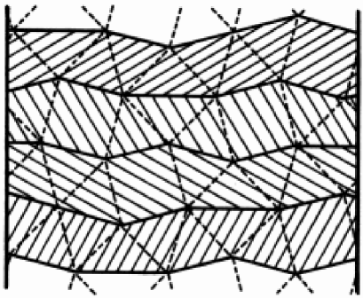
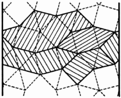
FIG. 1.: Dividing a strip of square-triangle tiling into layers. (a) ‘Slab’ approach (as used by [11]). (b) ‘Dead-surfaces’ approach (as used in the present paper for the 3D canonical-cell tiling.

FIG. 2.: Contour plot of the entropy as a function of the phason strain components $A_{1}$ and $A_{3}$ in the region of the maximum entropy.

REFERENCES

- [1] See P. A. Bancel in Quasicrystals: the State of the Art, P. J. Steinhardt and D. P. DiVincenzo (eds.), World Scientific, Singapore (1991), and references therein.
- [2] M. Boudard, M. de Boissieu, and C. Janot, J. Phys. C.M. 4, 10149 (1992).
- [3] M. Audier, M. Charre-Durand, and M. de Boissieu, Phil. Mag. B 68, 607 (1993).
- [4] R. Penrose, Bull. Inst. Math. and its Appl. 10, 2660 (1974); see also M. Gardner, Sci. Am. 236, No. 1, 110 (1977).
- [5] M. Widom in Proceedings of the Anniversary Adriatico Research Conference on Quasicrystals, M. V. Jarić and S. Lundqvist, World Scientific, Singapore (1990).
- [6] C. L. Henley, in Quasicrystals and Incommensurate Structures in Condensed Matter, M. J. Yacaman, D. Romeu, V. Castano, and A. Gómez (Eds.), World Scientific, (Singapore, 1990).
- [7] W. Li, H. Park, and M. Widom, J. Stat. Phys. 66, 1 (1992).
- [8] E. Cockayne, preprint (1994).
- [9] M. Widom, K. J. Strandburg and R. H. Swendsen, Phys. Rev. Lett. 58, 706 (1987); F. Lançon, L. Billard, and P. Chaudhari, Europhys. Lett. 2, 625 (1986).
- [10] K. J. Strandburg, L.-H. Tang, and M. V. Jarić, Phys. Rev. Lett. 63, 314 (1989).
- [11] Mark Oxborrow and C. L. Henley, J. Non-Cryst. Solids 153, 210 (1993); Phys. Rev. B 48, 6966 (1993).
- [12] L.-H. Tang, Phys. Rev. Lett. 64, 2390 (1990).
- [13] L. J. Shaw, V. Elser, and C. L. Henley, Phys. Rev. B 43, 3423 (1991).
- [14] K. J. Strandburg, Phys. Rev. B 44, 4644 (1991).
- [15] Mark Oxborrow, Ph. D. Thesis, Cornell University (1993).
- [16] M. Mihalkovič and P. Mrafko, Phil. Mag. Lett. 69, 85 (1994).
- [17] M. Mihalkovič, submitted to Phil. Mag. B.
- [18] M. Mihalković, W.-J. Zhu, M. E. J. Newman, M. Oxborrow, R. B. Phillips, and C. L. Henley, in preparation (1994).
- [19] J. Roth, J. Stadler, R. Schilling, and H.-R. Trebin, J. Non-Cryst. Solids, 153, 536 (1993); J. Harner and M. Krajĉí, Europhys. Lett. 13, 335 (1990).
- [20] H.-C. Jeong and P. J. Steinhardt, Phys. Rev. Lett. 73, 1943 (1994).
- [21] C. L. Henley in Quasicrystals: the State of the Art, P. J. Steinhardt and D. P. DiVincenzo (eds.), World Scientific, Singapore (1991).
- [22] M. Widom, Phil. Mag. Lett. 64, 297 (1991).
- [23] Y. Ishii, Phys. Rev. B 45, 5228 (1992).
- [24] M. E. J. Newman, C. L. Henley, and M. Oxborrow, to appear, Phil. Mag. B.
- [25] C. L. Henley, Phys. Rev. B 43, 993 (1991).
- [26] A preliminary report of the present work appeared in M. E. J. Newman and C. L. Henley, J. Non-cryst. Solids 153, 205 (1993).
- [27] E. Cockayne, preprint (1994).
- [28] M. Mihalkovič and M. Oxborrow, to appear in Aperiodic ’94, an International Conference on Aperiodic Crystals, G. Chapuis (ed.), World Scientific, Singapore (1995).
- [29] V. Elser, Phys. Rev. B 32, 4892 (1985).
- [30] Jarić, M. V., and Nelson, D. R., Phys. Rev. B 37, 4458 (1988).
- [31] This choice guarantees that, when expressed in Cartesian coordinates, the phason elastic tensor has a cyclic symmetry under permutations.
- [32] V. Elser in Proceedings of the XVth International Colloquium on Group Theoretical Methods in Physics, R. Gilmore (ed.), World Scientific, Singapore (1987).
- [33] C. L. Henley, J. Phys. A 21, 1649 (1988).
- [34] Notice that we use reduced (dimensionless) units of energy throughout, without showing temperature explicitly.
- [35] H.-C. Jeong and P. J. Steinhardt, Phys. Rev. B 48, 9394 (1993).
- [36] T. C. Lubensky in Aperiodicity and order, vol. 1, M. V. Jarić (ed.), (Academic Press, London, 1988).
- [37] M. V. Jarić, in Proceedings of the XVth International Colloquium on Group Theoretical Methods in Physics, ed. R. Gilmore, (World Scientific, Singapore, 1987).
- [38] However, so long as we have only a finite number of chemical potentials, we do not have the exactly correct ensemble. This caveat applies to all random tiling calculations where volume per layer is variable.
- [39] M. Widom, D. P. Deng, and C. L. Henley, Phys. Rev. Lett. 63, 310 (1989).
- [40] L. J. Shaw and C. L. Henley, J. Phys. A 24, 4129 (1991).
- [41] M. Widom, Phys. Rev. Lett. 70, 2094 (1993).
- [42] L.-H. Tang and M. V. Jarić, Phys. Rev. B 41, 4524 (1990).
- [43] P. A. Kalugin, J. Phys. A 27, 3599 (1994).
- [44] The term ‘dead surface’ was originally introduced by Onoda et al. [55] to describe a similar concept that arises in their growth algorithm for two-dimensional Penrose tilings. Our usage is slightly different since we are not generating a perfect quasiperiodic tiling obeying matching rules.
- [45] Our dead surface representation is reminiscent of a transfer-matrix approach to Ising models on lattices with spiral boundary conditions in which just one spin is added at a time [56], and has similar advantages.
- [46] In fact we implemented this part of the calculation as a chemical potential coupling to the packing fraction , rather than to directly, since the packing fraction is easier to evaluate. Since and are linearly related (see Ref. [25]), the two approaches are equivalent.
- [47] However, we can rule this out on other grounds: Oxborrow (unpublished) has discovered a finite polyhedron of cell faces which can be packed with tiles in two ways; hence, if just one configuration exists with a finite density of disjoint polyhedra of this kind, then the ensemble must contain all the ways in which the polyhedra can be repacked, and hence the entropy per unit volume must be at least .
-
[48]
There are various ways of extrapolating,
of course. The most successful are:
-
(i)
fitting the ratio : this obeys quite closely the form , yielding . (In recent experiments, de Boissieu [57] and co-workers have measured the anisotropy of the diffuse scattering surrounding the Bragg peaks for i(AlPdMn) and fitted their results to a model such as our having two independent elastic constants. They find values for these constants equivalent to , which is in fair agreement with this figure.) The value of is sufficient to determine a value . Unfortunately, is too ill behaved to be useful.
-
(ii)
extrapolating ; the factor of helps cancel out the trend denoted (ii) in the text.
-
(i)
- [49] This is only 40% of the value previously quoted by one of the authors in Refs. [21] and [6]. That earlier value was just the entry in the Table.
- [50] M. Baake, S. I. Ben-Abraham, R. Klitzing, P. Kramer, and M. Schlottman, Acta Crystallogr. A 50, 553 (1994).
- [51] An alternative way of comparing the two tilings is to apply the standard subdivision of the canonical-cell tiling into rhombohedra [25]. The entropy density of this sub-ensemble is where is the density of bonds, since each bond allows two local choices for subdivision into rhombohedra [25]. This comes out to only half of the total entropy of the unrestricted rhombohedron tiling [14]; on the other hand, the elastic constant is nearly the same for the two tilings. The “binary tiling” [9] also has nearly the same elastic constant as the unrestricted rhombus tiling, of which it is a subensemble [39].
- [52] This is not so surprising, since the govern the fluctuations of along the length of the tower in the direction, which are all sums of Fourier modes with parallel to .
- [53] M. V. Jarić and S.-Y. Qiu, Acta Crystallographica A 49, 576 (1993).
- [54] M. de Boissieu, P. Stephens, M. Boudard, C. Janot, D. L. Chapman, and M. Audier, Phys. Rev. Lett 72, 3538 (1994); J. Phys. Condens. Matt. 6, 10725 (1994).
- [55] G. Y. Onoda, P. J. Steinhardt, D. P. DiVincenzo and J. E. S. Socolar, Phys. Rev. Lett. 60, 2653 (1988); J. E. S. Socolar in Quasicrystals: the State of the Art, P. J. Steinhardt and D. P. DiVincenzo (eds.), World Scientific, Singapore (1991).
- [56] M. P. Nightingale in Finite-Size Scaling and Numerical Simulation of Statistical Systems, V. Privman (ed.), World Scientific, Singapore (1990).
- [57] M. de Boissieu, private communication.
- [58] M. Dzugutov, Phys. Rev. Lett. 70, 2924 (1993).