Ground-State Dynamical Correlation Functions: An Approach from Density Matrix Renormalization Group Method

Abstract

A numerical approach to ground-state dynamical correlation functions from Density Matrix Renormalization Group (DMRG) is developed. Using sum rules, moments of a dynamic correlation function can be calculated with DMRG, and with the moments the dynamic correlation function can be obtained by the maximum entropy method. We apply this method to one-dimensional spinless fermion system, which can be converted to the spin 1/2 Heisenberg model in a special case. The dynamical density-density correlation function is obtained.

Dynamical correlation functions of a model are of special interest, because they can provide a comprehensive comparison to experimental measurements. Unfortunately they are very difficult to calculate analytically or numerically for strongly correlated systems. Even for one-dimensional systems, the dynamical correlation functions are hard to obtain. For example the $S=1/2$ Heisenberg model, although its exact solution from Bathe Ansatz has been known for a long time, its ground-state dynamical correlation functions have not yet been obtained. Until now there are only a few general ways to obtain dynamical correlation functions. Analytically, only the asymptotic behavior of correlation functions for one-dimensional models in the quantum critical regime are able to obtain by bosonization or conformal field theory [1]. Numerically, one way to calculate dynamical correlation functions is the analytic continuation of quantum Monte Carlo simulations with the maximum entropy method [2, 3]. But this method will encounter essential difficulties if we are interested in zero-temperature properties. Another numerical method to calculate the ground-state dynamical properties [4] is based on the Lanczos method. The limitation of this method is that it cannot be applied to large systems.

The Density Matrix Renormalization Group (DMRG) method proposed by White [5] is a powerful method to study the ground state of one-dimensional interacting systems. With this method the ground state energy, a few excitation energies, and static correlation functions can be calculated for a large system. However, it was not clear if one can obtain dynamical properties from this method.

In this paper, we describe a numerical method for calculating ground-state dynamical correlation functions in a systematic way, which is a combination of DMRG and maximum entropy methods (MEM) [6]. In general the moments of a dynamical correlation function can be expressed as static correlation functions, which can be calculated by DMRG method. With these moments we can obtain the dynamic correlation function with MEM. We apply this method to the one-dimensional spinless fermion system with nearest neighbor interaction. This model is equivalent to the spin-1/2 $XXZ$ chain. We have considered two special cases of this model, corresponding to the $XY$ model and the Heisenberg model. The dynamical density-density correlation (namely the structure function $S(q,\omega)$ in spin chain) is obtained. For non-interacting case (the $XY$ model) we compare our result with the exact result, and obtain a very good agreement.

The one-dimensional spinless fermion model we consider has the following Hamiltonian:

$$H=-t\sum_{i}(c^{\dagger}_{i}c_{i+1}+{\hbox{h.c.}})+V\sum_{i}n_{i}n_{i+1},$$ (1)

where $c^{(\dagger)}_{i}$ are annihilation (creation) operators for a fermion at site $i$, and $n_{i}=c^{\dagger}_{i}c_{i}-\frac{1}{2}$. The Hamiltonian written in such form ensures the ground state is at half filling. This model may be mapped to the $XXZ$ model by the Jordan-Wigner transformation. Under this transformation $S^{z}_{i}=n_{i}$, $J_{x}=J_{y}=2t$, and $J_{z}=V$. At $V=0$ this model is equivalent to the $XY$ model, while at $V=2t$ it is equivalent to the Heisenberg model. We only consider these two cases in this paper, and the results for other $V$ will be presented elsewhere [7].

The first step of our method is to use sum rules to express the moments of a dynamical correlation function by some static correlation functions. The sum rules for the spin model have been derived [8]. We use the similar definition of the correlation functions as in Ref. [8]

$$\chi_{c}(q,t) = \frac{1}{2}\langle\{n(q,t),n(-q,0)\}\rangle-\langle n(q,t)\rangle\langle n(-q,0)\rangle,$$ (2)

$$\chi^{\prime\prime}(q,t) = \frac{1}{2}\langle[n(q,t),n(-q,0)]\rangle,$$ (3)

where $n(q)=N^{-1/2}\sum n_{l}e^{iql}$, the curly bracket is an anticommutator, and $\langle n(q)\rangle=$Tr$(n(q)e^{-\beta H})$. The fluctuation-dissipation theorem gives the relation: $\chi_{c}(q,\omega)=\coth(\omega/2k_{B}T)\chi^{\prime\prime}(q,\omega)$. The structure function or dynamic form factor $S(q,\omega)$ is defined as $S(q,\omega)=\chi^{\prime\prime}(q,\omega)/(1-e^{-\omega/k_{B}T})$. Due to the parity and time reversal symmetry in our model, $\chi^{\prime\prime}(q,\omega)$ and $\chi_{c}(q,\omega)$ have following properties: $\chi^{\prime\prime}(q,-\omega)=-\chi^{\prime\prime}(q,\omega)$ and $\chi_{c}(q,-\omega)=\chi_{(}q,\omega)$. At zero temperature $S(q,\omega)=\chi_{c}(q,\omega)=\chi^{\prime\prime}(q,\omega)$ for $\omega>0$, therefore the sum rules given in Ref. [8] can be written as

$$m_{1}(q) = \int^{\infty}_{0}\frac{d\omega}{\pi}\frac{\chi^{\prime\prime}(q,\omega)}{\omega}=\frac{1}{2}\chi(q,\omega=0)$$ (4)

$$m_{2}(q) = \int^{\infty}_{0}\frac{d\omega}{\pi}\omega\frac{\chi^{\prime\prime}(q,\omega)}{\omega}=\chi_{c}(q,t=0)$$ (5)

$$m_{3}(q) = \int^{\infty}_{0}\frac{d\omega}{\pi}\omega^{2}\frac{\chi^{\prime\prime}(q,\omega)}{\omega}=-\frac{1}{2}\langle[[H,n(q)],n(-q)]\rangle$$ (6)

$$= 2\langle c^{\dagger}_{i}c_{i+1}\rangle(1-\cos(q))$$ (7)

where $\chi(q,\omega=0)$ is the static susceptibility. These sum rules can be easily generalized to higher moments:

$$m_{l}(q) = \int^{\infty}_{0}\frac{d\omega}{\pi}\omega^{n-1}\frac{\chi^{\prime\prime}(q,\omega)}{\omega}$$ (8)

$$= \left\{\begin{array}[]{rl}-\frac{1}{2}\langle[[H,...,[H,n(q)]...],n(-q)]\rangle&\hskip 7.22743ptl\hskip 7.22743pt$ even$\\ \frac{1}{2}\langle\{[H,...,[H,n(q)]...],n(-q)\}\rangle&\hskip 7.22743ptl\hskip 7.22743pt$ odd$\end{array}\right..$$ (11)

Apart from the first moments which is given by the static susceptibility, all the other moments can be expressed as equal-time correlation functions. Theoretically if all the moments are known, one can obtain the $\chi^{\prime\prime}(q,t)$ and thus $\chi^{\prime\prime}(q,\omega)$. In real calculations, it is tedious to calculate the commutators for higher moments, and there are more and more new equal-time correlation functions appear in the expression of higher moments. However it is still reasonable to obtain the expression for the first several moments using a symbolic manipulator, such as Mathematica, to calculate the commutators. In this work we have calculated the expressions for the first five moments. Details of the expressions for the fourth and fifth moments will be given elsewhere [7].

The second step is to obtain the moments by calculating those static correlation functions with DMRG. The infinite lattice method (see Ref. [5] for details) is used in our calculations for open ended chains. $t=1$ is chosen, and states kept at each iteration varies from 52 to 64. We calculate the equal-time correlations, for example $\langle n_{i}n_{j}\rangle$, by taking $j$ in the middle of the system. For a system which has parity and translational symmetries, $\langle n_{j}n_{i}\rangle$ only depends on $|i-j|$. Therefore $\langle n_{q}n_{-q}\rangle=\sum_{l}\langle n_{j}n_{j+l}\rangle e^{iql}$ is independent of $j$. Since the calculations are done with open boundary condition, $\langle n_{j}n_{j+l}\rangle$ depends on the position $j$. The boundary effect is larger when $j$ or $j+l$ is closer to boundary, therefore we choose $j$ at the center of the system. Also due to the open boundary, the correlation $\langle n_{j}n_{j+l}\rangle$ has an even-odd oscillation in $j$. We take the mean value of $\langle n_{j}n_{j+l}\rangle$ at $j$ even and odd, which is close to the value with period boundary condition for a system having the same size. When the system size goes to infinity, the boundary effect can be neglected. We calculate the moments for system sizes varying from 100 sites to 200 sites, and obtain their values for infinite system by extrapolating the data.

The next step is to use MEM to obtain the dynamical correlation functions. MEM has become standard way to extract maximum information from incomplete data [6]. This method has been applied to the analytic continuation of the Quantum Monte Carlo data [9], and in this paper we apply a similar method to extract the dynamic susceptibility $\chi^{\prime\prime}(q,\omega)$ from the finite number of moments $m_{l}$ with the corresponding errors $\sigma_{l}$. Defining $f(\omega)=\chi^{\prime\prime}(\omega)/\omega$, which is a positive definite, as the distribution function, and the entropy or the information function $S=\sum_{\omega}f(\omega)-f(\omega)\log f(\omega)$. By maximizing the entropy under the constrains $m_{l}-\int_{0}^{\infty}\frac{d\omega}{\pi}\omega^{l-1}f(\omega)=0$, $f(\omega)$ has the following form

$$f(\omega)=e^{-\sum_{l=1}^{n}(\lambda_{l}\omega^{l-1})},$$ (12)

where $n$ is the number of moments and $\lambda_{l}$ are the Lagrange multipliers. At this point one may try to find $\lambda_{l}$ by requiring the $f(\omega)$ to satisfy the constrains without considering the error bars of the moments. However, in general, the error bars cannot be neglected. The kernel of the transformation is singular, so small error bars in moments may produce large errors in $f(\omega)$. By maximizing the posterior probability $e^{\alpha S-L}$ where $L\equiv\sum_{l}(m_{l}-\int_{0}^{\infty}\frac{d\omega}{\pi}\omega^{l-1}f(\omega))^{2}/\sigma_{l}^{2}$, one can find the most probable $f(\omega)$, which gives us the moments within the range of error bars.

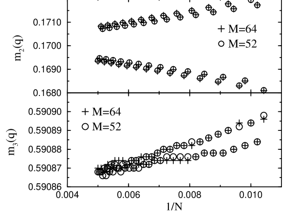
Let us first discuss the extrapolation and the error bar of our DMRG results. There are two major contributions to the error: that from finite size effects and that from basis set transaction in the DMRG calculations. The error bar of DMRG calculation for any finite size is obtained by varying the number of states kept at each iteration, whereas the finite size error is obtained by varying the system size. The asymptotic behavior of correlation functions is known for this model [1], which decay as a power of system size. For a system with a gap, the extropolation should be done as an exponential function of system size. In Fig. 1, we plot the second and third moments at $q=\pi/2$ for $V=2t$ as a function of $1/N$, where $N$ is the number of sites of the system. The error from basis set transaction produces the error in the extrapolating values. We use this resultant error to estimate the error bar of the moments. Extrapolating to $1/N\rightarrow 0$ gives $m_{2}=0.1700$, and the error bar is estimated as $10^{-4}$. For the third moment we have $m_{3}=0.59085$ and the estimated error bar is $2\times 10^{-5}$. Actually the third moment is known exactly: $m_{3}=-\frac{2}{3}E(1-\cos(q))$ with the ground state energy per site $E=-2(\ln 2-1/4)$. The exact value at $\pi/2$ is 0.590863.

We test our method for the non-interacting case. In this case, $\chi^{\prime\prime}(q,\omega)$ is known exactly:

$$\chi^{\prime\prime}(q,\omega)=\frac{\theta(\omega-2t|\sin(q)|)\theta(4t|\sin(q/2)|-\omega)}{[16t^{2}\sin^{2}(q/2)-\omega^{2}]^{1/2}},$$ (13)

where $\theta(x)$ is the step function. The moments can also be calculated analytically. In Table I, we compare the moments calculated by DMRG with the exact results. The error bars obtained by DMRG provide a very good estimation. Apart from the five moments, there are two more pieces of information in this case: the energy boundaries $2t|\sin(q)|<\omega<4t|\sin(q/2)|$ for $\chi^{\prime\prime}(q,\omega)$. Using the MEM, we obtain $\chi(q,\omega)$ for $q=2\pi/3$. In Fig. 2, we plot $\chi(q,\omega)$ obtained by MEM with different number of moments and the exact one from Eq. (5). It shows that the $\chi(q,\omega)$ obtained by MEM converge to the exact one when the number of moments is increased, and $\chi(q,\omega)$ calculated with five moments is a good approximation for the exact result. We have also calculated $\chi(q,\omega)$ for other $q$, they have similar behavior.

For the interacting case with $V=2t$, which corresponding to the Heisenberg model, the elementary excitations are known as $S=1/2$ objects [10] (spinons). The dispersion relation is $\epsilon(q)=\pi t|\sin(q)|$ [11], which provides the lower bound of excitation energies for each momentum $q$. The spectral weight is dominated by the continuum of the two-spinon excited states [12], and the energy range for the continuum is $t\pi|\sin(q)|<\omega<2t|\pi\sin(q/2)|$. Since the contributions from the excited states of more than two spinons are finite, we only have the low energy bound. In Fig. 3, the $\chi^{\prime\prime}(q,\omega)$ obtained by MEM with different number of moments are plotted for $q=2\pi/3$. One can see the tendency of the curves as the number of moments increase. $\chi^{\prime\prime}(q,\omega)$ tends to diverge at lower-bound. In Fig. 4, $\chi^{\prime\prime}(q,\omega)$ is plotted for other momentums. We marked the position of upper-bound for two-spinon excited states. It is obvious that the contributions from excited states with more than two spinons are finite, although they are small.

In conclusion, we have developed a numerical method for calculating the ground-state dynamical correlation functions in one-dimensional quantum systems based on the Density Matrix Renormalization Group Method and the maximum entropy method. We demonstrate this method on the dynamical density-density correlation $\chi^{\prime\prime}(q,\omega)$ of the spinless fermion system with nearest neighbor interaction. For the non-interacting case, it corresponds to the $XY$ model, and the dynamical density-density correlation function obtained by our method shows a very good agreement with the exact result. For the interacting case with $V=2t$, it corresponds to the Heisenberg model, we obtain the $\chi^{\prime\prime}(q,\omega)$, which was not known before. This method is a very general one, which can be applied to any one-dimensional system with short range interaction like, e.g. the Hubbard model, the $S=1$ Heisenberg model, the interacting fermion (or boson) system with randomness.

We would like to acknowledge useful discussions with J.E. Gubernatis, Shoudan Liang, and R.N. Silver. This work was supported by the National Science Foundation grant No. DMR-9107563. In addition MJ would like to acknowledge the support of the NSF NYI program.

FIG. 1.: Moments versus the inverse system size $1/N\rightarrow 0$ for $V=2t$ and $q=\pi/2$, where $M$ is the number of states kept at each iteration in DMRG calculations. The extropolation is to $1/N\rightarrow 0$, and the error is estimated by the different extropolations caused by the errors in slope.

FIG. 2.: The dynamical structure function $\chi^{\prime\prime}(q,\omega)$ for $V=0$ (the $XY$ model) and $q=2\pi/3$. We plot the results obtained by MEM with different number of moments. Two solid vertical lines are the energy boundaries.

FIG. 3.: The dynamical structure function $\chi^{\prime\prime}(q,\omega)$ for $V=2t$ (the Heisenberg model) and $q=2\pi/3$. We plot the results obtained by MEM with different number of moments. The solid vertical line is the lower boundary. The arrow marks the position of the upper boundary for the two-spinon excited states.

FIG. 4.: The dynamical structure function $\chi^{\prime\prime}(q,\omega)$ for $V=2t$ (the Heisenberg model) at (a) $q=\pi/2$, and (b) $\pi/3$ and $\pi/4$. $\chi^{\prime\prime}(q,\omega)$ are obtained by MEM with five moments. The solid vertical lines are the lower boundaries for each momentum. The arrow marks the position of the upper boundary of the two-spinon excited states.

TABLE I.: The comparison of the moments obtained by DMRG with the exact results for $V=0$ and $q=2\pi/3$. In the DMRG calculations 64 states are kept at each iteration, and the error bars are estimated by changing the number of states kept and finite size scaling.

	EXACT	DMRG	ERROR
$m_{1}(2\pi/3)$	0.121013	0.1211	$1\times 10^{-3}$
$m_{2}(2\pi/3)$	0.333333	0.33337	$5\times 10^{-5}$
$m_{3}(2\pi/3)$	0.954930	0.954928	$5\times 10^{-6}$
$m_{4}(2\pi/3)$	2.826993	2.8273	$5\times 10^{-4}$
$m_{5}(2\pi/3)$	8.594367	8.59434	$5\times 10^{-5}$

REFERENCES

- [1] A. Luther and I. Peschel, Phys. Rev. B12, 3908 (1975); I. Affleck in Fields, Strings and Critical Phenomena, Ed. E. Brezin and J. Zinn-Justin (North Holland, Amsterdam, 1990).
- [2] J. Deisz, M. Jarrell and D. L. Cox, Phys.Rev. B42, 4869 (1990).
- [3] R. Preuss, A. Muramatsu, W. von der Linden, P. Dieterich, F. F. Assaad, and W. Hanke, Phys. Rev. Lett. 73, 732 (1994).
- [4] E. R. Gagliano and C. A. Balseiro, Phys. Rev. Lett. 59, 2999 (1987).
- [5] S. R. White, Phys. Rev. Lett. 69, 2863 (1992), Phys Rev. B48, 10345 (1993).
- [6] T. Brandt, Statistical and Computational Methods in Data Analysis, (North-Holland, Amsterdam, 1983), chap. 13; S.F. Gull and J. Skilling, IEE Proceedings 131, 646 (1984); R.K. Bryan, Eur. Biophys. J. 18, 165 (1990).
- [7] Hanbin Pang, H. Akhlaghpour, and M. Jarrell, unpublished.
- [8] P. C. Hohenberg and W. F. Brinkman, Phys. Rev. B10, 128 (1974).
- [9] R.N. Silver, D.S. Sivia, J.E. Gubernatis, and M. Jarrell, Phys. Rev. Lett. 65, 496 (1990); J.E. Gubernatis, M. Jarrell, R.N. Silver, and D.S. Sivia, Phys. Rev. B44, 6011 (1991).
- [10] L. D. Faddeev and L. A. Taktajan, Phys. Lett. 85A, 375 (1981).
- [11] J. des Cloizeaux and J. J. Pearson, Phys. Rev. 128, 2131 (1962).
- [12] G. Müller, H. Beck, and J. Bonner, Phys. Rev. Lett. 43, 75 (1979).