Replica Theory and Large $D$ Josephson Junction Hypercubic Models

Abstract

We study the statistical mechanics of a $D$-dimensional array of Josephson junctions in presence of a magnetic field on a lattice of side $2$. In the high temperature region the thermodynamical properties can be computed in the limit $D\to\infty$. A conjectural form of the thermodynamic properties in the low temperature phase is obtained by assuming that they are the same of an appropriate spin glass system, based on quenched disordered couplings. Numerical simulations show that this conjecture is very accurate in one regime of the magnetic field, while it is probably slightly inaccurate in a second regime.

cond-mat 9502067

1 Introduction

In this paper we pursue our research program on the relation among systems based on a Hamiltonian containing quenched disorder and systems with a fixed frustrated but non-random Hamiltonian [1, 2]. Here we study the statistical mechanics of arrays of Josephson junctions [3] in $D$-dimensions, in the limit where $D\to\infty$ on a lattice of size $2$ (i.e. on a single hypercube with $2^{D}$ points). The case of a fully frustrated lattice has been already discussed in reference [4].

In the framework of the spherical approximation the thermodynamic properties can be computed by using the results obtained in [3]. It is possible to prove that the spherical approximation gives the correct results even for the XY model (the one that will mainly interest us here) in the high temperature phase. At $T=T_{c}$ the system undergoes a phase transition. In the low temperature region the spherical approximation breaks down. We conjecture that the thermodynamical properties of the system are the same of an appropriate spin glass model, constructed in such a way to have the same high temperature expansion than the original deterministic model. We solve the disordered model by using the replica approach.

We have simulated numerically systems in dimension $D$, ranging from $3$ to $16$. We find that the comparison of the numerical simulation with the theoretical results is extremely good in the high temperature phase (as expected). In the low temperature phase things seem to work quite well when we move toward the fully frustrated model (starting from a magnetic field $\theta=\frac{\pi}{2}$ and increasing $\theta$), but when decreasing $\theta$ (towards the ferromagnetic system) we find a rather disturbing phenomenon. Indeed in this region a naive extrapolation for $D\to\infty$ gives a result which differs slightly from the analytic results (obtained by applying replica theory to the model which contains quenched disorder). Such discrepancy becomes larger and larger when decreasing the frustration. We are unable to decide if in this regime our analytic results are only a good approximation to the behavior of the system without quenched disorder, or if they are exact and the finite $D$ corrections have a peculiar dependence on $D$. An analytic computation inside our theoretical framework of the $1\over D$ corrections would be extremely useful, but it goes beyond the aims of this note.

In section (2) we give a short summary of the results obtained in [3]. In section (3) we describe our strategy, and define the model with quenched disorder which we will substitute to the original deterministic model. In section (4) we will discuss the high $T$ expansion. In section (5) we will use replica theory to solve the random model for $T<T_{c}$. In section (6) we will describe our numerical simulations, and compare them to the analytic results obtained in the former sections. Finally in the appendix we close a gap in the proof of ref. [3] about the connection of the high temperature expansion and the Green functions of the $q$-deformed harmonic oscillator.

2 Diagram Counting, Josephson Junctions and $q$-Deformations

We will start here by defining the relevant statistical models, and by reviewing in a very cursory manner the results of [3]. The prototype model is the Gaussian model, defined by the Hamiltonian

$$\beta H_{G}\equiv-\beta\Re\{c(D)\sum_{j,k}\eta^{*}_{j}U_{j,k}\eta_{k}\}+\frac{1}{2}\sum_{k}|\eta_{k}|^{2}\ .$$ (1)

Here $c(D)$ is a normalization constant, which will be useful later to rescale the Hamiltonian in order to obtain a non trivial limit when $D$ goes to infinity. $c(D)$ will be $\frac{1}{2D}$ for the usual ferromagnetic XY model (and in this case we will get a phase transition at $\beta=1$). For a model with random couplings, and for the frustrated models we will be mainly discussing in this note, we will have to take $c(D)\simeq(2D)^{-\frac{1}{2}}$ in order to insure a sensible infinite dimensional limit .

Real and imaginary part of the complex $\eta_{j}$ lattice variables can take values that range from $-\infty$ to $+\infty$. We will consistently indicate with $\eta$ the fields of the Gaussian model. With $\phi_{i}$ we will denote the fields of the XY model, which are constrained to be, on every site, of modulus $1$, i.e. for all sites $i$

$$\ |\phi_{i}|^{2}=1\ .$$ (2)

Their dynamics is governed by the Hamiltonian

$$\beta H_{XY}\equiv-\beta\Re\{c(D)\sum_{j,k}\phi^{*}_{j}U_{j,k}\phi_{k}\}\ .$$ (3)

With $\sigma_{i}$ we will denote the fields of the spherical model, which satisfy the constraint

$$\sum_{i}|\sigma_{i}|^{2}=N\ ,$$ (4)

with the Hamiltonian

$$\beta H_{S}\equiv-\beta\Re\{c(D)\sum_{j,k}\sigma^{*}_{j}U_{j,k}\sigma_{k}\}\ .$$ (5)

We can rewrite the spherical model Hamiltonian by including the constraint by means of a Lagrange multiplier $\mu$. We can write

$$\beta H_{S}\equiv-\beta\Re\{c(D)\sum_{j,k}\sigma^{*}_{j}U_{j,k}\sigma_{k}\}+\mu(\sum_{i}|\sigma_{i}|^{2}-N)\ ,$$ (6)

for unconstrained variables. Integration over $\mu$ insures that the spherical constraint is implemented.

The $U$ couplings are non-zero only for first neighboring site couples. They are complex numbers of modulus $1$. In the following we will always have that

$$U_{j,i}=U^{*}_{i,j}\ ,$$ (7)

i.e. the link couplings are oriented, and when coming back on a link one takes the opposite phase of when following it in the positive direction. By using the language of gauge theories one says that the $U$ couplings are $U(1)$ lattice gauge fields [5].

We will be discussing here hypercubic models. For a $D$ dimensional model the field variables live on a $D$-dimensional hypercube, which is done of $2^{D}$ points. We only include link couplings which are internal to the cube, i.e. we use open boundary conditions. The number of independent link couplings in our lattice is $D2^{D-1}$. The limit $D\to\infty$ is taken by letting the dimensionality of the hypercube to increase.

Apart from the two cases we already quoted (i.e. the ferromagnetic model with all $U$ fields equal to $1$ and the XY spin glass, where $U_{j,k}=\exp(ir_{j,k})$, and the $r_{j,k}$ are random numbers uniformly distributed in the interval $(0,2\pi]$) we will mainly be interested here in models where the couplings are such to generate a constant magnetic field $\theta$. The magnetic field which flows to a given elementary plaquette ${\cal P}$ is

$$\prod_{\cal P}U_{\cal P}=e^{\pm i\theta_{\cal P}}\ ,$$ (8)

where the sign of the exponents determine if the field is flowing in the positive or in the negative direction. We will be interested in the case where $\theta_{\cal P}=\theta$ is constant on all the lattice, i.e. the plaquettes undergo a constant, uniform frustration. The case $\theta=0$ gives the ferromagnetic model, while the case $\theta=\pi$ gives the fully frustrated model, which we have discussed in detail in ref. [4]. If we let $\theta_{\cal P}$ to be a random variable we obtain a so-called gauge glass [6, 7, 8].

The values of the signs of the exponents that enter eq. (8) are in part arbitrary. Parallel plaquettes have to be cut by a flux flowing in the same direction, i.e. the signs must have the structure ${\cal S}_{\alpha,\beta}$, where ${\cal S}$ is a tensor, which is automatically antisymmetric because of the way we have used to define the $U$ fields. We are interested in the choice of a generic structure of ${\cal S}$ (for the reasons we have discussed in [1, 2] and we will discuss better in the following). We need a generic representative of the ensemble of the possible choices of ${\cal S}$. One can see that for $D>3$ the choice ${\cal S}_{\alpha,\beta}=1$ is not a good choice (this is not true in $3$ and $2$ $D$, where all choices of ${\cal S}$ are equivalent). We also need to define the parameter

$$q\equiv\cos(\theta)\ ,$$ (9)

which will play an important role in the following.

Let us be more explicit and summarize. Our model lives in a magnetic field given by the antisymmetric tensor

$$\theta_{\alpha,\beta}={\cal S}_{\alpha,\beta}\ \theta\ ,$$ (10)

where in the continuum $\theta_{\alpha,\beta}$ becomes $\partial_{\alpha}A_{\beta}-\partial_{\beta}A_{\alpha}$. This is a condition of complex frustration on the elementary plaquettes. For $\theta=\pi$ we recover the fully frustrated model. On our hypercubic lattice the construction of the $U$ fields that generate a $\theta$ frustration is unique modulo gauge transformations, and can be easily given. We define $U_{\mu}(j)$ the coupling $U$ which goes from the site $j$ in the direction $\mu$ (we only have first neighbor non-zero coupling). $\mu$ goes from $1$ to $D$, since we only need to set couplings in the positive direction (the one going in the negative direction are set by the relation (7)). We set

$$U_{1}(j)=1\ ,$$ (11)

and for $\mu>1$

$$U_{\mu}(j)=e^{i\theta\sum_{\nu=1}^{\mu-1}{\cal S}_{\mu,\nu}j_{\nu}}\ .$$ (12)

For example in $4$ dimensions we get

$$U_{1}(j) = 1\ ,$$

$$U_{2}(j) = e^{i\theta({\cal S}_{2,1}j_{1})}\ ,$$

$$U_{3}(j) = e^{i\theta({\cal S}_{3,1}j_{1}+{\cal S}_{3,2}j_{2})}\ ,$$

$$U_{4}(j) = e^{i\theta({\cal S}_{4,1}j_{1}+{\cal S}_{3,2}j_{2}+{\cal S}_{3,3}j_{3})}\ .$$

In this note we will obtain a generic ${\cal S}$ by picking up at random the $\pm 1$ components of the antisymmetric tensor ${\cal S}_{\alpha,\beta}$. This is only a small amount of randomness. The system is determined by $D\ 2^{D-1}$ couplings, i.e. a number of couplings exponentially large in $D$, while we are using only order of $D^{2}$ random numbers to pick up phases which make generic the magnetic field tensor. It is maybe possible to imagine simple forms of the tensor ${\cal S}$ which give a generic magnetic field (i.e. with the correct moments).

Let us start from the discussion of the gaussian model, where the $\eta$ fields are unconstrained, (1), and summarize the steps taken in ref. [3]. We will later introduce the modifications needed to discuss the XY (2,3) and the spherical model (4,5). We will assume in the following we are taking the $D\to\infty$ limit by the hypercubic lattice approach we have described before.

On general grounds the free energy $F$ of a statistical model like the ones we have defined in (1,3,5) can be written through its high temperature expansion as [9]

$$\beta F(\beta)=\sum_{n}\frac{(\beta c(D))^{n}}{n}\ {\cal N}(n)\ \langle W(C)\rangle_{n}\ ,$$ (13)

where the sum runs over all circuit lengths $n$, ${\cal N}(n)$ is the number of rooted closed circuits of length $n$, and $\langle W(C)\rangle_{n}$ is the average over all circuits of length $n$ of the value of Wilson loop $W(C)$ (defined as the oriented product of the couplings that one encounters when following the closed circuit). We will be interested in the $D\to\infty$ limit, and define

$$G^{(q)}_{n}=\lim_{D\to\infty}(2D)^{-\frac{n}{2}}{\cal N}(n)\ \langle W(C)\rangle_{n}\ .$$ (14)

We are indicating with the superscript $(q)$ the dependence of $G$ over the value of $\theta$, i.e. of $q$. Using this definition in the $D\to\infty$ limit the free energy reads

$$\beta F(\beta)=\sum_{n}\frac{\beta^{n}G^{(q)}_{n}}{n}\ .$$ (15)

In order to obtain the free energy of the system we will have to compute the functions $G^{(q)}_{n}$.

In the ferromagnetic case (where $\theta=0$ and $q=1$) everything is easy, since $\langle W(C)\rangle_{n}=1$ for all values of $n$. Here it is easy to recover all the usual results of the high $T$ expansion in the $D\to\infty$ limit [3].

The next step can be started by discussing the $D\to\infty$ limit of a gaussian, XY or spherical spin glass, i.e. the situation where $U_{j,k}=\exp(ir_{j,k})$, and the $r_{j,k}$ are random numbers uniformly distributed in the interval $(0,2\pi]$, and one eventually averages over the $r$ random variables. We have already reminded the reader that this is an usual spin glass (the replica symmetric solution for the XY case is discussed already in [10]). This is not one of the non-random models that we want to study here, but we are using it just in order to go back soon to our models in magnetic field $\theta$ with a bit more knowledge. In this case one can easily see that the only (closed) diagrams contributing to the free energy are backtracking diagrams. For any steps going to $i$ to $j$ we need the opposite step going from $j$ to $i$, or the integrals over the quenched $r$ variables gives us zero.

This step is completed by noticing that the backtracking diagrams are also the only ones which survive (in the $D\to\infty$ limit) in the $\theta=\frac{\pi}{2}$ model, which we call half frustrated. Here on all elementary plaquettes the product of the plaquette couplings is purely imaginary, $\pm i$. It is easy to see why. In the $D\to\infty$ limit each step is taken in a different direction. So each time we find a phase $i$ which enters our Wilson loop, we will have to consider the contribution of an other path with the conjugate phase $-i$ (in $D$ finite two steps in the same direction can create a situation where this cancellation does not hold anymore).

In this way we have associated backtracking diagrams to one particular case of our frustrated models, the one in which $\theta=\frac{\pi}{2}$, and the plaquette frustration has the constant imaginary value $i$ (apart from a sign). The next step consists of associating to each backtracking diagram a planar diagram.

The instructions are the following. In order to compute $G^{(0)}_{2n}$ consider $2n$ letters, equal at couples, i.e. take two $a$, two $b$, two $c$, up to $n$ couples. Form a word by ordering these letters, and put the ordered letters on a circle. Now connect equal letters with lines. Count the number of intersections of these lines. Call $I_{n}(m)$ the number of words done of $n$ couples which have $m$ intersections. $I_{n}(m)$ is a topological invariant, and depends only on the order of the letters. The condition of zero intersections implies that the diagram is planar. One has that, for the Gaussian model,

$$G^{(0)}_{n}=I_{n}(0)\ .$$ (16)

This shows [3] that the problem of the gaussian half-frustrated model (and of the Gaussian spin glass) is solved by counting planar diagrams. $I_{n}(0)$ has been computed in [11], and the generalization to the XY and spherical model is straightforward.

The next step of the deduction of ref. [3] is the one that concerns our model which lives in a constant magnetic field. It is a generalization of the counting argument discussed before, and it says that we can solve our problem by counting non-planar diagrams, i.e. by counting words which have a non-zero number of intersections. There are two crucial results. The first states that, in a large number of dimensions $D$,

$$G^{(q)}_{2n}=\sum_{w(2n)}q^{A(w(2n))}\ ,$$ (17)

where $A(w)$ is the signed area associated to the diagram represented by the word $w$. Planar diagrams, with zero intersections, have zero area. In the $D\to\infty$ limit all the steps which form the diagram are taken in different directions, and the projected signed area over the plane $(\mu,\nu)$ $A_{\mu,\nu}$ can only take the values $0$ and $\pm 1$. The total area $A$ has been defined as the sum of the modulus of the individual signed areas

$$A\equiv\sum|A_{\mu,\nu}|\ .$$ (18)

The second part of this step shows that $A(w)$ is equal to the number of intersections of the line drawing associated to the word $w$. Considering diagrams which have a non-zero area means considering words which line drawing has a non-zero number of intersections.

This generalization of the counting of planar diagrams to a counting on non-planar diagrams has shown in a last step to have an underlying powerful algebraic structure. Indeed ref. [3] shows that (and we complete here the proof of this statement)

$$G^{(q)}_{2n}=\sum_{w(2n)}q^{A(w(2n))}=\langle 0|\ {\cal X}_{q}^{2n}|0\rangle\ ,$$ (19)

where the operator ${\cal X}_{q}$ is

$${\cal X}_{q}={\cal R}_{q}+{\cal L}_{q}\,$$ (20)

and the operators ${\cal L}_{q}$ and ${\cal R}_{q}$ satisfy the commutation relations of the annihilation and the creation operators of a $q$-deformed harmonic oscillator

$${\cal L}_{q}{\cal R}_{q}-q{\cal R}_{q}{\cal L}_{q}=1\ .$$ (21)

The vacuum state $|0\rangle$ (for the model with charge $q$) is defined by the condition

$${\cal L}_{q}|0\rangle=0\ .$$ (22)

${\cal L}_{q}$ may be identified with the annihilation operator and $R_{q}$ with the creation operator for a $q$-deformed harmonic oscillator. They can be represented as:

$${\cal R}_{q}|m\rangle = [m]_{q}^{\frac{1}{2}}|m+1\rangle\ ,$$

$${\cal L}_{q}|m\rangle = [m-1]_{q}^{\frac{1}{2}}|m-1\rangle\ ,$$ (23)

where

$$[m]_{q}\equiv\frac{1-q^{m+1}}{1-q}\ ,$$ (24)

and $m$ takes integer values in the interval $(0-\infty]$.

For $q=1$ we have the usual ferromagnet, for $q=-1$ the fully frustrated model [4], and for $q=0$ our half frustrated model (which has the same diagrammatic expansion than the spin glass model).

These are the basis on which we will try to build here, mainly trying to gather information about the behavior of these frustrated models in the low $T$, glassy phase.

3 Our Strategy and the Definition of the Random Model

We will use here a strategy we have introduced in [1], [2] (see also [12] for the development of very connected ideas). We start with a model which does not contain quenched disorder, but that is complex enough to make us suspicious of the possible presence of a spin glass like phase for temperatures $T$ low enough. We look for a model which contains quenched disorder, and that is similar enough to the original model to have potentially the same behavior (even in the low $T$ phase, if we are very ambitious). Replica theory allows us to solve the random model, and to try and get information about the deterministic model. References [1] and [2] discuss successful examples of the use of this strategy.

Here we will adopt the same approach. We will introduce a model containing random quenched disorder. In this new model the new $\widehat{U}$ couplings will be chosen at random (as opposed to the original $U$ couplings which are determined by the deterministic algorithm (12) such to give us the needed complex frustration). The random values of the $\widehat{U}$ will be selected, following [2], such that the new free energy will have the same high temperature expansion than the original model. So, we will be in the typical situation described in [1] and [2]. We will have a model where the couplings $\widehat{U}$ will be distributed according to a probability distribution, determined from the request of finding the same high $T$ expansion than in the original frustrated model. The original model will be in this way by construction a given (hopefully typical) realization of the coupling constants constructed according to this probability distribution.

Because of these remarks, and of our constructive procedure, the deterministic model and the random one coincide in the high $T$ phase. We hope to learn as much as possible about the low $T$ phase, and that the two models are also in this phase very similar.

We will have to start by computing the high temperature expansion for our model with complex frustration. Knowing that we will use a reverse engineering procedure in order to find out the probability distribution of random couplings $\widehat{U}$ that have the same high temperature expansion. Finally we will use the replica theory to compute the low temperature behavior of the random model. For sake of simplicity we will present here the computation done under the hypothesis of no replica symmetry breaking. We will compare these analytic results to numerical simulations of the frustrated model.

We will consider a model containing quenched disorder that has the same form of the original model with complex deterministic frustration. In the random model the couplings $\widehat{U}$ will be taken randomly among all matrices having the same spectral distribution of the deterministic model. More precisely for finite $D$ we extract a set of $2^{D}$ values of the eigenvalues $\lambda$, such that

$$2^{-D}\sum_{j=1,2^{D}}\lambda_{j}^{n}\simeq\int d\lambda\ \rho_{\Delta}(\lambda)\ \lambda^{n}\ ,$$ (25)

where $\rho_{\Delta}$ is the spectral density of the Laplacian operator, and will be discussed in more detail in next section. We finally set

$$\widehat{U}_{i,k}=\sum_{j=1,2^{D}}V^{*}_{i,j}\ \lambda_{j}\ V_{j,k}\ ,$$ (26)

where $V$ is a random unitary matrix i a $2^{D}$ dimensional space.

4 The High Temperature Expansion

We have explained that we will construct the model based on the random couplings $\widehat{U}$ by requiring that the high $T$ expansion is the same than in the original model with complex frustration (and no disorder). Let us remark that both these models, the random one and the deterministic one, are regular, i.e. there are no couplings of $O(1)$ when $D\to\infty$. In other words all the $U$ couplings and the $\widehat{U}$ ones, after being multiplied times the appropriate $c(D)$ factor, go to zero in this limit. Under this condition the high temperature expansion for the XY model (defined in (2,3)) is equal to the one of the spherical model ((4,5)). One can verify this statement by checking that in the two cases (i.e. for the spherical and for the XY model) the same diagrams survive in the $D\to\infty$ limit. The regularity condition guarantees the absence of diverging couplings which could break the equivalence.

Thanks to this result we will be able to start from computing the high $T$ expansion of the spherical model ((4,5)), in order to work out results valid for the XY model (which is the one we study numerically). That will make our task far easier.

We introduce the Laplacian operator $\Delta$ defined as

$$(\Delta f)_{j}\equiv\sum_{k}U_{j,k}f_{k}\ ,$$ (27)

We denote its spectral density by $\rho_{\Delta}(\lambda)$, and we express the trace of its $n$-th moment as

$$2^{-D}\ \mbox{Tr}(\Delta^{n})=\int d\lambda\ \rho_{\Delta}(\lambda)\ \lambda^{n}\ .$$ (28)

Here the trace is taken over a space of dimensionality $2^{D}$, and the normalizing factor $2^{-D}$ is such that the spectral density of the identity operator $\rho_{1}(\lambda)$ is $\delta(\lambda-1)$.

We start by remarking that the internal energy density of the Gaussian model is given in terms of $\rho_{\Delta}(\lambda)$ by

$$E_{G}=\int\ d\lambda\ \rho_{\Delta}(\lambda)\ \frac{\lambda}{1-\beta\lambda}\ .$$ (29)

By using the expression of the Hamiltonian which includes the spherical constraint, (6), we see that analogously to (29) we find

$$E_{S}=\int\ d\lambda\ \rho_{\Delta}(\lambda)\ \frac{\lambda}{\mu(\beta)-\beta\lambda}\ ,$$ (30)

where $\mu$ is a function of $\beta$. It is fixed by the condition

$$\int d\lambda\ \rho_{\Delta}(\lambda)\ \frac{1}{\mu(\beta)-\beta\lambda}=1\ ,$$ (31)

which tells that $\langle\sum_{i}|\sigma_{i}|^{2}\rangle=N$, i.e. that the $\sigma$ variables satisfy the spherical constraint (4).

Equations (30,31) can be written in a more compact form as

$$\mu(\beta) = R(\frac{\beta}{\mu(\beta)})\ ,$$ (32)

$$E(\beta) = \frac{\mu-1}{\beta}\ ,$$ (33)

where the function $R$ is given by

$$R(z)=\int d\lambda\ \rho_{\Delta}(\lambda)\ \frac{1}{1-z\lambda}\ .$$ (34)

One uses (32) to determine $\mu$, and inserting it in (33) one determines the internal energy density of the system.

The critical temperature $\beta_{c}^{-1}$ is fixed by the condition that eq. (32) does not admit a solution for $\beta>\beta_{c}$, i.e. is such that

$$z_{c}\ R(z_{c})=\beta_{c}\ ,$$ (35)

where $z_{c}$ is the inverse of the largest eigenvalue of $\Delta$.

In the limit $D\to\infty$, the function $R(z)$ has been computed in ref. [3]. One finds that

$$G_{n}^{(q)}=\int\ d\lambda\ \rho_{\Delta}(\lambda)\lambda^{n}=\langle 0|{\cal X}_{q}^{n}|0\rangle\ ,$$ (36)

where ${\cal X}_{q}$ has been defined in (20).

It can be shown [3] that the function $R(z)$ has a singularity of the form

$$R(z)=A\ (z_{c}^{2}-z^{2})^{\frac{1}{2}}\ ,$$ (37)

where

$$z_{c}=\frac{\sqrt{1-q}}{2}\ .$$ (38)

The critical behavior does not depend on $q$.

The coefficients of the Taylor expansion of $R(z)$ around $z=0$ can be easily evaluated on a computer. The time cost of the computation increases as the square of the order of the highest coefficient one wants to compute. The asymptotic behavior of the coefficients for large $z$ is controlled by the singularity closer to $z=0$. If we define

$$R(z)=\sum_{n}R_{n}z^{2n}\ ,$$ (39)

we have that

$$\lim_{n\to\infty}R_{n}\ z_{c}^{2n}\ n^{\frac{3}{2}}$$ (40)

is finite and is given by

$$-\frac{Az_{c}}{2\pi^{\frac{1}{2}}}\ .$$ (41)

We want now to estimate the function $R(z)$ starting from the knowledge of the first $N$ coefficients of its expansion around $z=0$.

Let us consider the function

$$r(z)\equiv\frac{2(1-(1-z^{2})^{\frac{1}{2}})}{z^{2}}-1=\sum_{n}r_{n}z^{2n}\ .$$ (42)

Since for large $n$

$$r_{n}\simeq\frac{n^{-\frac{3}{2}}}{\sqrt{\pi}}$$ (43)

eq. (40) tells us that for large $n$

$$R_{n}\simeq 2\ A\ z_{c}^{-2n+1}\ r_{n}\ .$$ (44)

Let us say we have computed the coefficients $R_{n}$ for $n\leq N$. We can use the two higher orders of the series to estimate $A$ and $z_{c}$, which we will denote by $A^{(N)}$ and $z_{c}^{(N)}$. They are determined by the relations

$$R_{N}=A^{(N)}\ r_{N}\ z_{c}^{(N)^{(-2N+1)}}\ ,$$

$$R_{N-1}=A^{(N)}\ r_{N-1}\ z_{c}^{(N)^{(-2N-1)}}\ ,$$

where $r_{N}$ is the $N$-th coefficient of the expansion of (42)

$$r_{N}=\frac{\Gamma(N+\frac{1}{2})}{\Gamma(N+2)\Gamma(\frac{1}{2})}\ .$$ (45)

Now we assume that $A^{(N)}$ and $z_{c}^{(N)}$ are a good estimate for $A$ and $z_{c}$, and that for $n>N$ the coefficients $R_{n}$ of the function $R(z)$ are

$$R_{n}=A^{(N)}r_{n}z_{c}^{(N)^{(-2n+1)}}\ .$$ (46)

We find that our assumption is equivalent to assume that

$$R(z)=\sum_{n=0,N}(R_{n}-A^{(N)}z_{c}^{(N)^{1-2n}})z^{2n}+A^{(N)}z_{c}^{(N)}r(\frac{z}{z_{c}})\ .$$ (47)

The first $N$ coefficients of the Taylor expansion of this function are exactly the $R_{n}$, since the two terms containing $A^{(N)}$ cancel. The higher order terms of the Taylor expansion of (47) are given by the terms (46).

We have tried in our computation two large values of $N$, i.e. $N=3\cdot 10^{3}$ and $N=3\cdot 10^{4}$. We have computed the expansion of $R(z)$ around $z=0$ up to order $N$ in the two cases, and we have found a very similar estimate for $R(z)$. In the case where $q=0$ the function $R(z)$ can be computed exactly ([3]), and it is given by $r(\frac{z}{2})$. In this case one can compute the exact expression for $E(\beta)$.

Figure 1: Energy of the $q=0$ model versus $T$ in the high temperature phase. The continuous line is from the resummation of the high $T$ expansion, the points come from Monte Carlo simulations (for details see later in the text). In order to give a feeling for the finite size effects we plot with filled squares the data obtained on our larger lattice, $D=15$ and $32768$ sites, and with empty triangles data from a smaller lattice, with $D=12$, i.e. $4096$ sites.

Figure 2: As in fig. (1) but for the specific heat.

We plot $E(\beta)$ and the corresponding specific heat for the case $q=0$ in figures (1) and (2). For all values of $q$ the specific heat at the transition point has the value of $1$. The figures depict the high $T$ phase, i.e. the region of $T>T_{c}$ (which we know analytically). The agreement of the Monte Carlo data (which we will discuss in detail in the following) with the analytic solution looks quite good, even if on our larger lattice size we can still distinguish a clear finite size effect.

Figure 3: Energy and specific heat of the three models with $q=-0.078$, $q=-0.233$ and $q=-0.5$ versus $T$ in the high temperature phase. The continuous line comes from the resummation of the high $T$ expansion, the points are from Monte Carlo simulations (for details see later in the text). Filled squares are for the data obtained on our larger lattice, $D=15$ and $32768$ sites.

In fig. (3) we plot the energy and the specific heat for the three cases of $q=-.078$, $q=-.233$ and $q=-0.5$. The horizontal scale starts with the critical point. One can observe that the critical point shifts with $q$. In the specific heat finite size effects are manifest close to $T_{c}$.

Figure 4: As in fig. (3), but for $q=0.078$, $q=0.233$ and $q=0.5$. Here we also add empty triangles for a smaller lattice size, with the same notation of fig. 1

In fig. (4) we plot the energy and the specific heat for the three analogous cases of positive $q=.078$, $q=.233$ and $q=0.5$. Here the specific heat has a very sharp variation near the critical temperature. The variation becomes more and more abrupt for increasing values of $q$. The situation is dramatic at $q=0.5$. Our analytic result does not succeed to reproduce the very sharp peak of the specific heat. We would have needed here a very high accuracy in order to approximate the correct result. In this case already in the high $T$ side of the transition the points obtained by numerical simulations show close to the critical point very ferocious finite size effects. It is remarkable how non-symmetric around $q=0$ the situation is. For $q$ negative, i.e. in the direction of the fully frustrated model, the system is changing quite smoothly. On the contrary for positive $q$, i.e. when approaching the ferromagnetic limit, the system changes very drastically. Indeed fig. (4) shows that the change from $q=.233$ to $q=0.5$ is very dramatic.

We can summarize. A part from the presence of such strong finite size effects for high positive $q$ the high temperature analysis shows a very good agreement with the Monte Carlo data, which we will discuss in better detail in the following.

The spherical approximation is correct in the high temperature phase also for the model with quenched disorder. In fact since the coupling matrices of the disordered model and of the deterministic one are isospectral the two models coincide in the spherical approximation and consequently in the high temperature phase.

A last delicate point we want to discuss here is about the $D\to\infty$ limit. The reader may wonder about the interchange of the limit $D\to\infty$ with the limit $\beta\to\beta_{c}$. Is that safe? Couldn’t our theorems which allow us to solve the high temperature phase of the model with complex frustration by using the $q$-deformed harmonic oscillator be spoiled from such an interchange? In order to be sure that nothing horrible happens (and also as an independent check of our numerical simulations) we have computed the function $R_{D}(z)$ for a generic value of the dimension $D$ up to the order $z^{18}$. This can be done by considering all different (apart from permutations) closed path of up to $18$ elements, and by computing their area and multiplicity. Since the total number of diagrams is $6859315116$ this computation can hardly be done by hand by simple enumeration. We preferred to let a computer to accomplish the task for us.

We define the Taylor series for the finite dimensional function $R_{D}(z)$ as

$$R_{D}(z)=\sum_{k=0,\infty}R^{k}_{D}z^{2k}\ .$$ (48)

We also define

$$q_{n}\equiv\cos(n\theta)\ ,$$ (49)

where, obviously, $q_{1}=q$. We give here the full expression for the first $5$ coefficients we have computed:

$$R^{0}_{D} = 1\ ,$$

$$R^{1}_{D} = 1\ ,$$

$$R^{2}_{D} = \frac{(D-1)}{D}(2+q_{1})+\frac{1}{D}\ ,$$

$$R^{3}_{D} = \frac{(D-2)(D-1)}{D^{2}}(5+6q_{1}+3q_{1}^{2}+q_{1}^{3})$$ (50)

$$+ \frac{(D-1)}{D^{2}}(9+6q_{1})+\frac{1}{D^{2}}\ ,$$

$$R^{4}_{D} = \frac{(D-3)(D-2)(D-1)}{D^{3}}(14+28q_{1}+28q_{1}^{2}+20q_{1}^{3}+10q_{1}^{4}+4q_{1}^{5}+q_{1}^{6})$$

$$+ \frac{(D-2)(D-1)}{D^{3}}(56+86q_{1}+52q_{1}^{2}+16q_{1}^{3})$$

$$+ \frac{(D-1)}{D^{3}}(34+28q_{1}+q_{2})+\frac{1}{D^{3}}\ .$$

Let us also define the leading contribution to $R^{k}_{D}$ as the terms of order one which multiply the different powers of $q_{1}$, and the first one over $D$ corrections analogously, i.e.

$$R^{k}_{D}\equiv\sum_{\alpha=0}{\cal R}^{k,\alpha}q_{1}^{\alpha}\bigl{[}1-\frac{k(k-1)}{2D}\bigr{]}+\sum_{\alpha=0}\frac{{\cal S}^{k,\alpha}}{D}q_{1}^{\alpha}+O(\frac{1}{D^{2}})\ ,$$ (51)

since the leading and the subleading terms in $D$ contains only powers of $q_{1}$ and not of the others $q_{n}$. In tables (1-9) we give all the ${\cal R}^{k,\alpha}$ and the ${\cal S}^{k,\alpha}$ we have computed. We hope that this information maybe useful for a possible analytic computation of the $\frac{1}{D}$ corrections.

$\alpha$	0	1	2	3	4	5	6
k
0	1
1	1
2	2	1
3	5	6	3	1
4	14	28	28	20	10	4	1
5	42	120	180	195	165	117	70
6	132	495	990	1430	1650	1617	1386
7	429	2002	5005	9009	13013	16016	17381
8	1430	8008	24024	51688	89180	131040	169988
9	4862	31824	111384	278460	556920	946764	1419432

Table 1: The coefficients ${\cal R}^{k,\alpha}$ for $\alpha$ going from $0$ to $6$.

$\alpha$	7	8	9	10	11	12
k
5	35	15	5	1
6	1056	726	451	252	126	56
7	16991	15197	12558	9646	6916	4641
8	199264	214578	214760	201460	178248	149464
9	1922904	2394450	2775080	3021444	3112632	3051024

Table 2: As in table (1) but for $\alpha$ going from $7$ to $12$.

$\alpha$	13	14	15	16	17	18
k
6	21	6	1
7	2912	1703	924	462	210	84
8	119168	90540	65640	45438	30024	18908
9	2858040	2567340	2217480	1845486	1482264	1150220

Table 3: As in table (1) but for $\alpha$ going from $13$ to $18$.

$\alpha$	19	20	21	22	23	24	25
k
7	28	7	1
8	11320	6420	3432	1716	792	330	120
9	862920	626076	439263	297891	195075	123165	74817

Table 4: As in table (1) but for $\alpha$ going from $19$ to $25$.

$\alpha$	26	27	28	29	30	31	32	33	34	35	36
k
8	36	8	1
9	43605	24293	12870	6435	3003	1287	495	165	45	9	1

Table 5: As in table (1) but for $\alpha$ going from $26$ to $36$.

$\alpha$	0	1	2	3	4	5	6
k
2	1
3	9	6
4	56	86	52	16
5	300	740	880	690	370	140	30
6	1485	5082	8904	10818	10020	7494	4611
7	7007	30758	70707	114471	145264	153377	139286
8	32032	171808	486920	976520	1548952	2064048	2395464
9	143208	908208	3052656	7265664	13712319	21806163	30323493

Table 6: The coefficients ${\cal S}^{k,\alpha}$ for $\alpha$ going from $2$ to $6$.

$\alpha$	7	8	9	10	11	12
k
6	2310	927	276	48
7	110691	77882	48727	26964	13020	5397
8	2476448	2316576	1981972	1560904	1135608	764856
9	37776564	42883740	44909478	43774344	39972618	34364322

Table 7: As in table (6) but for $\alpha$ going from $7$ to $12$.

$\alpha$	13	14	15	16	17	18
k
7	1848	476	70
8	476704	273784	143804	68424	29116	10800
9	27912096	21466764	15650046	10819422	7090146	4396734

Table 8: As in table (6) but for $\alpha$ going from $13$ to $18$.

$\alpha$	19	20	21	22	23	24	25	26	27	28
k
8	3312	752	96
9	2571534	1411929	723609	343611	149490	58410	19800	5490	1116	126

Table 9: As in table (6) but for $\alpha$ going from $19$ to $28$.

For analyzing the large $D$ behavior of our series is useful to define the expansion

$$R(z)=\sum_{k}z^{2k}\sum_{\delta}\overline{R}^{k}_{\delta}D^{-\delta}\ ,$$ (52)

where the $\delta=0$ contribution is the leading term of the $D^{-1}$ expansion. We define the quantity

$$\Omega^{k}(\theta)\equiv\frac{\overline{R}^{k}_{0}}{\overline{R}^{k}_{1}}\ ,$$ (53)

which is related to the convergence radius of the $k$-th term in $D^{-1}$. It is indeed easy to see that in the large $D$ and large $k$ limit

$$\Omega^{k}(\theta)\simeq k({\cal C}(D)-{\cal C}(\infty))\ ,$$ (54)

where ${\cal C}(\infty)$ is the radius of convergence of the perturbative series in $D=\infty$, and ${\cal C}(D)$ is the radius of convergence of the series in a finite number of dimensions $D$.

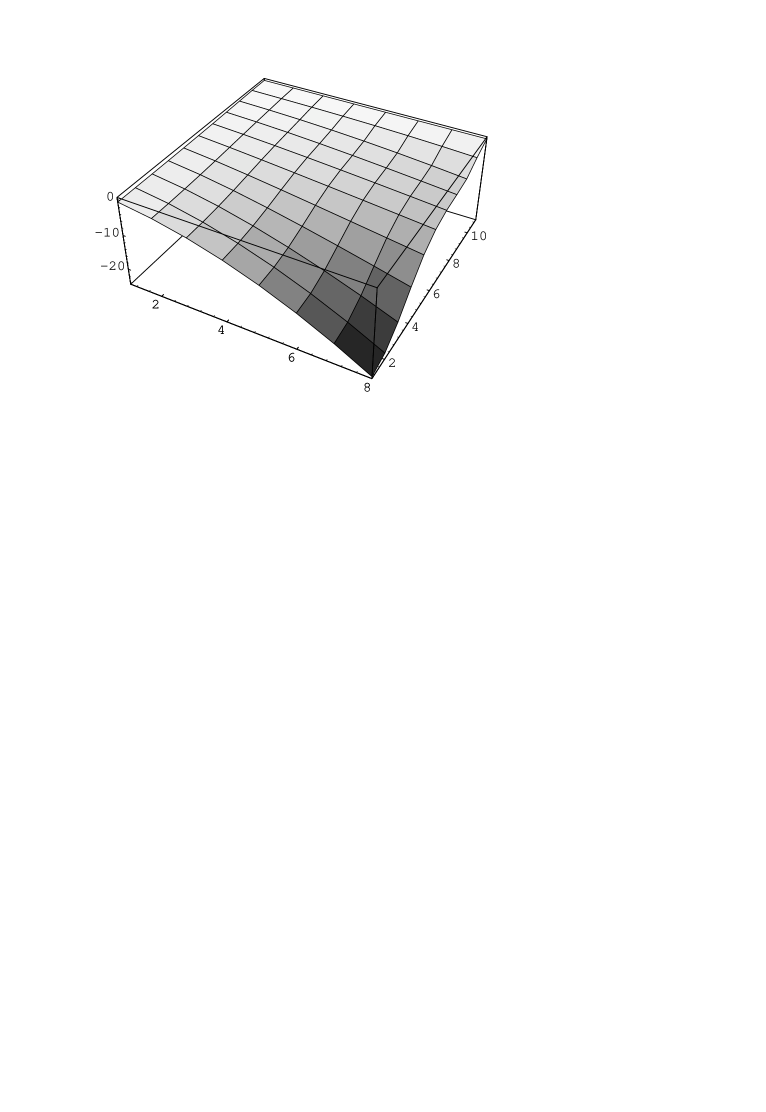
Figure 5: $\Omega^{k}$ versus for $k$ going from $2$ to $9$. The axis labeled with $2$, $4$, $6$ and $8$, on the left, is $k-1$. The axis with labels going up to $10$, on the right, is the $\theta$ axis. $\theta$ goes from $0$ to $\pi$. $\theta=0$ coincides with the tick $1$, $\theta=\frac{\pi}{2}$ with the tick $6$ and $\theta=\pi$ with the tick $11$. $q=1$ on the left limit of the axis (ferromagnet), $q=0$ (spin glass) in the center and $q=-1$ (fully frustrated model) on the right edge of the axis. The vertical axis is for $\Omega^{k}$. Decreasing values of $\Omega^{k}$ are drawn with darker coloring.

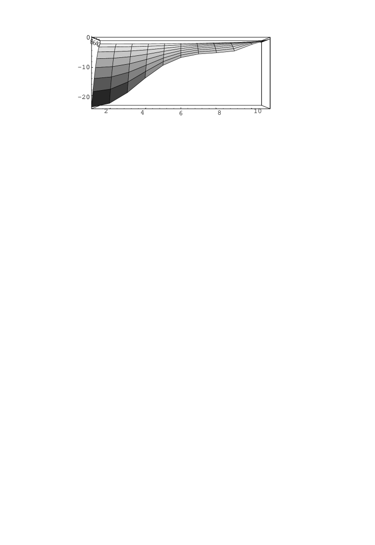
Figure 6: As in fig. (5), but from a different point of view. Here the $x$ axis is $\theta$ ($0$ on the left and $\pi$ on the right), the $y$ axis is $\Omega$ and the $k$ axis goes beyond the page. We sit on the side of high $k$ values.

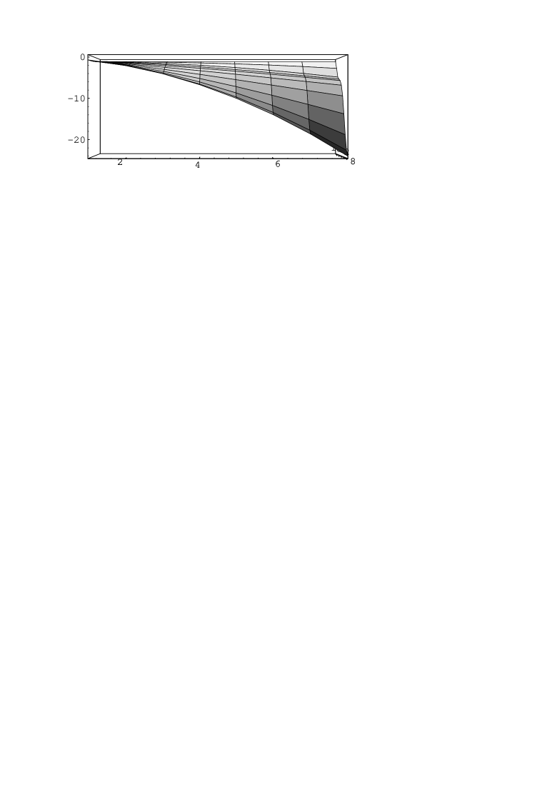
Figure 7: As in fig. (5), but from a different point of view. Here the $x$ axis is $k$ ($2$ on the left and $9$ on the right), the $y$ axis is $\Omega$ and the $\theta$ axis goes beyond the page. We sit on the side of $\theta\simeq 0$ values.

We plot the $\Omega$ surface as a function of $k$ and $\theta$ from different viewpoints in figures (5-7). It is interesting to note that moving away from $\theta=\frac{\pi}{2}$ in the direction of the fully frustrated model, i.e. increasing $\theta$, $\Omega$ changes quite smoothly. On the contrary when $\theta$ becomes smaller than $\theta=\frac{\pi}{2}$ the change is far more abrupt. This is coherent with what we find from fig. (3) where for negative values of $q$ the system does not change much, and fig. (4) where $q>0$ the system undergoes a strong quantitative change around $q=\frac{1}{2}$. This point is where in figures (5-7) we can find a maximal change of $\Omega$ as a function of $q$. The plateau that one sees when moving to the right of fig. (6) can be seen in perspective in fig. (7).

We have also checked that the results are in reasonable agreement with the ansatz

$$\frac{R^{k}_{D}}{R^{k-1}_{D}}=a+\frac{b(\frac{k}{D})}{D}\ ,$$ (55)

where the function $b(w)$ does not seem to have a fast divergence for large values of $w$. Apparently the limit $D\to\infty$ is smooth.

5 The Low Temperature Region

In the former section we have discussed the high $T$ region of the deterministic model with complex frustration. We have shown that the Monte Carlo data reproduce well (but for the case of high, positive $q$, where finite size effects are dramatic) the series obtained by computing the Green functions of the $q$-deformed harmonic oscillator. Together with the results of ([3]) and the Appendix of this note that makes the status of the high $T$ phase clear. We also know that in the high $T$ phase the model with quenched disorder coincides by construction with the deterministic model, but we will see that better in the following.

In order to get information about the low $T$ phase we have to use the random model, which we have defined in eqs. (25,26). We will use replica theory to solve it both in the high $T$ phase (where we will find again the same high $T$ series) and in the low $T$ phase. We will try to understand how much the replica formulation of the system is connected to the Monte Carlo data we will get directly from the deterministic model with complex frustration.

Let us solve the random model by using the techniques introduced in [1, 2]. The computation follows quite closely the one of [1, 2], and we will give here only the main details. One introduces $n$ replicas, where $n$ has to be sent to zero at the end of the computation. The $n$-dependent free energy is given by

$$f^{(n)}(\beta)\equiv-\lim_{N\to\infty}{1\over\beta N}\frac{\overline{Z_{U}^{n}}-1}{n}\ ,$$ (56)

where the bar denotes the average over the random couplings and the replicated partition function $Z_{U}^{n}$ depends over the noise and can be written as

$$Z_{U}^{n}\equiv\int[d\sigma]e^{-\beta\sum_{a=1}^{n}H_{U}^{a}}\ .$$ (57)

The integration over the unitary group can be done explicitly. After some algebra one finds that one has to evaluate the stationary points of the following free energy:

$$A[Q,\Lambda]=-\mbox{Tr}G(\beta Q)+\mbox{Tr}(\Lambda Q)-F(\Lambda)\ ,$$ (58)

where $Q$ and $\Lambda$ are $n\times n$ matrices, the function $G$ is related to the one defined in eq. (33) by

$${dG\over dz}\equiv E(z)\ ,$$ (59)

and

$$F(\Lambda)\equiv\ln\int d[\sigma]\exp(\sum_{a,b}\Lambda_{a,b}\sigma^{a}\sigma^{b})\ .$$ (60)

In the high temperature phase the off-diagonal terms of the two matrices $Q$ and $\Lambda$ are zero. If we set

$$Q_{a,b} = \delta_{a,b}\ q\ ,$$

$$\Lambda_{a,b} = \delta_{a,b}\ \lambda\ ,$$ (61)

we find that the stationary equations imply that

$$q=1\ \mbox{and}\ \lambda=E(\beta)\ .$$ (62)

We finally find that in the high temperature phase

$${\partial F\over\partial\beta}=E(\beta)\ ,$$ (63)

where $E(\beta)$ is the function defined in (59). In this way we have derived again the equivalence of the model with quenched disorder and the deterministic model with complex frustration in the high temperature phase.

In the low temperature region the off-diagonal terms of the two matrices are non-zero. If we assume that replica symmetry is unbroken, we have that the off-diagonal terms are given by

$$Q_{a,b} = q\ ,$$

$$\Lambda_{a,b} = \lambda\ .$$ (64)

In this way we find that we have to minimize the free energy

$$G(\beta(1-q))+\beta qE(\beta(1-q))-\lambda q+f(\lambda)\ ,$$ (65)

where the function $f$ is given by

$$\ln\bigl{(}\int dh\exp(-h^{2}/2)\bigr{)}\ln\bigl{(}\int d\sigma_{r}d\sigma_{i}\delta(\sigma_{r}^{2}+\sigma_{i}^{2}-1)\exp(-\lambda^{\frac{1}{2}}h\sigma_{r})\bigr{)}\ .$$ (66)

The energy turns out to be

$$E(\beta)=G^{\prime}(\beta(1-q))-\beta q(1-q)G^{\prime\prime}(\beta(1-q))\ .$$ (67)

By deriving this expression and evaluating it for $\beta=\beta_{c}$ we find that

$$C_{V}(\beta_{c}^{+})=C_{V}(\beta_{c}^{-})=1\ .$$ (68)

The critical temperature can also be determined through the relation

$$\beta_{c}^{2}G^{\prime\prime}(\beta_{c})=1\ .$$ (69)

One also finds that at zero temperature

$$C_{V}(\infty)=\frac{1}{2}\ ,$$ (70)

in agreement with the equipartition theorem.

The equations which determine the minimum of such free energy can be solved numerically.

We will show and discuss their solution in next section, for different $q$ values, together with the Monte Carlo results in the low $T$ phase.

We expect the unbroken replica solution to give rather accurate values for the free energy. In the SK model the error over the correct, replica broken result is smaller than $3\%$, and it is likely to be even smaller in the present case. It is interesting to note that the replica symmetric solution normally gives a lower bound to the true free energy and to the true internal energy of the system. Our numerical simulations show that when we compare numerical simulations of the deterministic model to the replica symmetric solution of the disordered model in the cold phase this is not always the case in our system, pointing to a non complete coincidence of the two models.

6 Computer Simulations

We will describe here our numerical simulations of the model with complex frustration and no quenched disorder (but for the small one needed for constructing the antisymmetric tensor ${\cal S}$), defined with the couplings of eq. (12), and compare them with the analytic solution of the model with quenched disorder that we have discussed in the previous section. Here we will mainly focus on the low $T$ phase.

We have simulated systems with $D$ going from $3$ to $15$ or $16$, i.e. containing from $8$ to $32768$ or $65536$ sites. We have been starting from all fields set to $1$ at high $T$, and decreased the temperature in small steps. A typical pattern has been starting from $T=4.05$, and decreasing it down with $80$ steps of $\Delta T=.05$ (but for some runs we only used $40$ steps and a lower starting point). At each next $T$ we have been continuing from the last configuration obtained at $T+\Delta T$. At each $T$ value we have used $500$ full sweeps of the system to obtain an acceptance value of the Monte Carlo procedure of $50\%$ (by tuning the angular increment we would propose for updating the field phase in a given site). After that we have used $1250$ full sweeps to thermalize the system, and $5000$ full sweeps to measure the internal energy. We have ran some longer simulations to check we have indeed reached thermal equilibrium, and it seems to be the case. We believe that the statistical error on our data points is always smaller than the symbols we use to plot them. We have always only used in the final plots the data from a single realization of the antisymmetric tensor ${\cal S}$ (even if we have checked the size of typical fluctuations by simulating more than one ${\cal S}$ set, and the induced uncertainty turned out to be not very large, but detectable).

As a first check we have verified we could reproduce the results obtained in [4] for the fully frustrated model.

A second preliminary question was concerning the equality of the traces of the $n$-th powers of the coupling matrix and the expectation values of the operators which appear in the formalism of the $q$-deformed harmonic oscillator. This is a point which has been proven in ([3]) and in this note, and verifying it was meant to constitute both a check of our codes and of our theorems. So given the couplings we have selected, according to eq. (12) and to a random choice of the ${\cal S}$ (over which in this case we have averaged) we have verified that

$$2^{-D}\mbox{Tr}(\Delta_{q}^{n})=\langle 0|{\cal X}^{n}_{q}|0\rangle\ .$$ (71)

In this case we have kept the statistical error (given in this case by the distribution of the ${\cal S}$, and not by a Monte Carlo: there is no Monte Carlo here!) under careful control. All momenta up to $n=8$ coincide with the $q$-deformed result with a better precision than $10^{-3}$. Our best fits give the right answer, with a $\chi^{2}$ of order one per degree of freedom. So, this check has been positive, and it is an important check of the equivalence of the model with complex frustration and the random model in the high $T$ phase.

We come now to the main point of our investigation, i.e. the low $T$ phase. Here we will compare the analytic solution of the random model (25) with the numerical simulation of the deterministic model. We will see that the data are indicative of a strong similarity, but not of a complete equivalence of the two models.

Figure 8: Energy of the $q=0$ model versus $T$. Here we are looking at both phases (the critical point is at $T_{c}=1$). See the text for the explanation of the different symbols. The point where the dashed line becomes continuous is here and in the following figures the critical point.

In fig. (8) we plot the energy of the $q=0$ model versus $T$, in both phases (the critical point is at $T_{c}=1$). The point where the dashed line becomes continuous is here and in the following figures the critical point. We plot the analytic result from the high $T$ expansion with a dashed line, while the result obtained by minimizing eq. (65) is plotted with a continuous line, for $T<T_{c}$. Here we include the data from all our simulations. The fancy starred dots, lying at the top, are from $D=3$. Crosses are for intermediate values of $D$ (lower points for higher $D$ values). For the four higher values of $D$ (in this case $D=13$, $14$, $15$ and $16$) we change symbol again, and we use respectively empty triangles, empty squares, filled triangles and filled squares.

The agreement of Monte Carlo data for the deterministic model and replica symmetric solution of the random model is quite good also in the broken phase, for $T<T_{c}$. We expect that the solution with broken replica symmetry will have an energy slightly higher than the unbroken one (as we already said, in the general case the replica symmetric energy is a lower bound to the true energy of the physical system). Very small residual finite size effect, and this small energy drift to the the breaking of replica symmetry should explain the small discrepancy between the numerical data and the analytic curve. So in the case of the $q=0$ model things seem to go smoothly.

When moving on the side of negative $q$ values things do not change much, and if there is a discrepancy it is very small. This is completely coherent with the discussion of the behavior of the coefficients of the high $T$ expansion of former section.

Figure 9: As in fig. (8), but for $q=-.233$.

Figure 10: As in fig. (8), but the specific heat $C_{V}$ for $q=-.233$. For sake of graphical clarity here we only use crosses for $D=12$ data and filled squares for $D=16$, and we join the data points with dotted lines.

In fig. (9) the results for $q=-.233$ (where the angle is already different of a $15\%$ from $\theta=\frac{\pi}{2}$). The agreement of our data with the analytic solution are still quite good. Fig. (8) and fig. (9) are on the same scale (as it will be for all the following energy plots). That allows the reader to appreciate that indeed the two energy plots are quite different among them. To show even better that things are basically working in this regime of negative $q$ values we plot in fig. (10) the specific heat for $q=-.233$. The small gap in the analytic curve close to the maximum is because we stopped early our numerical evaluation of the high $T$ series. We cannot detect here any clear discrepancy.

Figure 11: As in fig. (8), but for $q=-.5$.

Figure 12: As in fig. (10), but $q=-.5$.

We show in figures (11) and (12) that even at very high negative values of $q$ (i.e. at least down to $q=-0.5$) our replica solution of the model with quenched disorder gives a very accurate description of the behavior of the deterministic model with complex frustration in the low $T$ phase. Even the specific heat very close to the critical point is reconstructed with good accuracy.

Figure 13: As in fig. (8), but for $q=.078$. Here the dashed straight line is the result one would get for the spherical model, where the energy becomes linear in $T$ below the critical point.

Figure 14: As in fig. (10), but $q=.078$.

The situation is different on the side of $\theta<\frac{\pi}{2}$, i.e. for positive values of $q$. At low positive $q$ there are again no dramatic problems, and if the two models differ they do differ only in a very minor way. In fig. (13) we add a dashed straight line, from $T_{c}$ down to $T=0$, to give the result one would obtain for the spherical model [13], where the energy becomes linear in $T$ below the critical point. In fig. (14) we plot again the specific heat. If there is a discrepancy it small, even if we want already to notice the small bump just under $T_{c}$, which makes the Monte Carlo data slightly different from the disordered model result. This effect was not there for negative $q$ values, and it is not clear here if it is due to a true difference or if it is connected to a finite size effect.

Figure 15: As in fig. (8), but for $q=.233$.

Figure 16: As in fig. (10), but $q=.233$.

The situation becomes more clear (in a negative sense) when we increase $q$ of a not huge amount. We give in figures (15) and (16) the results for $q=.233$, and here there is a clear discrepancy, which is difficult to justify by means of finite size effects. Indeed here the energy of the Monte Carlo simulations at low $T$ is, already for $D=16$ lower than the analytic result one gets for the spherical random model in the infinite volume limit. Since the energy is decreasing with $D$, and we expect the energy of the spherical model to be a lower bound at all $T$ to our XY case, that seems to show that in this case the two models do indeed differ, even if only of a small amount. In order to explain this effect one would have to assume that the sign of the corrections changes with the dimensionality, and that the energy will go up again for $D$ large enough. This is not impossible, but not so plausible, and we have no numerical indications for such an effect to be taking place. The specific heat picture (16) is even more self-explanatory than the energy, since it is quite difficult to believe that the big bump of the Monte Carlo data will be reabsorbed in the $D\to\infty$ limit.

In conclusion, it seems that for $q<0$ and even for small $q$ positive values the replica theory describes the deterministic model with very high accuracy. On the contrary for $q>0$ not so small there is a clear, even if quite small discrepancy between the two models.

Appendix

In this short appendix we will fill a gap in the proof of equation (36). We only sketch the main steps of the proof, which is absolutely inelegant. It is quite likely that a more elegant proof, e.g. based on the braid group, do exist, but we have not found it.

In [3] it was proved that

$$G_{k}^{(q)}\equiv\int d\lambda\ \rho_{\Delta}(\lambda)\ \lambda^{n}=\sum_{n=0,\infty}{\cal N}(k,n)q^{n}\ ,$$ (72)

where ${\cal N}(k,n)$ is the number of ways in which one can connect piecewise $k$ points on a circle, with $n$ intersections.

In order to compute ${\cal N}(k,n)$ it may convenient to consider the quantity ${\cal N}(k,n,m)$, i.e. the number of ways in which $k+1$ points on the circle may be connected in such a way that a line starts from each of the first $k$ points and $m$ lines arrive in the last $k+1$-th point, the total number of intersection being $n$. It is evident that

$${\cal N}(k,n)={\cal N}(k,n,0)\ .$$ (73)

A simple pictorial argument can be used to prove that

$${\cal N}(k+1,n,m)={\cal N}(k,n,m-1)+\sum_{j=0,m}{\cal N}(k,n-j,m+1)\ .$$ (74)

We can now check that this relation is satisfied if we set

$$\sum_{n=0,\infty}{\cal N}(k,n,m)q^{n}\equiv G_{k}^{(q)}(m)=\langle m|Y^{k}|0\rangle$$ (75)

where the $|n\rangle$ (for $n=0,\infty$) form a basis in an Hilbert space,

$$Y\equiv A+A^{\dagger}\ ,$$ (76)

and

$$A|n\rangle = |n-1\rangle\ \mbox{for}\ n\not=0\ ,$$

$$A|0\rangle = 0\ ,$$ (77)

$$A^{\dagger}|n\rangle = \frac{1-q^{n+1}}{1-q}|n+1\rangle\ .$$

The operator $X$ in eq. (36) and $Y$ are related by the simple transformation $X=MYM^{-1}$, where the operator $M$ is diagonal in the basis we have used. We finally find that

$$G_{k}^{(q)}(0)=\langle m|Y^{k}|0\rangle=\langle m|X^{k}|0\rangle\ ,$$ (78)

which is the result announced in [3].

References

- [1] E. Marinari, G. Parisi and F. Ritort, hep-th/9405148, J. Phys. A: Math. Gen. 27 (1994) 7615.
- [2] E. Marinari, G. Parisi and F. Ritort, cond-mat/9406074, J. Phys. A: Math. Gen. 27 (1994) 7647.
- [3] G. Parisi, cond-mat/9410088, J. Phys. A: Math. Gen. 27 (1994) 7555.
- [4] E. Marinari, G. Parisi and F. Ritort, cond-mat/9410089, J. Phys. A: Math. Gen. 28 (1995) 327.
- [5] G. Parisi, Field Theory, Disorder and Simulations (World Scientific, Singapore 1992).
- [6] D. A. Huse and H. S. Seung, Phys. Rev. B42 (1990) 1059.
- [7] J. D. Reger, T. A. Tokuyasu, A. P. Young and M. P. A. Fisher, Phys. Rev. B 44 (1991) 7147.
- [8] M. J. P. Gingras, Phys. Rev. B45 (1992) 7547.
- [9] G. Parisi, Statistical Field Theory (Addison Wesley, Redwood City, CA, USA 1988).
- [10] S. Kirkpatrick and D. Sherrington, Phys. Rev. B 17 (1978) 4384.
- [11] E. Brezin, C. Itzykson, G. Parisi and J. B. Zuber, Comm. Math. Phys. 59 (1978) 35.
- [12] J. P. Bouchaud and M. Mezard, J. Physique I (Paris) 4 (1994) 1109.
- [13] J. M. Kosterlitz, D. J. Thouless and R. C. Jones, Phys. Rev. Lett. 36 (1976) 1217.