Singularities in the Fermi liquid description of a partially filled Landau level and the energy gaps of fractional quantum Hall states

Abstract

We consider a two dimensional electron system in an external magnetic field at and near an even denominator Landau level filling fraction. Using a fermionic Chern–Simons approach we study the description of the system’s low energy excitations within an extension of Landau’s Fermi liquid theory. We calculate perturbatively the effective mass and the quasi–particle interaction function characterizing this description. We find that at an even denominator filling fraction the fermion’s effective mass diverges logarithmically at the Fermi level, and argue that this divergence allows for an exact calculation of the energy gaps of the fractional quantized Hall states asymptotically approaching these filling fractions. We find that the quasi–particle interaction function approaches a delta function. This singular behavior leads to a cancelation of the diverging effective mass from the long wavelength low frequency linear response functions at even denominator filling fractions.

I Introduction

The Fermionic Chern–Simons theory has been extensively used in the last few years to describe the physics of a two dimensional electron gas in a partially filled Landau level [2] – [7]. In that theory, the problem of electrostatically interacting electrons in a strong magnetic field is converted, using an exact transformation, to a problem of electrostatically interacting ”transformed fermions” which also interact with a Chern–Simons gauge field.

Being still unsolvable, the transformed fermion problem is studied by approximations. The simplest approximation, mean field theory, already gives interesting physical results. For example, it predicts the existence of stable quantized Hall states at filling fractions of the form $\frac{p}{\tilde{\phi}p+1}$, where $p$ is an arbitrary integer, and $\tilde{\phi}$ is an even positive integer, equal to the number of quanta of Chern–Simons flux attached to each fermion. As was first noted by Jain [8], filling fractions of the above form, with $\tilde{\phi}=2$, are the most prominent fractional Hall states seen in the lowest Landau level. (Jain’s ”composite fermions” may be regarded as equivalent to the transformed fermions, projected onto the lowest electronic Landau level.) By contrast, at the even denominator fractions $1/\tilde{\phi}$, the fermion Chern–Simons mean field theory predicts a Fermi–liquid state, with no energy gap and no quantized Hall effect [2][4].

For a description of the excitation spectrum and of other quantities of interest, it is of course necessary to go beyond mean field theory. Specifically, it is necessary to consider, using perturbation theory, the effects of fluctuations in the Chern–Simons field and of the two body interaction, effects which are omitted from mean field theory. Consequences of these perturbations were explored at some length by Halperin, Lee and Read (HLR)[2] for the Fermi liquid state at $\nu=1/\tilde{\phi}$, and also to some degree for other nearby filling fractions.

An interesting result of the HLR analysis was the prediction that at $\nu=1/\tilde{\phi}$ the effective mass $m^{*}$ of the transformed fermions diverges for quasi–particles at the Fermi energy. For the physically relevant case of Coulomb interaction between the electrons, this divergence was found to be quite weak, i.e., logarithmic in $\omega$, the energy relative to the Fermi energy. For short range electron–electron interaction HLR found a stronger divergence $m^{*}\sim\omega^{-1/3}$, while for a longer range interaction the effective mass remains finite as $\omega\rightarrow 0$.

The HLR results were based on an examination of the leading diagrams in the perturbation expansion for small $\tilde{\phi}$, supplemented by heuristic arguments that the leading singularity might not be affected by higher orders in perturbation theory. Consequently, it is of interest to see whether these arguments can be made more convincing, or whether by contrast results contradictory to HLR may be obtained. Interest in these questions has been stimulated by the fact that similar effective mass divergences are found in other models in which fermions interact strongly with a fluctuating gauge field, including models that have been advanced in the context of high $T_{c}$ superconductivity [5]–[12].

Assuming that the effective mass divergence predicted by HLR is indeed correct, one may ask what physically measurable quantities might reflect it. According to HLR, the renormalized mass should $not$ show up in the long wavelength density and current response functions at zero temperature, for $\omega/q\rightarrow 0$. This observation was confirmed, more recently, by analyses using a variety of theoretical techniques, including renormalization group methods [9][10], bosonization [5] and diagrammatic analyses[6]. Moreover, Kim et.al.[6], using an approximation that takes into account the leading divergent contribution to $m^{*}$, have shown that there is no corresponding singularity in the density response function in the limit of low frequencies and long wavelengths, for any value of $\omega/q$. Within their approximation, the density response function looks just like the one obtained in the random phase approximation of a Fermi gas with the bare mass $m$. The diverging effective mass may be expected to show up in the temperature dependence of the specific heat at low temperatures; however, a contribution from the low frequency density relaxation collective mode could lead to the same anomalous temperature dependence as the quasiparticle contribution.

As noted by HLR, a more definitive manifestation of the diverging $m^{*}$ should come from the behavior of the energy gap at quantized Hall steps for $\nu=\frac{p}{\tilde{\phi}p+1}$, for large values of $p$. Specifically, one might expect the energy gap $E_{g}(\nu)$ to be

$$E_{g}(\nu)=\frac{\hbar e|\Delta B|}{m^{*}(\nu)c}$$ (1)

where $m^{*}(\nu)$ is the effective mass calculated self–consistently at an energy $E_{g}(\nu)$, and $\Delta B\equiv B-2\pi\tilde{\phi}{n}$ is the deviation of the magnetic field from its value at $\nu=1/\tilde{\phi}$. Here we denote the average density of electrons by ${n}$, and we use units where $\hbar=\frac{e}{c}=1$. Until now, however, the conjecture (1) has not been checked by any explicit calculation.

In this paper we study both the even denominator state and the way it is approached when the filling fraction is slightly away from it. We study the properties of the Fermi liquid formed at an even denominator filling fraction (e.g., $1/2$), namely, the effective mass and the quasi–particle interaction function. We review the perturbative calculation leading to the divergence of the effective mass, and find that for the Coulomb case, as $\omega\rightarrow 0$, the leading term in the effective mass is,

$$m^{*}(\omega)=\frac{\tilde{\phi}^{2}}{2\pi}\frac{\epsilon k_{F}}{e^{2}}|\ln{\omega}|$$ (2)

where $\epsilon$ is the background dielectric constant, $\omega$ is the distance from the Fermi energy and the Fermi wavevector $k_{F}$ is related to the electron density by $k_{F}=(4\pi n)^{1/2}$. We then argue that Eq. (2) is the exact leading term in the limit $\omega\rightarrow 0$. This statement is based on the use of Ward’s identity to account for the renormalization of the vertices in the diagram leading to the divergence of $m^{*}$. We directly calculate the energy gap at a filling factor of the form $\nu=\frac{p}{\tilde{\phi}p+1}$, and confirm the conjecture (1). Thus, for large $p$, the energy gap we obtain is,

$$E_{g}\approx\frac{\pi\sqrt{2}}{\tilde{\phi}^{3/2}}\frac{e^{2}}{\epsilon l_{H}}\frac{1}{(\tilde{\phi}p+1)\ln{(\tilde{\phi}p+1)}}$$ (3)

where $l_{H}\equiv\sqrt{\frac{\hbar c}{eB}}$ is the magnetic length. Following our discussion of the effective mass, we argue that our expression for the energy gap, Eq. (3), is exact in the $p\rightarrow\infty$ limit [14]. In our study of the Landau quasi–particle interaction function at $\nu={1/\tilde{\phi}}$ we find that it includes a singular contribution that is just of the form necessary to explain the results of Kim et.al. [6], i.e., of the form needed to cancel the effect of a diverging effective mass on the zero temperature long wavelength low frequency linear response function. The expression we find for the Landau quasi–particle interaction function is, however, not exact. In particular, our approximation does not properly account for the effects of short wavelength and high frequency fluctuations. These fluctuations are particularly important in the limit where the electron’s bare mass is vanishingly small, so that the cyclotron energy becomes infinite and the actual electron states are projected onto the lowest Landau level; our approximation incorrectly predicts the magnitude of the Landau interaction function in this limit. The short wavelength and high frequency fluctuations are not important for the effective mass $m^{*}$ and the energy gaps at $p\rightarrow\infty$, because these quantities are determined by infra–red divergences in the self energy.

Combining our analysis of the effective mass and the quasi–particle interaction function, we study the behavior of the chemical potential $\mu$ of the composite fermions as the density ${n}$ is varied and $\Delta B$ is kept fixed. We find that the chemical potential jumps discontinuously whenever the density corresponds to an integer fermionic filling factor $p$. The magnitude of the jump is the energy gap corresponding to the fractional quantum Hall state at $\nu=\frac{p}{\tilde{\phi}p+1}$. As emphasized above, it reflects the divergence of $m^{*}$. However, we also find that the chemical potential varies continuously during the course of a population of a fermions’ Landau level. This variation is such that the overall slope of $\mu({n})$ is independent of the divergent contribution to $m^{*}$ (See Fig. (5)).

In our perturbative study of the Fermion’s effective mass, energy gaps and Landau interaction function, we use the RPA expression for the gauge field propagator. This use is then justified by our results. The singularities we study result from the long wavelength low frequency behavior of the gauge propagator. The latter are determined by the long wavelength low frequency limit of the fermion’s polarization functions (the fermions irreducible polarization bubble). As we show, and as was shown before by several authors [6][7][10], in that limit, the fermions’ irreducible polarization functions are not renormalized by gauge field fluctuations.

The outline of the paper is as follows: in Section (2) we construct a general framework for the discussion of the Fermi liquid formed by the composite fermions. In Section (3) we calculate perturbatively the parameters characterizing this Fermi liquid, and we discuss the regime of validity of the perturbative approach. In Section (4) we examine the linear response function resulting from the parameters obtained in Sec. (3). In Section (5) we calculate the energy gaps for large $p$, and analyze the dependence of the chemical potential on the density for fixed $\Delta B$. In Section (6) we comment on the effect of the coupling of the fermions to longitudinal gauge fluctuations. We conclude with a summary.

Several details of the analysis of Section (3) are given in Appendices A and B.

II General description of the Fermi liquid of the composite fermions

In this section we define the model to be considered, and we give a general description of the Fermi liquid formed at even denominator filling fractions. We consider electrons in a two dimensional electron gas, subject to a magnetic field $B$. The electrons interact via a Coulomb interaction, $V({\bf r}-{\bf r^{\prime}})=\frac{e^{2}}{\epsilon|{\bf r}-{\bf r^{\prime}}|}$. Using a singular gauge transformation, the problem is mapped onto that of fermions subject to a magnetic field $\Delta B=B-2\pi{n}\tilde{\phi}$. (In our system of units, where $\hbar=\frac{e}{c}=1$, the flux quantum is $2\pi$.) In the case we discuss in this section, the electronic filling factor is $1/\tilde{\phi}$, and then $\Delta B=0$ and the fermionic filling factor, $p$, is infinite. In section (5) we discuss the case of finite $\Delta B$ and $p$. Generally, the fermions’ Hamiltonian is

$$\begin{array}[]{ll}H=&{1\over{2m}}\int d^{2}r\Psi^{+}({\bf r})[-i{\bf\nabla}+\Delta{\bf{A}}({\bf r})-{\bf a}({\bf r})]^{2}\Psi({\bf r})\\ \\ &+{1\over 2}\int d^{2}r\int d^{2}r^{\prime}[\Psi^{+}({\bf r})\Psi({\bf r})-{n}]V({\bf r}-{\bf r^{\prime}})[\Psi^{+}({\bf r^{\prime}})\Psi({\bf r^{\prime}})-{n}]\\ \\ \end{array}$$ (4)

supplemented by the gauge condition ${\bf\nabla}\cdot{\bf a}=0$ and by the constraint ${\bf\nabla}\times{\bf a}({\bf r})=2\pi\tilde{\phi}[\Psi^{+}({\bf r})\Psi({\bf r})-{n}]$, where ${n}$ is the average electron density. In Eq. (4) $\Delta{\bf A}({\bf r})=\frac{1}{2}\Delta B{\hat{z}}\times{\bf r}$. The constraint may be used to write the electrostatic term as ${1\over{2(2\pi\tilde{\phi})^{2}}}\int d^{2}r\int d^{2}r^{\prime}[{\bf\nabla}\times{\bf a}({\bf r})]V({\bf r}-{\bf r^{\prime}})[{\bf\nabla}\times{\bf a}({\bf r^{\prime}})]$. The fermion’s interaction with the transverse gauge field is then of the form $-{\bf J}\cdot{\bf a}-{1\over{2m}}\rho{\bf a}^{2}$ where ${\bf J},\rho$ are the fermions’ current and density. The Fermi wave-vector of the fermions is $k_{F}=\sqrt{4\pi{n}}$.

At the mean field approximation, the Chern–Simons gauge field ${\bf a}$ is replaced by its average value, and thus its interaction with the fermions is neglected. In this section we attempt to describe the effect of these interactions on the fermions within an extension of Landau’s Fermi liquid theory. Landau’s theory describes the low energy excitations of the system in terms of the occupation number function $n({\bf k})$ [16]–[18]. This function signifies the difference between the occupation number of the state $\bf k$ at the excited state and the corresponding number at the ground state. The energy density corresponding to a given function $n({\bf k})$ is

$${\cal E}\Big{(}n({\bf k})\Big{)}={{\int\frac{d^{2}k}{(2\pi)^{2}}}}\epsilon_{\bf k}n({\bf k})+{1\over 2}{{\int\frac{d^{2}k}{(2\pi)^{2}}}}{{\int\frac{d^{2}k^{\prime}}{(2\pi)^{2}}}}f({\bf k,k^{\prime}})n({\bf k})n({\bf k^{\prime}})$$ (5)

where $\epsilon_{\bf k}=\frac{k^{2}}{2m^{*}}$ is the kinetic energy of a quasi–particle near the Fermi level, $m^{*}$ is its effective mass, and $f({\bf k},{\bf k^{\prime}})$ is the Landau interaction function. Note that in the presence of a non–zero vector potential, $\bf k$ is the dynamical momentum, and not the canonical one.

The parameters $m^{*},f$ include the entire effect of the interaction near the Fermi level in the case of a neutral fluid such as ${}^{3}{\rm He}$ in its normal state, but they conventionally leave out the direct, Hartree, part of the interaction in the case of electrons in a metal. The difference between the two cases is in the range of the interactions being short for Helium atoms and long for electrons in metals. As developed in Silin’s extension of Landau’s theory [18], the effect of long range interactions is taken into account when linear response functions are calculated, by making a distinction between the externally applied driving force and total driving force. In the problem we consider, the Chern–Simons interaction of the fermions with the gauge field is long ranged. Consequently, the direct Hartree part of both that interaction and the electrostatic one should be separated from the rest. Thus, our construction of the Fermi liquid picture for the composite fermions starts by defining the energy functional (5) excluding the contribution of the direct Hartree part of both interactions. Then, we use the equation of motion derived from that functional to define and calculate a linear response function of the fermions.

The equation of motion is conveniently written as an integral equation for the function $\nu(\theta)$, defined by $n({\bf k})\equiv\delta(k-k_{F})\nu(\theta)$, where $\theta$ is the angle between $\bf k$ and some reference direction [16]–[18]. The function $\nu(\theta)$ describes the deformation of the Fermi surface in the direction $\theta$. The equation of motion for $\nu(\theta)$ is

$$(\omega-{q}{v_{F}^{*}}\cos{\theta})\nu_{{\bf q},\omega}(\theta)-\frac{1}{(2\pi)^{2}}{q}k_{F}\cos{\theta}\int d\theta^{\prime}f(\theta-\theta^{\prime})\nu_{{\bf q},\omega}(\theta^{\prime})={\bf\hat{k}}\cdot{\bf F}_{{\bf q},\omega}$$ (6)

where the angle $\theta$ is the angle between the vectors ${\bf k}$ and ${\bf q}$; the function $f(\theta-\theta^{\prime})$ is the quasi–particle interaction function $f({\bf k,k^{\prime}})$ for two wave-vectors at the Fermi surface, at angles $\theta,\theta^{\prime}$ relative to $\bf q$; $\bf F$ is the driving force, characterized by a wave–vector $\bf q$ and a frequency $\omega$; and the renormalized Fermi velocity is denoted by $v_{F}^{*}$. Eq. (6) is valid for $q\ll k_{F}$ and $\omega\ll\mu$.

In Landau’s Fermi liquid theory the linear response function is extracted from Eq. (6). This equation relates the deformation function $\nu(\theta)$ to the driving force $\bf F$. In terms of $\nu(\theta)$, the fermions’ density is $\rho_{{\bf q},\omega}=k_{F}\int d\theta\nu_{{\bf q},\omega}(\theta)$ while the current density is ${\bf J}_{{\bf q},\omega}=\int d^{2}k\delta(k-k_{F}){\bf u}_{\bf k}\nu_{{\bf q},\omega}(\frac{\bf k\cdot q}{kq})$, with ${\bf u_{k}}\equiv\frac{\bf k}{m^{*}}+\int d^{2}k^{\prime}f({\bf k},{\bf k^{\prime}})\delta(\epsilon_{\bf k^{\prime}}-\mu)\frac{\bf k^{\prime}}{m^{*}}$. The driving force can be expressed in terms of derivatives of a three–vector potential $A_{\nu}$, as ${\bf F}_{{\bf q},\omega}=-i\omega{\bf A}_{{\bf q},\omega}+i{\bf q}A_{0,{\bf q},\omega}$. Thus, by means of Eq. (6), the current vector $J_{\mu}$ can be related to the vector potential $A_{\nu}$ by $J_{\mu}=\Pi_{\mu\nu}A_{\nu}$, and the linear response function $\Pi_{\mu\nu}$ can be calculated. Generally, the linear response function is a matrix relating the current–density three–vector $J_{\mu}$ to the three–vector potential $A_{\nu}$. Since the three–vector $J_{\mu}$ is constrained by the conservation of charge and the three–vector $A_{\nu}$ is constrained by a gauge condition ${\bf\nabla\cdot A}=0$, the linear response function can in fact be described by a $2\times 2$ matrix $\Pi_{\mu\nu}({\bf q},\omega)$, with the two indices taking the values $0$ (for the time component), and $1$ (for the transverse component).

Now we turn to discuss the effect of the Hartree term. The function $\Pi$ relates the current $J_{\mu}$ to the total vector potential acting on the fermions. This vector potential is composed of an externally applied part and a part induced by the fermion current and density. A fermion current–density vector $J_{\mu}$ induces a vector potential $A^{ind}_{\nu}=V_{\mu\nu}J_{\mu}$ where the matrix $V$ is given by,

$$V=\left(\begin{array}[]{ll}{{2\pi e^{2}}\over{\epsilon q}}&\frac{2\pi i\tilde{\phi}}{q}\\ -\frac{2\pi i\tilde{\phi}}{q}&0\\ \end{array}\right)$$ (7)

The diagonal term is the electrostatic potential induced by a charge density. The off diagonal terms describe the vector potential induced by the fictitious flux tubes attached to the fermions.

We can now define the matrix $K$, relating the current–density vector to the externally applied vector potential $A^{ext}_{\nu}$ by $J_{\mu}=K_{\mu\nu}A^{ext}_{\nu}$. Since $A_{\nu}=A_{\nu}^{ext}+A_{\nu}^{ind}$, $K$ is related to $\Pi$ and $V$ by

$$K^{-1}=V+\Pi^{-1}$$ (8)

Thus, the matrix $K$ describes the response of the system to an externally applied vector potential, including both the Hartree and non–Hartree parts of the interaction. In terms of a diagrammatic expansion, the function $\Pi$ is the fermion–hole proper polarization part (irreducible with respect to a single $V$ line), while the function $K$ is a sum of a geometric series, i.e., of a chain of proper polarization parts connected by single interaction lines $V$ (see Fig. (1)).

The difference between the functions $\Pi$ and $K$ should be particularly stressed in the context of the compressibility. Generally, the compressibility is given by the $\omega=0,q\rightarrow 0$ limit of the density linear response function. Denoting the ground state energy per unit volume by $\epsilon_{0}(n)$ where $n$ is the density of particles, the inverse compressibility is $\frac{1}{\chi}\equiv n^{2}\frac{\partial^{2}\epsilon_{0}}{\partial n^{2}}$ [18]. If the derivatives are taken with the external magnetic field $B$ held fixed, the change in density induces a uniform magnetic field $\Delta B$ on the fermions. The fermions respond to the combination of the driving force and the induced uniform $\Delta B$, and their response is therefore described by the linear response function $K$. The function $\Pi$ describes the case in which a change in the density is accompanied by a change in the external magnetic field $B$, in such a way that $\Delta B$ is kept constant. The two conditions yield two very different compressibilities, as can be seen by analyzing the case of non–interacting electrons around $\nu=1/2$. If the density is changed around $\nu=1/2$ with $B$ being kept constant, $\frac{1}{\chi}=0$. However, if $\Delta B$ is to be kept constant, the variation of the density results in a variation of the cyclotron frequency, and thus a variation of the kinetic energy of the lowest Landau level. Then, $\frac{1}{\chi}=\frac{\pi\tilde{\phi}}{m}$. We come back to this distinction in Sec. (5), where we discuss the gaps in the fractional quantum Hall states.

Another use of Eq. (6) is for the analysis of the excitation modes of the system. The solutions of the equation in the absence of $\bf F$ are poles of $\Pi$. They are characterized by a phase velocity $\omega/q$ and by an eigenfunction $\nu(\theta)$. Those solutions for which $\rho_{{\bf q},\omega}={\bf J}_{{\bf q},\omega}=0$ are unaffected by the matrix $V$. They are poles of $K$ as well. Solutions that do not satisfy these requirements are not poles of $K$. Some insight into the solutions of Eq. (6) in the absence of a driving force is obtained by describing $f(\theta)$ by its Fourier components, the ”Landau parameters”

$$f_{l}\equiv\frac{1}{2\pi}\int_{0}^{2\pi}d\theta f(\theta)e^{il\theta}$$ (9)

In ”well behaved” Fermi liquids, the ratio $m^{*}/m$ is a finite number, and only a small, finite number of Landau parameters are appreciably different from zero. In that case Eq. (6) has a continuum of excitation modes at $\omega<v_{F}^{*}q$, and a small number of discrete states at $\omega>v_{F}^{*}q$. As we show in the next sections, the Fermi liquid we consider does not conform to this description.

To conclude this section, we emphasize again the main points in the Fermi liquid picture we construct for the composite fermions. The energy of an excited state is described by the functional (5). The parameters in this functional, $m^{*}$ and $f$, will be calculated in the next section. The Landau function $f$ does not include the Hartree contribution of either the Coulomb or the Chern–Simons interaction.

The linear response of the system can be described in terms of two types of response functions. The first, $\Pi_{\mu\nu}({\bf q},\omega)$, describes the response of the function to the total driving force, while the second, $K_{\mu\nu}({\bf q},\omega)$, describes the response of the system to the externally applied driving force. In the limit $\omega=0$ and $q\rightarrow 0$, $\Pi$ describes the static compressibility when $\Delta B$ is kept fixed, while $K$ describes the compressibility when $B$ is kept fixed. The poles of the linear response functions can be found, within Fermi liquid theory, by use of the equation of motion for $n({\bf k})$, Eq. (6).

III Perturbative calculation of the Fermi liquid parameters

A Starting Point

In this section we calculate perturbatively the parameters characterizing the Fermi liquid state at $\Delta B=0$, namely $m^{*}$ and $f$. Landau’s theory of the Fermi liquid expresses $m^{*}$ and $f$ in terms of the self energy and the interaction operator of fermions at the Fermi level. The latter, in turn, are expressed in terms of the propagators for the fermions and the gauge field. We start this section by writing the propagators of the fermions and the gauge field. Then, we use these propagators to calculate the self energy, and use the self energy to show that the effective mass diverges. Then, we turn to discuss the Landau function, and pay a special attention to keeping internal consistencies between the approximations used. The Landau function we find turns out to have unique properties, which we discuss in detail.

The fermion propagator in space–time representation is defined, as usual, as

$${\tilde{G}}({\bf r},t;{\bf r^{\prime}},t^{\prime})\equiv-i\langle 0|{\hat{T}}\psi^{+}({\bf r},t)\psi({\bf r^{\prime}},t^{\prime})|0\rangle$$ (10)

where $|0\rangle$ is the ground state, ${\hat{T}}$ is the time ordering operator and the creation and destruction operators are expressed in the Heisenberg picture. The gauge field propagator is defined in a similar way. For the case of $\Delta B=0$, both the Hamiltonian (4) governing the time evolution of the system and its ground state are invariant to space and time translations. Therefore, ${\tilde{G}}$ is a function of ${\bf r-r^{\prime}}$ and $t-t^{\prime}$ only, and it is diagonal in Fourier energy–momentum representation. The same applies also to the gauge field propagator, and, obviously, to the bare propagators.

The bare propagator for the fermions is, for $\Delta B=0$,

$$G_{f}^{(0)}({\bf k},\omega)=\frac{1}{\omega+\mu-{{k^{2}}\over{2m}}+i\eta{\rm sgn}(\omega)}\ \$$ (11)

where $\mu$ is the chemical potential for the transformed fermions, and $\bf k$ is a wavevector.

Since ${\bf\nabla}\cdot{\bf a}=0$ the gauge field propagator is a $2\times 2$ matrix $D_{\mu\nu}$, with $\mu=0$ denoting the time component and $\mu=1$ denoting the transverse spatial component. The gauge field propagator we use in the following calculation is obtained by the random phase approximation (RPA). Its value for $\nu=1/\tilde{\phi}$ ($p=\infty$) was calculated in Ref. [2], and was found to be

$$D({\bf q},\omega)=\left(\begin{array}[]{ll}{m\over{2\pi}}&\ \ -i{q\over{2\pi\tilde{\phi}}}\\ i{q\over{2\pi\tilde{\phi}}}&\ \ i\frac{2{n}}{k_{F}}\frac{\omega}{q}-q^{2}({1\over{12\pi m}}+{{e^{2}}\over{2\pi\tilde{\phi}^{2}\epsilon q}})\end{array}\right)^{-1}$$ (12)

In terms of the self energy of states at the Fermi level the effective mass $m^{*}$ is [15]:

$$m^{*}=m\frac{1-\frac{\partial\Sigma}{\partial\omega}|_{\omega=0}}{1+\frac{\partial\Sigma}{\partial\xi_{k}}|_{k=k_{F}}}$$ (13)

where $\xi_{k}=\frac{k^{2}}{2m}-\mu$.

B Lowest–Order–In–$D$ approximation

1 Fermion Effective Mass

The self energy of the fermions is given, to first order in the gauge field propagator $D$, by the diagram given in Fig. (2a),

$$\Sigma(k,\omega)=i\int\frac{d^{2}k^{\prime}}{(2\pi)^{2}}\int\frac{d\Omega}{2\pi}\frac{1}{m^{2}}\frac{({\bf k}\times{\bf k^{\prime}})^{2}}{|{\bf k}-{\bf k^{\prime}}|^{2}}D(|{\bf k}-{\bf k^{\prime}}|,\omega-\Omega)G_{f}^{0}(k^{\prime},\Omega)$$ (14)

There are two singularities in the evaluation of the integral (14). The first results from the high frequency regime of the longitudinal gauge propagator $D_{00}$. It does not affect the effective mass, and its discussion is therefore deferred to section (6). The second results from the infrared regime of $D_{11}$, and is the source of the logarithmic divergence of the effective mass, as we now turn to discuss. In the long wavelength low frequency limit $D$ is dominated by its diagonal transverse component, given by $D_{11}(q,\omega)\approx[i\frac{2{n}}{k_{F}}\frac{\omega}{q}-q{{e^{2}}\over{2\pi\tilde{\phi}^{2}\epsilon}}]^{-1}$. We focus now on that element of $D$, and neglect all the others. The evaluation of the integrals in (14) is similar to that carried out in studies of the electron–phonon coupling [16]. It is convenient to evaluate $\Sigma(k,\omega)-\Sigma(k,0)$ and to introduce a variable $q=|{\bf k}-{\bf k^{\prime}}|$. Most of the contribution to the $k^{\prime}$ integral comes from $k^{\prime}\approx k_{F}$. From the form of the gauge field propagator we observe that the important contribution to the $q$ integral comes from $q>2\pi\tilde{\phi}\sqrt{\frac{2{n}\epsilon\omega}{e^{2}k_{F}}}$. The integral measure is transformed to

$$\int_{0}^{\infty}k^{\prime}dk^{\prime}\int_{0}^{2\pi}d\theta\longrightarrow 2\int_{0}^{\infty}dk^{\prime}\int_{|k-k^{\prime}|}^{k+k^{\prime}}dq\frac{2k^{\prime}q}{\sqrt{q^{2}-(k-k^{\prime})^{2}}\sqrt{(k+k^{\prime})^{2}-q^{2}}}$$ (15)

It is convenient to consider two regimes. In the first regime $\omega>\frac{e^{2}k_{F}}{2\pi\tilde{\phi}^{2}\epsilon}\frac{(k-k_{F})^{2}}{k_{F}^{2}}$, the integral measure can be approximated by $2\int_{0}^{\infty}dk^{\prime}\int_{0}^{2k_{F}}dq$. Then, the integral over $k^{\prime}$ restricts $\Omega$ to satisfy $0<\Omega<\omega$, and the self energy becomes

$$\Sigma(k,\omega)=\frac{\tilde{\phi}^{2}}{2\pi}\frac{\epsilon k_{F}}{me^{2}}\omega\ln{\left(\frac{4e^{2}k_{F}}{\tilde{\phi}^{2}\epsilon\omega}\right)}+i\frac{\tilde{\phi}^{2}}{4}\frac{\epsilon k_{F}}{me^{2}}\omega$$ (16)

Near the Fermi level the real part of $\Sigma$ is larger than its imaginary part, thus justifying the notion of a quasi–particle. The origin of the logarithmic singularity is the $1\over q$ divergence of $D$ for $\omega=0$. Note that the important contributions to $\Sigma$ come from a limited range of frequencies $0<\Omega<\omega$, but from a large range of wave-vectors $2\pi\tilde{\phi}\sqrt{\frac{2{n}\epsilon\omega}{e^{2}k_{F}}}<q<2k_{F}$. Within the approximation used, $\Sigma$ is independent of $k$. Corrections to that approximation (e.g., to the approximation of the integral’s measure) yield a weak and regular dependence on $k$. Substituting the approximation (16) in Eq. (13) we get a logarithmically diverging effective mass, Eq. (2). Note also that the residue $(1-\frac{\partial\Sigma}{\partial\omega})^{-1}$ vanishes at the Fermi level.

In the second regime $\omega<\frac{e^{2}k_{F}}{2\pi\tilde{\phi}^{2}\epsilon}\frac{(k-k_{F})^{2}}{k_{F}^{2}}$, the integral measure (15) is multiplied by a factor of $q\over{k-k_{F}}$ and the singularity in the self energy is weaker. Near the Fermi surface the mass shell is defined by $\omega\ln{\omega}\propto|k-k_{F}|$. Thus, the first regime determines the quasi–particles dispersion relation and the effective mass is infinite. Later we shall argue that the above conclusions do not change when the set of diagrams included in the approximation for the self energy is extended.

2 Landau Interaction Function

We now turn to discuss the Landau function $f$. For a rotationally invariant system the Landau function $f({\bf k},{\bf k^{\prime}})$ is a function of $\theta$, the angle between the vectors ${\bf k},{\bf k^{\prime}}$ (note that $k\approx k^{\prime}\approx k_{F}$). Standard Fermi liquid theory expresses the Landau function in terms of the Green’s function residue $z$ and the proper part of the interaction operator $\tilde{\Gamma}({\bf k}_{1},\omega_{1};{\bf k}_{2},\omega_{2};{\bf k}_{1}+{\bf q},\omega_{1}+\omega;{\bf k}_{2}-{\bf q},\omega_{2}-\omega)$ as [16],

$$f({\bf k},{\bf k^{\prime}})=z_{k_{F}}^{2}{\rm lim}_{\omega\rightarrow 0}{\tilde{\Gamma}}^{\epsilon}({\bf k},0;{\bf k^{\prime}}0;{\bf k^{\prime}},\omega;{\bf k},-\omega)$$ (17)

where $z_{k_{F}}$ is the Green’s function residue for poles on the Fermi surface, and ${\tilde{\Gamma}}^{\epsilon}({\bf k},\omega;{\bf k^{\prime}}\Omega;{\bf k^{\prime}},\Omega;{\bf k},\omega)\equiv{\rm lim}_{\epsilon\rightarrow 0}{\rm lim}_{q\rightarrow 0}{\tilde{\Gamma}}({\bf k},\omega;{\bf k^{\prime}}\Omega;{\bf k^{\prime}+q},\Omega+\epsilon;{\bf k-q},\omega-\epsilon)$. The full interaction operator ${\Gamma}({\bf k},\omega;{\bf k^{\prime}}\Omega;{\bf k^{\prime}+q},\Omega+\epsilon;{\bf k-q},\omega-\epsilon)$, including both the proper and improper parts, is defined through the two particle Green’s function, in a way described in Fig. (3). The proper part, $\tilde{\Gamma}$, is the sum of all diagrams of $\Gamma$ that are irreducible with respect to cutting a single interaction line, carrying a momentum $q$. The exclusion of the improper diagrams from the Landau function stems from the distinction between the linear response function $\Pi$ and $K$, defined in the previous section. The Landau function determines the linear response function $\Pi$, through Eq. (6). Thus, it should include only diagrams that are ”building blocks” for building the particle–hole proper polarization part (see Fig. (1)). The diagrams excluded from the Landau function are those that serve to build the linear response function $K$. Examples are given in Fig. (2). A comprehensive discussion of the distinction between $\Gamma$ and $\tilde{\Gamma}$ is given in Ref. [18].

For our purpose, we find it convenient to rewrite Eq. (17) in a slightly different form. We define

$$\begin{array}[]{ll}\left\{G^{2}({\bf k},\omega)\right\}_{\epsilon}\equiv{\rm lim}_{\epsilon\rightarrow 0}G_{f}({\bf k},\omega+\epsilon)G_{f}({\bf k},\omega)\\ \\ \left\{G^{2}({\bf k},\omega)\right\}_{\bf q}\equiv{\rm lim}_{{\bf q}\rightarrow 0}G_{f}({\bf k+q},\omega)G_{f}({\bf k},\omega)\end{array}$$ (18)

Since $\left\{G^{2}({\bf k},\omega)\right\}_{\epsilon}-\left\{G^{2}({\bf k},\omega)\right\}_{\bf q}=\frac{2\pi im^{*}z_{k_{F}}^{2}}{k_{F}}\delta(\omega)\delta(k-k_{F})$, [16]–[18], Eq. (17) can be written as

$$f({\bf k},{\bf k^{\prime}})={\rm lim}_{\omega\rightarrow 0}{{-i(2\pi)^{2}}\over{m^{*}(\omega)}}\int\frac{k^{\prime}dk^{\prime}}{(2\pi)^{2}}\int\frac{d\Omega}{2\pi}{\tilde{\Gamma}}^{\epsilon}({\bf k},\omega;{\bf k^{\prime}}\Omega;{\bf k^{\prime}},\Omega;{\bf k},\omega)\left[\{G^{2}({\bf k},\Omega)\}_{\epsilon}-\{G^{2}({\bf k},\Omega)\}_{\bf q}\right]$$ (19)

The extraction of an approximation for the Landau function from an approximation for the interaction operator and the Green’s function residue should be done carefully, since the approximations for $z_{k_{F}}$ and for $m^{*}$ do not result from a systematic expansion in powers of a small parameter. Consistency between the approximations used is established by verifying that they satisfy the symmetries of the problem, namely, gauge invariance and galilean invariance. To be consistent with both symmetries, the approximations used should satisfy Ward’s identities. Gauge invariance dictates the identity [16],

$$\frac{\partial\Sigma}{\partial\omega}=i\int\frac{d^{2}k^{\prime}}{(2\pi)^{2}}\int\frac{d\Omega}{2\pi}{\tilde{\Gamma}}^{\epsilon}({\bf k},\omega;{\bf k^{\prime}}\Omega;{\bf k^{\prime}},\Omega;{\bf k},\omega)G_{f}^{2}({\bf k^{\prime}},\Omega)$$ (20)

(Generally, Ward’s identities relate $\Sigma$ to $\Gamma$, and not to $\tilde{\Gamma}$. However, since here there is no direct contribution to the self energy, the contribution of the improper diagrams of $\Gamma$ to the right hand side of Eq. (20) vanishes). When the self energy is evaluated by Eq. (14), Ward’s identity (20) suggests the approximation of the interaction operator by

$${\tilde{\Gamma}}^{\epsilon}({\bf k},\omega;{\bf k^{\prime}}\Omega;{\bf k^{\prime}},\Omega;{\bf k},\omega)=\frac{1}{m^{2}}\frac{({\bf k}\times{\bf k^{\prime}})^{2}}{|{\bf k}-{\bf k^{\prime}}|^{2}}D(|{\bf k}-{\bf k^{\prime}}|,\omega-\Omega)$$ (21)

and of the Green’s function by $G_{f}=G_{f}^{(0)}$. It can be shown that this approximation is consistent with the other Ward identities, too.

Ward’s identities are a test of consistency of the approximations for $\Sigma$ and $\tilde{\Gamma}$. Attempting to use the consistent approximations for $\Sigma$ and ${\tilde{\Gamma}}$ to formulate consistent approximations for the effective mass and the Landau function, we are in need for a similar consistency test. This test is given by the Fermi liquid identities,

$$\begin{array}[]{cc}\frac{d\mu}{dn}=\frac{2\pi}{m^{*}}+f_{0}\ ,\\ \frac{1}{m}=\frac{1}{m^{*}}+\frac{f_{1}}{2\pi}\ .\end{array}$$ (22)

It can be shown that if the approximations for $\Gamma$, $G_{f}$ and $\Sigma$ used in Eq. (19) (where the approximation for $\Sigma$ is used to determine $m^{*}$) satisfy the Ward identity (20), the identities (22) are satisfied, too. We show that for the identity involving $f_{0}$ in Appendix A.

Consequently, in using Eq. (19) to consistently approximate the Landau function, the Green’s function would be approximated by $G_{f}^{0}$, the interaction operator by Eq. (21), and the effective mass evaluated using the self energy (16). Due to the divergence of $m^{*}$ at the Fermi energy, the limit $\omega\rightarrow 0$ of Eq. (19) should be taken carefully. Keeping $\omega$ on the right hand side of (19) small but finite, we may define a frequency dependent Landau function, $f_{\omega}(\theta)$. Using Eq. (14) for the self energy, Eq. (21) for the interaction operator and $G_{f}^{(0)}$ for the Green function we find

$$f_{\omega}(\theta)=\frac{2\pi k_{F}^{2}}{mm^{*}(\omega)}\cos^{2}{\theta\over 2}\ D(2k_{F}\sin\frac{\theta}{2},\omega)$$ (23)

For small $\omega$, $f_{\omega}(\theta)$ is strongly peaked around $\theta=0$, and the number of appreciably non–zero Landau parameters is very large. At the limit of zero frequency,

$${\rm lim}_{\omega\rightarrow 0}f_{\omega}(\theta)=\frac{(2\pi)^{2}}{m}\delta(\theta)$$ (24)

and all Landau parameters are equal. The finite frequency $m^{*}(\omega),f_{\omega}(\theta)$ should be used when the equation of motion (6) is analyzed. We present a partial analysis of this equation in the next section, and defer part of it to a future publication.

C Self Consistent Green’s Function Approximation and Beyond

The remainder of this section is devoted to an extension of the set of diagrams included in our approximation for $\Sigma$ and ${\tilde{\Gamma}}$. This extension suggests the conclusion that our approximation for $m^{*}(\omega)$, obtained from Eq. (14), is exact in the limit $\omega\rightarrow 0$, while our approximations for the Landau functions are not.

The approximation we have used so far can be improved by evaluating the self energy self–consistently, i.e., by solving the equation,

$$\Sigma(k,\omega)=\int\frac{d^{2}k^{\prime}}{(2\pi)^{2}}\int\frac{d\Omega}{2\pi}\frac{1}{\Omega-\epsilon(k^{\prime})-\Sigma(k^{\prime},\Omega)}\frac{1}{m^{2}}\frac{({\bf k}\times{\bf k^{\prime}})^{2}}{|{\bf k}-{\bf k^{\prime}}|^{2}}D_{11}(|{\bf k}-{\bf k^{\prime}}|,\omega-\Omega)$$ (25)

The self energy obtained by Eq. (25) is a sum of all ”rainbow” diagrams. The singular parts of the effective mass and the Landau function are unaffected by this improvement of the approximation. To see that, follow the same route taken in evaluating Eq. (14). The integral over $k^{\prime}$ is proportional to the ratio $\frac{z_{k_{F}}m^{*}}{k_{F}}=\frac{1}{v_{F}}$. The residue is vanishingly small and the mass is infinitely large, but their product is finite, and is unaffected by the perturbation. Carrying out the rest of the integrals, we then find that the singular part of the self energy obtained from Eq. (25) is identical to that obtained from (14). Consequently, so is the effective mass. As for the Landau function, by using the relation between the bare mass, the effective mass and $f_{1}$ (Eq. (22)), it is easy to see that $f_{1}$ is unaffected, too. The same can be shown for $f(\theta)$: when the self energy is approximated by the self consistent expression (25), Ward’s identity requires the approximation of the interaction operator by a sum of ladder diagrams (see Fig. (3)) and the Green function by the self consistent solution of Eq. (25), $G_{f}\approx{[\Omega-\epsilon(k^{\prime})-\Sigma(k^{\prime},\Omega)]^{-1}}$. When these values of ${\tilde{\Gamma}}$ and $G_{f}$ are substituted in Eq. (19), $f(\theta)$ is found to be identical to that given in Eq. (23). We carry out this calculation in Appendix B.

A further improvement of the approximation (14) for the self energy might, in principle, be achieved by replacing the interaction vertices by dressed ones. As far as the effective mass is concerned, this replacement may lead to a modification of the logarithmic singularity in the limit $\omega\rightarrow 0$, to a modification of the prefactor of the logarithm or to no modification of this singularity. We now argue that the last is true, i.e., that the effective mass (2) is exact in the limit $\omega\rightarrow 0$. The essence of our argument is the observation, discussed below Eq. (16), that for a state with an energy $\omega$ close to the Fermi level, the contributions to the self energy come from small energy transfers $0<\Omega<\omega$, but from a wide range of momentum transfers $q_{0}<q<2k_{F}$, where $q_{0}\propto\sqrt{\omega}$. The logarithmic divergence of the effective mass is a result of the long wavelength contribution, of order of $\sqrt{\omega}$. Thus, the interaction vertex of significance is that in which both the momentum $q$ and the energy $\omega$ transferred to the gauge field approach zero, with the ratio $\omega/q\sim\sqrt{\omega}\rightarrow 0$.

As a first step in our argument, consider separating the gauge field propagator $D$ into long wavelengths (small $q$) and short wavelengths (large $q$) parts. The divergence of the effective mass results from the long wavelength part. Now, imagine repeating the calculation of the self energy leading to Eq. (14) or (25), but with the fermions’ Green’s functions, the gauge field propagator and the interaction vertices renormalized by the short wavelength gauge fluctuations. Moreover, imagine that this renormalization is done exactly, i.e., that $G_{f}$, $D$ and the vertices are dressed by all possible lines of short wavelengths interactions (see Fig. (4) for some low order contributions for the dressing of the vertex). What would be the effect of this renormalization on the logarithmic singularity in the self energy? Let us see how it affects each of the ingredients of the diagram in Fig. (4). First, consider the fermion’s Green’s function. The interaction of the fermions’ with the short wavelength gauge fluctuation induces a regular self energy in the fermions’ Green function. We denote that self energy by $\Sigma^{>}(k,\omega)$. Second, consider the vertices. The self energy $\Sigma^{>}(k,\omega)$ determines not only the renormalization of the Green’s function, but also that of the vertices. The latter is determined by a Ward identity: in the limit $\omega/q\rightarrow 0$, the interaction vertex is multiplied by $1+\frac{\partial\Sigma^{>}}{\partial\epsilon_{k}}$ [18]. Lastly, the gauge field propagator is not likely to be renormalized by the short wavelength gauge fluctuations: it is determined by the electron density and the electron’s charge, none of which is subject to renormalization.

Armed with these observations, we may now calculate the self energy due to the long wavelengths fluctuations, with the short wavelengths fluctuations taken into account exactly. The diagrams in Fig. (2) include two vertices, and each is multiplied by $1+\frac{\partial\Sigma^{>}}{\partial\epsilon_{k}}$. The integral over the magnitude of the internal momentum vector yields a factor of $m^{*}z=(1+\frac{\partial\Sigma^{>}}{\partial\epsilon_{k}})^{-1}$. Thus, altogether, the short wavelengths fluctuations multiply the self energy (16), which we denote by $\Sigma^{0}$, by $1+\frac{\partial\Sigma^{>}}{\partial\epsilon_{k}}$. The effective mass then becomes,

$$m^{*}=m\frac{1-(1+\frac{\partial\Sigma^{>}}{\partial\epsilon_{k}})\frac{\partial\Sigma^{0}}{\partial\omega}}{1+\frac{\partial\Sigma^{>}}{\partial\epsilon_{k}}}$$ (26)

At sufficiently low frequencies, however, $\frac{\partial\Sigma^{0}}{\partial\omega}\gg 1$, and $m^{*}$ is independent of $\Sigma^{>}$, i.e., the diverging part of the effective mass is not affected by the short wavelength gauge fluctuations. We conclude, then, that the diagram leading to the divergence of the effective mass through a small energy–momentum exchange with the gauge field is not renormalized by large energy–momentum exchange. This conclusion suggests that our expression for the diverging part of the effective mass (2) is exact in the limit of $\omega\rightarrow 0$.

Does our method take into account all diagrams contributing to the leading divergence in the self energy? Given a self energy diagram, in our method we single out the gauge field propagator with the smallest momentum, $q_{min}$ (denoted by the dashed line in Fig. (4)), and assume that all the momenta carried by the other gauge field propagators (denoted by the dotted lines in Fig. (4)) are much larger. We thus effectively exclude the portions of phase space where two or more wave-vectors are close to $q_{min}$. This exclusion should not affect the coefficient of the divergent portion of $\frac{\partial\Sigma}{\partial\omega}$ if the self energy has contributions from a large range of momentum exchange. This is indeed the case for a Coulomb interaction, where the divergence is only logarithmic, and the momentum exchange goes up to $2k_{F}$. The separation of wave-vector scales leading to Eq. (26) is therefore specific to the case of Coulomb interactions.

The separation of length scales we use is in the spirit of a renormalization group analysis, which has been explicitly introduced by Nayak and Wilczek, and justified in the Coulomb case [9][10]. Nayak and Wilczek have also obtained a logarithmic singularity in the scaling of the frequency $vs.$ $|k-k_{F}|$ for the fermion propagator, but they have not discussed the value of the coefficient or consequences for Fermi liquid theory [13].

The situation with the Landau interaction function $f$ is considerably more complicated than that for the effective mass. Due to the identity (22), if $m^{*}$ diverges at the Fermi level we must have $f_{1}=\frac{2\pi}{m}$. The other interaction parameters will be renormalized by the short wavelength gauge fluctuations, which are not treated correctly in our approximation. Thus, we are not able to make precise predictions for their behavior. In the limit where the bare mass $m$ is small, so that the cyclotron frequency is large compared to the scale of electron–electron interaction, we expect the ground state and low–energy excitations to be confined to the electronic lowest Landau level. Therefore, one might expect the energy cost of small deformations of the composite fermions’ Fermi surface, Eq. (5), to be determined only by electron–electron interactions, and to be independent of the cyclotron energy, i.e., of $m$. In actuality, we see two exceptions to that rule. The first is a galilean boost of the Fermi surface (e.g., $n({\bf k})\propto k_{x}$). In that case the energy cost is determined by $f_{1}$, which is, indeed, $m$–dependent. The second is $n({\bf k})=n_{0}$, a uniform expansion of the Fermi surface. In that case the energy cost is determined by $f_{0}$, which is related to the composite fermions compressibility. As discussed in section (2), the latter depends on the bare mass even when $m\rightarrow 0$. Consequently, we find that in the limit of $m\rightarrow 0$ the first two Landau parameters, $f_{0}$ and $f_{1}$, should have a value of the order of ${1\over m}$. We believe, however, that for $l\geq 2$, the value of $f_{l}$ is determined by the energy scale of electron–electron interaction. We also believe that $\ {\rm lim}_{l\rightarrow\infty}f_{l}\neq 0$, so that $f(\theta)$ should include a delta function component, whose amplitude is determined by electron–electron interactions. At this stage, however, we are not able to substantiate this argument by a detailed calculation.

In view of our caveats regarding the perturbative calculation of the Landau function, one may ask is there a parameter whose smallness could make our approximations for $\Sigma$ and $\Gamma$ close to their exact values. This question is not easy to answer, since our results do not constitute the first few terms in a power expansion in a small parameter — The use of an RPA gauge field propagator involves a summation of all orders of perturbation theory. A small parameter in the sense defined above might be a parameter whose smallness makes the self energy (16) small. An obvious candidate is $\tilde{\phi}$ since ${\rm lim}_{{\tilde{\phi}}\rightarrow 0}\Sigma=0$. However, our results do not become exact when ${\tilde{\phi}}=0$. At ${\tilde{\phi}}=0$ the magnetic field $B=2\pi{\tilde{\phi}}{n}=0$, and the problem is that of interacting electrons in the absence of a magnetic field. In the latter, which is of course a well studied problem, the electron–electron interaction gives rise to a wave–vector dependent self energy, which renormalizes the mass, in contrary to the vanishing self energy in our calculation for ${\tilde{\phi}}=0$. Consequently, our unperturbed problem could not be that of ${\tilde{\phi}}=0$ and finite $\frac{e^{2}k_{F}}{E_{F}}$, and has to be that of non–interacting electron at zero magnetic field, i.e., ${\tilde{\phi}}=e=0$. Our perturbative analysis should therefore apply to the limit where both ${\tilde{\phi}}\rightarrow 0$ and $\frac{e^{2}k_{F}}{E_{F}}\rightarrow 0$. For the self energy (16) to be small, thus making the perturbative treatment sensible, the ratio between these two parameters should satisfy $\frac{{\tilde{\phi}}E_{F}}{e^{2}k_{F}}\rightarrow 0$. In view of that, the approximation we have obtained for the Landau function can be better understood. At any finite non–integer $\tilde{\phi}$, the problem we deal with is that of anyons in a magnetic field. Due to the anyonic statistics, the ground state of that problem is not confined to the lowest Landau level even as $m\rightarrow 0$[19]. Thus, the bare mass affects the Landau function of the transformed fermions. It is only at the particular values of integer $\tilde{\phi}$ that when $m\rightarrow 0$ the ground state is purely composed of lowest Landau level wave functions. Our perturbative treatment of the Landau function is not good enough to capture that feature.

An alternative procedure which has been used to investigate a related problem of particles interacting with a gauge field is to introduce $N$ species of fermions, and to analyze the problem in the limit of large $N$ [6][7]. The RPA gauge field propagator in this model is identical to our $D_{11}$, and the interaction with the gauge field induces a current–current interaction between the fermions. The leading term in the large $N$ limit of that model are similar to the ones included in our self–consistent Green’s function approximation. This large $N$ procedure has not been applied directly to the Chern–Simons problem discussed here, however.

In conclusion, our perturbative calculation indicates that the effective mass of the composite fermions diverges logarithmically, according to Eq. (2), as the Fermi surface is approached, while the Landau function approaches a delta function in $\theta$. We believe that the former is an exact statement, while the latter is only approximate. In the next two sections we study possible consequences of these singularities on observable quantities.

IV Linear response functions and collective modes for the composite fermions

Having derived approximate values for the effective mass and the Landau function, we now turn to analyze the fermions’ collective modes, and their linear response to a driving force. The collective modes we refer to here are the solutions of Eq. (6) with $F=0$, i.e., they are fictitious modes which would occur if the Hartree interaction were removed. As explained in section (2), some of these modes are unaffected by the inclusion of the Hartree term. Generally, in the absence of a driving force equation (6) has a continuum of solutions for which $\omega/q<v_{F}^{*}$, and might have a discrete spectrum of solutions for which $\omega/q>v_{F}^{*}$. For any particular Landau function, the number of modes in the discrete part of the spectrum is smaller or equal to the number of non–zero Landau parameters. Within the framework used in the previous section we have found that the Landau function of the composite fermions is $f(\theta-\theta^{\prime})=\frac{(2\pi)^{2}}{m}\delta(\theta-\theta^{\prime})$, i.e., its Landau parameters are all non–zero and equal. The effect of this particular Landau function turns out to be a trivial one: consider the slightly more general case of $f(\theta-\theta^{\prime})=2\pi{\tilde{f}}\delta(\theta-\theta^{\prime})$. Substituting this Landau function in Eq. (6) we find that its only effect is to shift the Fermi velocity from $\frac{k_{F}}{m^{*}}$ to $k_{F}(\frac{1}{m^{*}}+\frac{\tilde{f}}{2\pi})$. Galilean invariance, however, relates $f$ and $m^{*}$ and requires $\frac{1}{m^{*}}+\frac{\tilde{f}}{2\pi}=\frac{1}{m}$ [18]. Thus, we find that the only effect of any delta function $f(\theta)$ is to cancel the renormalization of the Fermi velocity and shift it back to its bare value. In the particular case we consider, $m^{*}=\infty$ and $f(\theta)=\frac{(2\pi)^{2}}{m}\delta(\theta)$. The Landau function shifts the mass back from infinity to its bare value. The effective mass $m^{*}$ then cancels from Eq. (6), and, consequently, it does not affect the long wavelength low frequency behavior of linear response function. This result is of course consistent with the analyses of Kim et.al. [6] and Altshuler et.al. [7] for the response functions.

The above results could be viewed as a limiting case of the behavior of the discrete spectrum when the number of appreciably non–zero Landau parameters is very large: the larger this number is, the larger is the number of modes at the range $\omega/q>v_{F}^{*}$, and the fuzzier is the distinction between the continuum and the discrete spectra. When all Landau parameters are appreciably non–zero, the number of modes at $v_{F}^{*}<\omega/q<v_{F}$ becomes infinite, and the discrete spectrum may become continuous.

Our use of the equation of motion (6) for a case in which the effective mass diverges at the Fermi level might be too crude an approximation. One may expect a more careful analysis to introduce a frequency dependence to $m^{*}$ and $f$ in that equation, as presented in Eq. (23). However, at low frequencies, the main feature we stressed here should not change. The Landau function has many appreciably non–zero Landau parameters, and thus the number of discrete collective modes is very large. At finite temperature or finite wavelengths these modes acquire a width, due to quasi–particle scattering, and the discrete spectrum becomes more of a continuum.

We have seen that the singularities of $m^{*}$ and $f$ mutually cancel in even denominator $q,\omega\rightarrow 0$ linear response functions at zero temperature. This might cast some doubt on the physical significance of the divergence of the effective mass. Are there any observable quantities in which this divergence is manifested? The next section is devoted to the study of one such manifestation, in the variation of the chemical potential with the density at and between fractional quantum Hall states.

V The variation of the chemical potential with the density at and between fractional quantum Hall states

We now turn to consider the case of a large, yet finite, $p$, i.e., electrons at fractional quantized Hall states close to $1/\tilde{\phi}$. The question to be discussed is the variation of the transformed fermions chemical potential $\mu$ as a function of the density $n$. For non–interacting electrons in a constant magnetic field, the chemical potential jumps discontinuously when the density is varied. The jumps take place at integer filling factors, and their height, $\hbar\omega_{c}$, is the energy gap for the integer quantized Hall effect states. For the problem we consider, care should be taken in defining an analogous question, since the density can be varied with the external magnetic field $B$ being kept fixed, or with the effective magnetic field $\Delta B$ being kept fixed. The different significance of the two quantities deserves further elaboration. The chemical potential $\mu$ is the energy cost involved in adding a transformed fermion to the system (along with a compensating contribution to the charge of the uniform positive background), while $\Delta B$ is held fixed. This chemical potential should be distinguished from the chemical potential $\mu_{e}$ for electrons, defined as the change in the ground state energy when one electron is added to the system and the external field $B$ is held fixed. Since the total number of transformed fermions equals the total number of electrons $N_{e}$, we can simply write,

$$\begin{array}[]{ll}\mu=\frac{\partial E}{\partial N_{e}}|_{\Delta B}\\ \\ \mu_{e}=\frac{\partial E}{\partial N_{e}}|_{B}\end{array}$$ (27)

where $E$ is the system’s ground state energy.

Suppose that a fermion is added to the ground state at $\nu=\frac{p}{\tilde{\phi}p+1}$, by use of the transformed fermion creation operator $\Psi^{+}({\bf r})$, and suppose that the resulting wavefunction is projected onto the lowest available energy state. The added fermion carries a flux tube of $\tilde{\phi}$ flux quanta, in a direction opposite to the external field $B$. If the latter is kept constant, this flux tube is uncompensated and the total flux becomes smaller by $\tilde{\phi}$ flux quanta. Thus, $\tilde{\phi}$ fermions are pushed out of any one of the $p$ occupied Landau levels, and the $p+1$’th level receives a total of $\tilde{\phi}p+1$ fermions. If, however, it is $\Delta B$ that is kept constant, the $\tilde{\phi}$ flux tubes carried by the fermion are compensated by a change in $B$. Consequently, the total flux does not change, and only one fermion resides in the $p+1$ Landau level. In that case, the resulting state has a fractional charge $-e^{*}$ in the vicinity of the point $\bf r$, where $e^{*}=\frac{e}{\tilde{\phi}p+1}$, while the remaining charge $-(e-e^{*})$ is pushed to the boundary of the system; i.e., a quasi–particle is added to the interior of the system. It follows from this analysis that the energy gap $E_{g}(\nu)$, defined as the energy to add one quasi–particle and one quasi–hole (well separated from each other) to the ground state at $\nu=\frac{p}{\tilde{\phi}p+1}$, may be identified with a discontinuity in the fermion chemical potential $\mu$ at filling factor $\nu$.

Our approach in studying $\mu(n)$ for a fixed $\Delta B$ is based on a perturbative calculation of the energy cost involved in adding one fermion to the system in three different situations: (a) when $p-1$ levels are completely filled, and the added fermion is the first one in the $p$’th level; (b) when the $p$’th level is almost filled, and the added fermion occupies the last vacant state on that level; (c) when $p$ levels are completely filled and the added fermion is the first one in the $p+1$’th level. The three are denoted $\mu_{a}(p),\mu_{b}(p),\mu_{c}(p)$, respectively. Obviously, $\mu_{a}(p)=\mu_{c}(p-1)$. In the absence of the perturbation, for any given $p$, $\mu_{a}=\mu_{b}$, and $\mu_{c}-\mu_{b}=\Delta\omega_{c}\equiv\frac{\Delta B}{m}$. In the presence of the perturbation the jump in the chemical potential, $\mu_{c}-\mu_{b}$, will be denoted by $\Delta\omega_{c}^{*}$.

Our calculation of the three chemical potential differences is based on a perturbative study of the fermion propagator, defined in Eq. (10). One comment regarding the exact propagator is in place before we turn to perturbation theory. Since $\Delta B\neq 0$, the Hamiltonian is not invariant to translations, and the fermion propagator is not diagonal in momentum representation. As we show below, however, it is diagonal in Landau level representation.

The fermion propagator in Landau level representation is defined by

$$G(n^{\prime},m^{\prime},t;n,m,t^{\prime})\equiv\int d^{2}r\int d^{2}r^{\prime}\phi_{n^{\prime},m^{\prime}}^{*}({\bf r^{\prime}}){\tilde{G}}({\bf r},t,{\bf r^{\prime}},t^{\prime})\phi_{n,m}({\bf r})$$ (28)

where $\phi_{n,m}({\bf r})$ is the wavefunction for the state with angular momentum $m$ and Landau level index $n$, and a symmetric gauge is used. As we now turn to show, $G(n^{\prime},m^{\prime};n,m)$ is non–zero only for $m=m^{\prime}$ and $n=n^{\prime}$. The argument for that is based on a spherical geometry [20]. As discussed by Haldane, the problem of electrons in a magnetic field on a plane can be studied by using a spherical geometry and taking the limit of an infinite sphere. Similar to the plane, the single particle eigenstates of electrons on a sphere, subject to a magnetic field perpendicular to the sphere, are classified to energy–degenerate Landau levels. Unlike the plane, all states in the $n$’th Landau level are eigenstates of the angular momentum operator ${\bf L}^{2}$, with the eigenvalue $(S+n)(S+n+1)$, where $2S$ is the number of flux quanta threading the sphere. States within a Landau level can be taken to be eigenstates of $L_{z}$, the $z$–component of the angular momentum, with integer eigenvalues ranging between $-S-n$ to $S+n$. The spherical analog to a translationally invariant state is a state of zero total angular momentum. As usual, $G(n^{\prime},m^{\prime},t;n,m,t^{\prime})$ is the amplitude of evolution from an initial state to a final state. Here, one state is a state in which a particle (or a hole) with angular momentum $S+n$ and a $z$–component $m$ is added to a system that had previously no angular momentum. The other state is a state in which a particle (or a hole) with an angular momentum $S+n^{\prime}$ and a $z$–component $m^{\prime}$ is added to a system that had previously no angular momentum. Both states are eigenstates of the angular momentum operators ${\bf L}^{2}$ and $L_{z}$. Since the Hamiltonian conserves angular momentum, the amplitude for evolution from one state to the other is zero unless $l=l^{\prime}$ and $m=m^{\prime}$.

We shall begin with a calculation restricted to a lowest–order–in–$D$ approximation, analogous to that employed in section (3b) for the study of the effective mass $m^{*}$. We shall see that in the limit of large $p$ this calculation follows closely the calculations of the self energy and the effective mass for $\Delta B=0$. In particular, similar to the $\Delta B=0$ case, the self energy at the large $p$ case is predominantly a function of frequency. At the end of the section we shall discuss corrections to the lowest–order–in–$D$ approximation, and argue that the asymptotic form of the energy gap $\Delta\omega_{c}^{*}$ for large $p$ is unaffected by any corrections.

The effect of the perturbation is studied through the self energy $\Sigma$. In the first–order–in–$D$ approximation, $\Sigma$ is calculated by use of the free fermion propagator, given by,

$$G_{f}^{(0)}(\omega,l)=\frac{1}{\omega+\mu-(l-1/2)\Delta\omega_{c}+i\eta{\rm sgn}(\omega)}\ \ {\mbox{\rm for}}\ \ \Delta B\neq 0$$ (29)

where $\Delta\omega_{c}\equiv\Delta B/m$, $m$ is the bare mass, $\mu$ is the chemical potential for the transformed fermions, and $l$ is an index for the Landau level of the transformed fermion.

The self energy of a state in the $l$’th Landau level is, in principle, a function of frequency, of the chemical potential (i.e., of the number of filled levels) and of $l$. It is given, in our first–order–in–$D$ approximation, by

$$\Sigma(l,\omega,\mu)=\sum_{j=1}^{\infty}i\int\frac{d^{2}q}{(2\pi)^{2}}\int\frac{d\Omega}{2\pi}{\cal M}(l,j;q)\frac{1}{\Omega+\omega+\mu-\epsilon_{j}+i\eta{\rm sgn}(\Omega+\omega)}D({\bf q},\Omega)\\ \\$$ (30)

In the above equation, $\mu$ is a chemical potential such that $p$ levels are filled, $\epsilon_{j}\equiv(j-1/2)\Delta\omega_{c}$ and

$${\cal M}(l,j;{\bf q})\equiv{1\over N_{\phi}}\sum_{g,g^{\prime}}\big{|}\langle l,g|J_{\perp}({\bf q})|j,g^{\prime}\rangle\big{|}^{2}$$ (31)

where $N_{\phi}$ is the Landau level degeneracy, $j$ is a Landau level index, $g,g^{\prime}$ are indices of states within the Landau level and $J_{\perp}$ is the transverse current operator.

In the following calculation of the self energy $\Sigma$ we approximate the gauge field propagator $D({\bf q},\omega)$ in (30) by Eq. (12), i.e., by its value at $p=\infty$. We denote the latter by $D^{\infty}$. We believe that this is a good approximation since for a large $p$ most of the contribution to the $q$ integral comes from $q>R_{c}^{-1}$, where $R_{c}$ is the cyclotron radius corresponding to the motion of a composite fermion in the $p^{\prime}th$ Landau level in a magnetic field $\Delta B$. In that range of wave–vectors, the non–interacting fermions’ response function (the fermions’ free bubble) is relatively insensitive to the magnetic field. Since the dependence of the RPA gauge field propagator on $p$ is only through its dependence on the fermions’ response function, we expect the gauge field RPA propagator to be insensitive to $\Delta B$, too.

In terms of the self energy (30),

$$\mu_{c}-\mu_{b}=\Delta\omega_{c}+\Sigma(p+1,\Delta\omega_{c}^{*},\mu_{b}(p))-\Sigma(p,0,\mu_{b}(p))$$ (33)

$$\mu_{c}-\mu_{a}=\Delta\omega_{c}+\Sigma(p+1,\Delta\omega_{c}^{*},\mu_{b}(p))-\Sigma(p,\Delta\omega_{c}^{*},\mu_{b}(p-1))$$ (34)

$$\mu_{b}-\mu_{a}=\Sigma(p,0,\mu_{b}(p))-\Sigma(p,\Delta\omega_{c}^{*},\mu_{b}({p-1}))$$ (35)

We start by calculating the energy gap $\Delta\omega_{c}^{*}=\mu_{c}-\mu_{b}$, and, in particular, its dependence on $p$. The two self energies appearing in Eq. (33) differ in their Landau level index and frequency arguments, but have the same number of filled Landau levels. The self energy depends on the Landau level index only through the matrix elements, and this dependence is weak. We can therefore approximate

$$\begin{array}[]{ll}\Delta\omega_{c}^{*}\approx\Delta\omega_{c}(1+\frac{\partial\Sigma}{\partial\epsilon_{p}})+\sum_{j=1}^{\infty}i\int&\frac{d\Omega}{2\pi}\int\frac{d^{2}q}{(2\pi)^{2}}{\cal M}(p,j;q)\Delta\omega_{c}^{*}\\ \\ &\times\frac{1}{\Omega+\Delta\omega_{c}^{*}+\mu-\epsilon_{j}+i\eta{\rm sgn}(\Omega+\Delta\omega_{c}^{*})}\frac{1}{\Omega+\mu-\epsilon_{j}+i\eta{\rm sgn}(\Omega)}D^{\infty}({\bf q},\Omega)\end{array}$$ (36)

In the limit $p\rightarrow\infty$, $\frac{\partial\Sigma}{\partial\epsilon_{p}}$ approaches its value in the case of $\Delta B=0$. As we saw in Section (3b), in our calculation of $m^{*}$ in the $\Delta B=0$ case, this term could be neglected within the lowest–order–in–$D$ approximation, since the $\omega$–dependence of the self energy is more singular when $\omega\rightarrow 0$. We make the same approximation here for large $p$.

Since the gauge field propagator $D^{\infty}({\bf q},\Omega)$ depends smoothly on $\Omega$ and the matrix elements ${\cal M}(p,j;q)$ depend smoothly on $j$, we can replace the sum over $j$ by an integral $\frac{1}{\Delta\omega_{c}}\int d\epsilon_{j}$. Most of the contribution comes from $\epsilon_{j}\approx\mu$, and the limits of integration can be extended to include all the real axis. Carrying out this integration, we get,

$$\Delta\omega_{c}^{*}=\Delta\omega_{c}+\frac{1}{\Delta\omega_{c}}\int\frac{d^{2}q}{2\pi}\int_{0}^{\Delta\omega_{c}^{*}}\frac{d\Omega}{2\pi}{\cal M}(p,{\tilde{j}};q)D({\bf q},\Omega)$$ (37)

where ${\tilde{j}}=\frac{\mu+\Omega}{\Delta\omega_{c}}\approx p$.

Thus, the next step is to calculate ${\cal M}(p,p;q)$. Assuming that ${\bf q}||{\hat{x}}$, $J_{\perp}(q)=v_{y}e^{iqx}$. The operators $v_{y},x$ can be expressed in terms of inter Landau level creation and destruction operators $a_{d}^{+},a_{d}$ and intra Landau levels creation and destruction operators $a_{g}^{+},a_{g}$ as [21]

$$\begin{array}[]{ll}x={1\over\sqrt{2}}l_{\Delta}(a_{d}^{+}+a_{d}+a_{g}^{+}+a_{g})\\ v_{y}={1\over\sqrt{2}}\omega_{c}l_{\Delta}(a_{d}^{+}+a_{d})\end{array}$$ (38)

where $l_{\Delta}\equiv 1/\sqrt{\Delta B}$ is the magnetic length corresponding to a magnetic field $\Delta B$. In terms of these operators,

$${\cal M}(p,p;q)=\left|\omega_{c}\frac{\partial}{\partial q}\{\langle p|e^{i\frac{ql_{\Delta}}{\sqrt{2}}(a_{d}^{+}+a_{d})}|p\rangle\}\right|^{2}$$ (39)

The sum over $g,g^{\prime}$ cancels the $N_{\phi}$ in the denominator of Eq. (31).

Eq. (39) contains a derivative with respect to $q$ of an expectation value of an operator at an harmonic oscillator energy eigenstate. Using $R_{c}=l_{\Delta}\sqrt{p-1/2}$, we get, in the limit $p\rightarrow\infty$,

$$\langle p|e^{iqx}|p\rangle=\frac{{\Delta\omega_{c}}}{2\pi}\int_{0}^{\frac{{\Delta\omega_{c}}}{2\pi}}dte^{iqR_{c}\sin{{\Delta\omega_{c}}t}}=J_{0}(qR_{c})$$ (40)

where $J_{0}$ is Bessel’s function. Consequently,

$$\begin{array}[]{ll}{\cal M}(p,p;q)=({\Delta\omega_{c}}R_{c}J_{1}(qR_{c}))^{2}\approx\left\{\begin{array}[]{ll}({\Delta\omega_{c}}R_{c})^{2}(\frac{qR_{c}}{2})^{2}\ \ \mbox{\rm for}\ \ qR_{c}\ll 1\\ \\ ({\Delta\omega_{c}}R_{c})^{2}\frac{2}{\pi qR_{c}}\cos^{2}({qR_{c}-0.75\pi})\ \ \mbox{\rm for}\ \ 1\ll qR_{c}\ll R_{c}/l_{\Delta}\\ \\ {\rm negligible\ \ for\ \ }ql_{\Delta}\gg 1\end{array}\right.\end{array}$$ (41)

Substituting into (37), and observing that in the large $p$ limit most of the contribution comes from the intermediate wave-vector regime, we find

$$\Delta\omega_{c}^{*}\approx\Delta\omega_{c}+v_{F}\int_{R_{c}^{-1}}^{l_{\Delta}^{-1}}dq\int_{0}^{\Delta\omega_{c}^{*}}\frac{d\Omega}{2\pi}\frac{1}{\pi}D({\bf q},\Omega)$$ (42)

where we used $\Delta\omega_{c}R_{c}=v_{F}$. Thus, the energy gap for the large $p$ limit is,

$$\Delta\omega_{c}^{*}(p)=\frac{e^{2}k_{F}\pi}{\epsilon\tilde{\phi}(\tilde{\phi}p+1)}\frac{1}{\ln{(2p+1)}}$$ (43)

This expression for the energy gap is equivalent to the one given in the introduction, Eq. (3) (note that for large $p$, $\ln{(2p+1)}\sim\ln{(\tilde{\phi}p+1)}\sim\ln{p}$, and $k_{F}\sim l_{H}^{-1}(2/\tilde{\phi})^{1/2}$). It is also consistent with the recent calculation of Kim et.al.[22]. The origin of the logarithmic singularity is the same as its origin in the calculation of the effective mass for the $\nu=1/\tilde{\phi}$ case, namely, the $1\over q$ divergence of $D^{\infty}(q,0)$. In fact, after making the approximation of the sum over $j$ by an integral (Eq. (37)), we brought the self energy in the large $p$ case to a form very similar to that of the self energy in the $\Delta B=0$ case, with the main difference being the cut–off of the infra–red divergence in the momentum integral, resulting from the suppression of the matrix elements for $q\ll R_{c}^{-1}$. Thus, the magnitude of the discontinuous jump in the chemical potential at the fractional quantized Hall states reflects the logarithmic singularity of the fermions’ effective mass. For any finite $p$, this singularity is cut–off by $\ln{\frac{R_{c}}{l_{H}}}\sim\ln(2p+1)$.

Having calculated the energy gap, we now turn to $\mu_{c}(p)-\mu_{a}(p)$. The sum of matrix elements, ${\cal M}(l,j;q)$, depends strongly on $|l-j|$, and only weakly on $l,j$ independently. Consequently, the self energy difference appearing in Eq. (34) is regular, and $\mu_{c}(p)-\mu_{a}(p)\approx\Delta\omega_{c}$. Similarly, $\mu_{b}(p)-\mu_{b}(p-1)\approx\Delta\omega_{c}$.

Lastly, we turn to $\mu_{b}-\mu_{a}$, the last of the three chemical potential differences defined in Eqs. (V). Obviously, it is uniquely determined by Eqs. (33) and (34). It is, however, interesting to carry out an independent calculation of this difference in chemical potentials. Unlike the self energy difference $\mu_{c}-\mu_{b}$, the self energy difference appearing in Eq. (35) involves self energies at different chemical potentials, i.e., different number of filled levels. It is given by,

$$\begin{array}[]{lll}\mu_{b}-\mu_{a}=\\ \\ i\int\frac{d^{2}q}{(2\pi)^{2}}\Big{[}\sum_{j=1}^{p}{\cal M}(p,j;q)\int\frac{d\Omega}{2\pi}\Big{(}\frac{\Delta\omega_{c}-\Delta\omega_{c}^{*}}{\Omega+\mu_{b}(p)-\epsilon_{j}+i\eta}\frac{1}{\Omega+\Delta\omega_{c}^{*}+\mu_{b}(p-1)-\epsilon_{j}+i\eta}\Big{)}D({\bf q},\Omega)\\ \\ -\sum_{j=p+1}^{\infty}{\cal M}(p,j;q)\int\frac{d\Omega}{2\pi}\Big{(}\frac{\Delta\omega_{c}-\Delta\omega_{c}^{*}}{\Omega+\mu_{b}(p)-\epsilon_{j}-i\eta}\frac{1}{\Omega+\Delta\omega_{c}^{*}+\mu_{b}(p-1)-\epsilon_{j}-i\eta}\Big{)}D({\bf q},-\Omega)\\ \\ +2{\cal M}(p,p;q)\int\frac{d\Omega}{2\pi}\frac{1}{\Omega+\Delta\omega_{c}^{*}+\mu_{b}(p-1)-\epsilon_{p}-i\eta}D({\bf q},\Omega)\Big{]}&\\ \\ \approx\frac{\partial\Sigma}{\partial\omega}(\mu_{b}-\mu_{a})+\int\frac{d^{2}q}{(2\pi)^{2}}{\cal M}(p,p;q)D({\bf q},\epsilon_{p}-\Delta\omega_{c}^{*}-\mu_{b}(p-1))\end{array}$$ (44)

In writing this expression we have separated the difference between the two self energies to a part that does not involve a change in the level occupation and a part that describes the change of the $p$’th level from vacant to occupied. The first part varies smoothly when the frequency and chemical potential are varied, and is therefore approximated by a derivative. In the second part, in the large $p$ limit, $D({\bf q},\epsilon_{p}-\Delta\omega_{c}^{*}-\mu_{b}(p-1))$ can be replaced by $D({\bf q},0)$. Following these approximations, we indeed find that

$$\begin{array}[]{ll}\mu_{b}-\mu_{a}&=\Delta\omega_{c}\frac{\frac{\tilde{\phi}^{2}}{2\pi}\frac{\epsilon k_{F}}{e^{2}}\ln{(2p+1)}}{m+\frac{\tilde{\phi}^{2}}{2\pi}\frac{\epsilon k_{F}}{e^{2}}\ln{(2p+1)}}\\ \\ &=\Delta\omega_{c}-\Delta\omega_{c}^{*}\end{array}$$ (45)

Eqs. (43) and (45) confirm the picture of $\mu(n)$ for fixed $\Delta B$ given in Fig. (5): the chemical potential jumps discontinuously whenever the fermions start occupying a previously vacant level. The magnitude of that jump is singularly reduced by the interaction with the gauge field fluctuations. In between two discontinuous jumps, the chemical potential is not constant. The total change of the chemical potential during the population of a level is $\Delta\omega_{c}-\Delta\omega_{c}^{*}$, and it approaches $\Delta\omega_{c}$ as $p\rightarrow\infty$, i.e., as the discontinuous jump is suppressed. Our calculation does not give any information about the way the chemical potential varies between $\mu_{a}$ and $\mu_{b}$. One could imagine a continuous linear variation, which would result from a Hartree–Fock approximation, or a discontinuous variation, due to, e.g., the formation of fractional quantum Hall states of the composite fermions. Considering the fact that the fractional quantum Hall effect has only been observed in the first few Landau levels, and the fact that states in high Landau levels are extended over a radius of $R_{c}\gg l_{\Delta}$, we believe that a linear variation is at least an excellent approximation.

Thus far, we have restricted our analysis to a lowest–order–in–$D$ approximation for the self energy at $\Delta B\neq 0$. We found that the energy gap $\Delta\omega_{c}^{*}$ obtained in this approximation is consistent with Eq. (1) and with the logarithmically diverging mass obtained by a similar approximation for the $\Delta B=0$ case (see Section (3b)). In Section (3c) we argued that the calculated logarithmic divergence of $m^{*}$, together with its coefficient, are in fact exact in the $\omega\rightarrow 0$ limit. This is because a Ward identity guarantees that corrections to the vertices due to short wavelength fluctuations are cancelled by the correction to the intermediate fermion Green’s function (see Fig. (4)) and by the factor $(1+\frac{\partial\Sigma}{\partial\epsilon_{p}})^{-1}$, which enters the expression for $m^{*}$ (Eq. (13)). A similar cancelation takes place when we extend our calculation of the energy gap $\Delta\omega_{c}^{*}$ beyond the lowest–order–in–$D$ calculation. Again, we find that corrections to the vertices are cancelled by corrections to the intermediate fermion Green’s function and by the factor $(1+\frac{\partial\Sigma}{\partial\epsilon_{p}})$ neglected in Eq. (36). Thus, we find that Eq. (43) remains exact in the limit $p\rightarrow\infty$. Due to the similarity with the analysis presented in Section (3c), we omit the details here.

To conclude this section, we make one more comment regarding the energy gap. Our calculation of the FQHE energy gaps is based on the study of poles of a single fermion Green’s function. An alternative way to extract the energy gap $\Delta\omega_{c}^{*}$ is through the linear response functions $\Pi$ and $K$ at an integer fermion’s filling factor $p$. As illustrated by an RPA calculation [2] and a modified RPA calculation [23], in the large wave-vector limit, $q\gg 2k_{F}$, the lowest poles of both $\Pi$ and $K$ occur at a frequency that equals the energy gap. These poles describe the excitation of a well separated quasi–hole quasi–particle pair. The modified RPA calculation employs an approximation in which only one Landau parameter, $f_{1}$, is non–zero, and shows that while at the large wave-vector limit the excitation energies are unaffected by the Landau parameter, this is not the case for small values of $q$. In the latter case the quasi–particle and quasi–hole are not well separated, and their mutual interaction affects the energy of the excitation.

VI Fermion Green’s function and coupling to $D_{00}$

As has been noted above, the logarithmic divergence of $\frac{\partial\Sigma}{\partial\omega}$, arising from interactions with the gauge field, implies that the weight $z_{k}$ of the quasi–particle contribution to the fermion Green’s function $G_{f}$ is proportional to $1/\ln|k-k_{F}|$ when $k\rightarrow k_{F}$, and vanishes at the Fermi surface. However, as originally noted by HLR, there is another effect which causes $G_{f}$ to vanish for any value of $\nu$, for any momentum and any finite energy, in the limit of infinite system size. This effect arises from of the coupling of the fermion propagator to the longitudinal gauge propagator $D_{00}$, which thus far has been neglected in our discussion.

The physical reason for this divergence is that the transformed fermion operator $\Psi^{+}({\bf r})$ has the effect of adding an electron at point $\bf r$, and instantaneously turning on a solenoid containing two flux quanta. The impulse electric field generated by the solenoid produces inter Landau level excitations at large distances from $\bf r$ (i.e., it produces long–wavelength magnetoplasma excitations at the cyclotron frequency $\omega_{c}$) whose mean number diverges logarithmically with the size of the system. The probability that the many electron state has remained entirely in the lowest Landau level (or in any other state with only a finite number of cyclotron excitations) is therefore found to vanish as a power of the size of the system [2].

In order to have a non vanishing weight for the one fermion Green’s function at low energies, it is necessary to define a renormalized version of the Green function. One possibility would be to carry out calculations for a large but finite system, and to renormalize the overall weight by a size–dependent factor before taking the limit of infinite size. An alternative approach is to work in an infinite system in the limit where all operators are projected onto the lowest Landau level of the electrons. This is equivalent to taking the limit where the bare mass $m\rightarrow 0$ (i.e., $\omega_{c}\rightarrow\infty$), while the electron–electron interaction is held constant. Simultaneously, the flux in the solenoid associated with $\Psi^{+}({\bf r})$ should be turned on at a rate slow compared with $\omega_{c}$ but fast compared to the scale of the electron–electron interaction.

Although neither of these procedures has been carried out in detail, we expect that the renormalized fermion Green’s function should indeed have the low energy properties obtained for $G_{f}$ in the previous sections, where the coupling to $D_{00}$ was neglected. In particular, the renormalized Green function should have a singularity at $\omega=\frac{k_{F}}{m^{*}(\omega)}(k-k_{F})$, whose weight vanishes as $1/\ln{|k-k_{F}|}$. There is no indication that the coupling to $D_{00}$ would change the singular behavior of the quasi–particle dispersion for $k\rightarrow k_{F}$, or of the energy gaps at $\nu=\frac{p}{\tilde{\phi}p+1}$.

VII Summary

In conclusion, in this work we discussed the effect of the diverging long wavelength low frequency fluctuations of the Chern–Simons gauge field on the properties of the electronic state at and near $\nu=1/\tilde{\phi}$.

In Sec. (2) we constructed an extension of Fermi liquid theory designed to describe the effect of the Chern–Simons fluctuations on the low energy excitations of the composite fermions. We emphasized the separation between the Hartree and non–Hartree part of the interaction.

In Sec (3) we derived approximate expressions for the Fermi liquid parameters, namely the fermions’ effective mass and the Landau function. We showed that at $\nu=1/\tilde{\phi}$ both behave singularly. The effective mass diverges as the Fermi surface is approached, and the Landau function has a part that approaches a delta function at $\theta=0$. We argued that our approximation for the effective mass becomes exact in the limit $\omega\rightarrow 0$.

In section (4) We showed that at $\Delta B=0$ the singularities in $m^{*}$ and $f(\theta)$ are cancelled in the linear response functions in the limit of low frequencies and long wavelengths.

In sec. (5) we investigated the variation of the chemical potential of the transformed fermions when the density is varied and $\Delta B$ is kept fixed. We showed that within our perturbative treatment, the energy gap of the fractional Hall states depends singularly on the filling factor, but the overall slope of $\mu(n)$ is not subject to that singularity.

Finally, in Sec. (6) we briefly reviewed the effect of the fermions coupling to longitudinal gauge field fluctuations on their Green’s function. We argued that this coupling does not affect the results obtained in the previous sections.

Even within the limited context of clean systems, to which we have constrained ourselves in this paper, we left several important questions opened. We would like to point out some of these. First, while we believe our approximation for the effective mass of the fermions becomes exact at a certain limit, we do not have a similar understanding of our approximation for the Landau function. We consider it likely that our approximation for the Landau function yields the correct type of singularity (a delta function), but with an incorrect coefficient.

Second, the analysis of this paper has been explicitly confined to the case of Coulomb interactions between the electrons (i.e., an interaction that behaves as $1/r$ at large separations. Extensions to a shorter range interaction would be of considerable theoretical interest, but must be carried out with care. Perhaps most importantly, care should be exercised in discussing the very notions of an effective mass and Fermi liquid parameters, since the decay rate of the quasiparticle might be comparable to its energy (in contrast to the Coulomb interaction, where the real part of the energy is larger than the imaginary part by a factor of $\ln\omega\$, a factor that diverges as the Fermi surface is approached).

Finally, it should also be noted that in most practical applications to present experiments on electron systems in partially filled Landau level, the logarithmic contribution to the FQHE energy gap is smaller than the finite, non–singular, contributions arising from short wavelength fluctuations in the gauge field, which we were not able to calculate reliably. These contributions depend on the behavior of the electron–electron interaction at short distances, and are therefore ”non–universal”.

A Consistency in the approximations for the effective mass and the Landau function

In this appendix we show that the approximation scheme we have used for approximating the Landau function does satisfy the first of the Fermi liquid identities given in (22). Consistency with the second Ward identity can be shown using similar methods. The first identity is

$$\frac{d\mu}{dn}=\frac{2\pi}{m^{*}}+f_{0}$$ (A1)

As described in section (3), we write the zeroth moment of the Landau function as [16][18],

$$f_{0}={\rm lim}_{\omega\rightarrow 0}{{-2\pi i}\over{m^{*}(\omega)}}\int\frac{d^{2}k^{\prime}}{(2\pi)^{2}}\int\frac{d\Omega}{2\pi}{\tilde{\Gamma}}^{\epsilon}({\bf k},\omega;{\bf k^{\prime}}\Omega;{\bf k^{\prime}},\Omega;{\bf k},\omega)\left[\{G^{2}({\bf k},\Omega)\}_{\epsilon}-\{G^{2}({\bf k},\Omega)\}_{\bf q}\right]$$ (A2)

where

$$\begin{array}[]{ll}\left\{G^{2}({\bf k},\omega)\right\}_{\epsilon}\equiv{\rm lim}_{\epsilon\rightarrow 0}G_{f}({\bf k},\omega+\epsilon)G_{f}({\bf k},\omega)\\ \\ \left\{G^{2}({\bf k},\omega)\right\}_{\bf q}\equiv{\rm lim}_{{\bf q}\rightarrow 0}G_{f}({\bf k+q},\omega)G_{f}({\bf k},\omega)\end{array}$$ (A3)

We would like to substitute approximate values for ${\tilde{\Gamma}}^{\epsilon},G_{f},m^{*}$ in Eq. (A2), in order to obtain an approximation for $f_{0}$. The choice of this approximate values, however, should be such that the identity (A1) is satisfied. We now turn to explain how this choice should be made.

Our search for an approximation consistent with (A1) starts with expressing $f_{0}$ in terms of derivatives of the self energy $\Sigma$. In doing that, we use a set of Ward identities, one of which was already given above (20). We refer the reader to Ref. [16] for a comprehensive discussion of this set of identities. A shortened notation is useful here. We write Eq. (A2) as $f_{0}=\frac{-2\pi i}{m^{*}}\int[\{G^{2}\}_{\epsilon}-\{G^{2}\}_{q}]{\tilde{\Gamma}}^{\epsilon}$. Ward’s identity (20), which is useful here, is $\frac{\partial\Sigma}{\partial\omega}=i\int{\tilde{\Gamma}}^{\epsilon}\{G^{2}\}_{\epsilon}$. Also useful are the identities[17][16]

$${\tilde{\Gamma}}^{\epsilon}={\tilde{\Gamma}}^{q}-i\int{\tilde{\Gamma}}^{\epsilon}[\{G^{2}\}_{\epsilon}-\{G^{2}\}_{q}]{\tilde{\Gamma}}^{q}$$ (A4)

(with ${\tilde{\Gamma}}^{q}({\bf k},\omega;{\bf k^{\prime}}\Omega;{\bf k^{\prime}},\Omega;{\bf k},\omega)\equiv{\rm lim}_{q\rightarrow 0}{\rm lim}_{\epsilon\rightarrow 0}{\tilde{\Gamma}}({\bf k},\omega;{\bf k^{\prime}}\Omega;{\bf k^{\prime}+q},\Omega+\epsilon;{\bf k-q},\omega-\epsilon)$), and the Ward identity for the chemical potential,

$$\frac{\partial\Sigma}{\partial\mu}=i\int{\tilde{\Gamma}}^{q}\{G^{2}\}_{q}$$ (A5)

Substituting these three identities into Eq. (A2) we get,

$$\begin{array}[]{ll}f_{0}&=\frac{2\pi}{m^{*}}\frac{\partial\Sigma}{\partial\mu}-\frac{2\pi}{m^{*}}\frac{\partial\Sigma}{\partial\omega}+\frac{2\pi i}{m^{*}}\int\int{\tilde{\Gamma}}^{\epsilon}[\{G^{2}\}_{q}-\{G^{2}\}_{\epsilon}]{\tilde{\Gamma}}^{q}\{G^{2}\}_{q}\\ \\ &=-\frac{2\pi}{m^{*}}\frac{\partial\Sigma}{\partial\omega}+\frac{2\pi}{m^{*}}\frac{\partial\Sigma}{\partial\mu}+\frac{\partial\Sigma}{\partial\mu}f_{0}\end{array}$$ (A6)

leading to,

$$f_{0}=\frac{2\pi}{m^{*}}\frac{\frac{\partial\Sigma}{\partial\mu}-\frac{\partial\Sigma}{\partial\omega}}{1-\frac{\partial\Sigma}{\partial\mu}}$$ (A7)

Note that all derivatives should be taken at the Fermi level.

Having expressed $f_{0}$ in terms of derivatives of the self energy, we now express $\frac{d\mu}{dn}$ in similar terms. The self energy is, generally, a function of ${\bf k}$ and $\omega$ (we deal with the $\Delta B=0$ case), and it depends also on the chemical potential $\mu$. To stress that, we write it as $\Sigma({\bf k},\omega;\mu)$. The chemical potential is the energy needed for adding one fermion at the Fermi level. It is given by,

$$\mu=\epsilon_{k_{F}}+\Sigma(k_{F},0;\mu)$$ (A8)

Taking the complete derivative $\frac{d\ }{dn}$ of both sides of (A8), we get,

$$\begin{array}[]{ll}\frac{d\mu}{dn}&=\frac{2\pi}{m}\frac{1+\frac{\partial\Sigma}{\partial\epsilon_{k}}|_{k=k_{F}}}{1-\frac{\partial\Sigma}{\partial\mu}}\\ \\ &=\frac{2\pi}{m^{*}}\frac{1-\frac{\partial\Sigma}{\partial\omega}}{1-\frac{\partial\Sigma}{\partial\mu}}\end{array}$$ (A9)

Comparing with Eq. (A7) we see that the approximate value for the effective mass used in Eq. (A2) to determine the Landau function should be the same as the one used in the identity (A1). Moreover, we get to the following prescription for establishing an approximation for $m^{*}$ and $f$ that respects the Fermi liquid identities (22):

• The first step is to choose an approximation for the Green’s function $G_{f}$, the interaction operator $\Gamma$ and the self energy $\Sigma$ in such a way that the Ward identities (20) and (A5) are satisfied.

• At the second step, the approximate value for $\Sigma$ should be used to extract an approximation for the effective mass.

• Finally, the approximate values for the effective mass, the interaction operator and the Green’s function should be substituted in Eq. (19), to obtain an approximate value for the Landau function.

The application of this prescription to the first–order–in–$D$ approximation we have used in Section (3) is straightforward. As we discussed in Section (3) (below Eq. (20)) the Ward identity (20) is satisfied if the fermion Green function is approximated by the free one $G_{f}^{0}$, the interaction operator by Eq. (21) and the self energy by (14). Thus, in consistently approximating the Landau function using Eq. (A2), these are the values that should be used. In particular, the effective mass used should be the logarithmically diverging one (2). Following these principles, the approximation obtained for the Landau function is the zero frequency limit of Eq. (23). The application of the above prescription to the self–consistent Green’s function approximation is slightly more complicated, and is discussed in Appendix B.

To conclude, we note that the observations made above regarding the consistency of approximations for the Landau functions are hard to make using the conventional expression for the Landau function, Eq. (17). The alternative equivalent expression we suggested, Eq. (19), makes this analysis simpler.

B Approximation of the interaction operator as a sum of ladder diagrams.

In this appendix we show that the self consistent Green’s function approximation for the self energy leads to the same Landau function, Eq. (23), as the one obtained from the first–order–in–$D$ approximation. In the self consistent approximation, the Green’s function is $G\approx{[\Omega-\epsilon(k^{\prime})-\Sigma(k^{\prime},\Omega)]^{-1}}=z(\Omega)(\Omega-v_{F}^{*}(k-k_{F}))^{-1}$, where $z(\Omega)$ is the residue. As we saw in section (3), the leading singularity of the self energy, given by (25), is the same as the one obtained in the first–order–in–$D$ approximation. The interaction operator should be approximated in such a way that the Ward identity (20) is satisfied. We start by finding out what this way is.

Taking the derivative of (25) with respect to frequency we get,

$$\begin{array}[]{ll}\frac{\partial\Sigma}{\partial\omega}=\int\frac{d^{2}k^{\prime}}{(2\pi)^{2}}\int\frac{d\Omega}{2\pi}&\frac{1}{m^{2}}\frac{({\bf k}\times{\bf k^{\prime}})^{2}}{|{\bf k}-{\bf k^{\prime}}|^{2}}\\ \\ &\times D_{11}(|{\bf k}-{\bf k^{\prime}}|,\Omega)\left(\frac{1}{\omega-\Omega-\epsilon(k^{\prime})-\Sigma(k^{\prime},\omega-\Omega)}\right)^{2}(1-\frac{\partial\Sigma}{\partial\omega}|_{\omega-\Omega})\end{array}$$ (B1)

Substituting recursively $\frac{\partial\Sigma}{\partial\omega}$ into the right hand side of (B1) and comparing with Eq. (20), we find that for Ward’s identity to be satisfied, the interaction operator should be approximated by the sum of ladder diagrams, illustrated in Fig (4).

Ward’s identity requires $\frac{\partial\Sigma}{\partial\omega}=i\int{\tilde{\Gamma}}^{\epsilon}\{G^{2}\}_{\epsilon}$. Since the left hand side of the identity is unchanged when the first–order–in–$D$ approximation is changed to a self consistent one, so should be the case with the right hand side. In the self consistent approximation the two Green functions carry two powers of the residue. The integral over the magnitude of the intermediate momentum yields a factor of $\frac{1}{v_{F}^{*}}\sim m^{*}\sim z^{-1}$. Therefore, for the right hand side of the Ward identity to be independent of $z$, the interaction operator should be $O(z^{-1})$. We now show that this observation is consistent with the equation defining the ladder sum for the interaction operator, and then turn to examine its implications on the approximation for the Landau function.

The ladder diagram approximation for the interaction operator is the solution to the equation,

$$\begin{array}[]{ll}{\tilde{\Gamma}}^{\epsilon}&({\bf k},\omega;{\bf k^{\prime}}\Omega;{\bf k^{\prime}},\Omega;{\bf k},\omega)=\frac{1}{m^{2}}\frac{({\bf k}\times{\bf k^{\prime}})^{2}}{|{\bf k}-{\bf k^{\prime}}|^{2}}D(|{\bf k}-{\bf k^{\prime}}|,\omega-\Omega)\\ &+\int\frac{d^{2}k^{\prime\prime}}{(2\pi)^{2}}\int\frac{d\omega^{\prime\prime}}{2\pi}\frac{1}{m^{2}}\frac{({\bf k}\times{\bf k^{\prime\prime}})^{2}}{|{\bf k}-{\bf k^{\prime\prime}}|^{2}}D(|{\bf k}-{\bf k^{\prime\prime}}|,\omega-\omega^{\prime\prime})G^{2}(k^{\prime\prime},\omega^{\prime\prime}){\tilde{\Gamma}}^{\epsilon}({\bf k^{\prime\prime}},\omega^{\prime\prime};{\bf k^{\prime}}\omega^{\prime};{\bf k^{\prime}},\omega^{\prime};{\bf k^{\prime\prime}},\omega^{\prime\prime})\end{array}$$ (B2)

If the interaction operator is to be $O(z^{-1})$, the first term on the right hand side is negligible relative to the second. Neglecting that term, equation (B2) becomes an eigenvalue equation for ${\tilde{\Gamma}}$. For this equation to be consistent with our $z$–power counting, the second term of the right hand side should be of the same order of $z$ as ${\tilde{\Gamma}}$. This is indeed the case: again, the two Green’s functions carry two powers of the residue, and the integral over $k^{\prime\prime}$ introduces a factor of $(v_{F}^{*})^{-1}\sim m^{*}\sim z^{-1}$. Now, our interest is in momenta $k,k^{\prime}$ close to $k_{F}$ and frequencies $\omega,\Omega$ close to zero. The denominators in $D$ and $G^{2}$ constrain $k^{\prime\prime}$ to be close to $k_{F}$ and $\omega^{\prime\prime}\approx 0$. We may therefore approximate $|k-k^{\prime\prime}|=2k_{F}\sin{\theta^{{}^{\prime\prime}}\over 2}$, where $\theta^{\prime\prime}$ is the angle between $\bf k$ and $\bf k^{\prime\prime}$. The integral over $\theta^{\prime\prime}$ then diverges at small angles, due to the divergence of $D$. This logarithmic divergence is the same as the one leading to the divergence of $m^{*}$ and $z^{-1}$. Altogether, then, the right hand side of (B2) has the same order of $z$ as the left one, namely, the order of ${\tilde{\Gamma}}$. We therefore conclude that $\tilde{\Gamma}\sim O(z^{-1})$.

Finally, we use the same type of $z$–power counting to examine the approximation for the Landau function. We start with Eq. (19). Within the self–consistent Green’s function approximation, the Green’s functions substituted in this equation carry two powers of the residue $z$, and the interaction operator, as shown above, is of order $z^{-1}$. Again, the integral over $k^{\prime}$ introduces a factor of $\frac{1}{v_{F}^{*}}\sim z^{-1}$, and the Landau function becomes $O(z^{0})$, i.e., it is the same as the one obtained in the first–order–in–$D$ approximation, the zero frequency limit of Eq. (23).

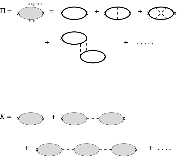
FIG. 1.: The diagrammatic representation of the linear response functions $\Pi$ and $K$. The response function $\Pi$ is the fully dressed fermion–hole bubble, irreducible with respect to a single gauge field line. The response function $K$ is the geometric series summing strings of bubbles connected by single gauge field propagator line. Solid lines are fermion propagators, while dashed lines are gauge field propagators. The physical meaning of both is discussed in the text.

FIG. 2.:

The self energy diagrams. (a.) The lowest order in $D$ diagram, leading to Eq. (14). The dashed line represents the RPA expression for the gauge field propagator (Eq. (12). (b.) The self consistent approximation, leading to Eq. (25).

FIG. 3.:

The proper interaction operator ${\tilde{\Gamma}}$ and the approximations we employ for it. (a.) The interaction operator $\Gamma$ is defined via the fermions’ two particle Green function $G^{(2)}$. In this figure, solid lines represent exact single particle Green’s functions. (b.) The simplest approximation for $\Gamma$, used in calculating Eq. (21). The dashed lines represent the RPA expression for the gauge field propagator (Eq. (12)), and the crosses represent bare vertices. The left diagram is proper, and is included in $\tilde{\Gamma}$. The right diagram is improper, and is not included in $\tilde{\Gamma}$. (c.) The ladder diagrams sum for ${\tilde{\Gamma}}$, summed in Appendix B.

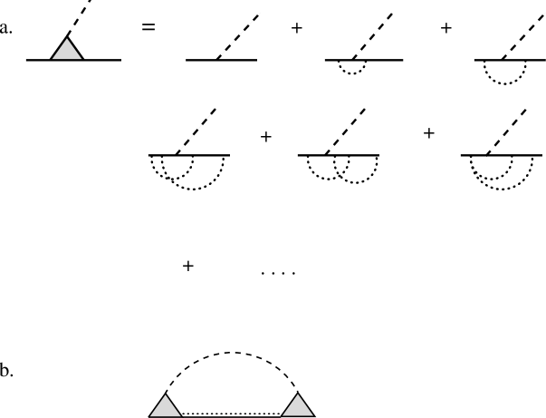
FIG. 4.:

(a.) Some low order contributions to the dressed vertex. The dashed line represents a low frequency long wavelength gauge field propagator. The dotted lines are short wavelength gauge field propagators. (b.) The renormalization of the self energy by short wavelength gauge field fluctuations. The dashed line carries the lowest momentum in the diagram. The double line (solid and dotted) denotes a fermion’s Green’s function, renormalized by the short wavelength gauge field fluctuations. As explained in text, the dominant contribution from the gauge field propagator is not expected to be renormalized.

FIG. 5.: The variation of the chemical potential when the density is varied, and $\Delta B$ is held fixed. The location of the origin and the units are arbitrary. Discontinuous jumps take place when a vacant Landau level starts being populated. Their magnitudes are the energy gaps for the corresponding fractional quantum Hall states. They reflect the value of $m^{*}$. Smooth variation takes place in between discontinuous jumps. The average slope of the curve is independent of the singular part of $m^{*}$.

REFERENCES

- [1] Future address (starting from October 1995): Department of Condensed Matter Physics, Weizmann Institute of Sciences, Rehovot 76100, Israel.
- [2] B.I. Halperin, P.A. Lee and N. Read, Phys. Rev. B 47, 7312 (1993).
- [3] A. Lopez and E. Fradkin Phys. Rev. B 44, 5246 (1991).
- [4] V. Kalmeyer and S.C. Zhang, Phys. Rev. B 46, 9889 (1992).
- [5] H.J. Kwon, A. Houghton and J.B. Marston, Phys. Rev. Lett. 73, 284 (1994).
- [6] Y.B. Kim, X.G. Wen, P.A. Lee and A. Furusaki, Phys. Rev. B 50 … (1994).
- [7] B.L. Altshuler, L. Ioffe and A.J. Millis, preprint.
- [8] J. Jain, Phys. Rev. Lett. 63, 199 (1989).
- [9] C. Nayak and F. Wilczek, Nuc. Phys. B417, 359 (1994).
- [10] C. Nayak and F. Wilczek, preprint.
- [11] J. Gan and E. Wong, Phys. Rev. Lett. 71, 4226 (1993).
- [12] J. Polchinski, Nucl. Phys. B422, 617 (1994); T. Holstein, R.E. Norton, and P. Pincus, Phys. Rev. B 8, 2649 (1973); M. Yu. Reizer, Phys. Rev. B 39, 1602 (1989); ibid. 40, 11571 (1989); B. Blok and H. Monien, Phys. Rev. B 47, 3454 (1993); D.V. Kveshchenko, R. Hlublina and T.M. Rice Phys. Rev. B 48, 10766 (1993); D.V. Kveshchenko and P.C.E. Stamp Phys. Rev. Lett. 71, 2118 (1993), Phys. Rev. B 49, 5227 (1994); P. Bares and X.G. Wen, Phys. Rev. B 48, 8636 (1993); Y.B. Kim and X.G. Wen, Phys. Rev. B 50, 8078 (1994); N. Nagaosa and P.A. Lee, Phys. Rev. Lett. 64, 2550 (1990); P.A. Lee and N. Nagaosa Phys. Rev. B 46, 5621 (1992); L.B. Ioffe and P.B. Wiegmann, Phys. Rev. Lett. 65, 653 (1990); L.B. Ioffe and G. Kotliar, Phys. Rev. B 42, 10348 (1990)C.M. Varma et.al., Phys. Rev. Lett. 63, 1996 (1989); P.W. Anderson, Phys. Rev. Lett. 65 2306 (1990); ibid. 66, 3226 (1991); ibid. 67, 2092 (1991); C.M. Varma, preprint; L. B. Ioffe, D. Lidsky and B.L. Altshuler, Phys. Rev. Lett. 73, 472 (1993); L.B. Ioffe and A.I. Larkin, Phys. Rev. B 39, 8988 (1989); P.A. Lee, Phys. Rev. Lett. 63, 680 (1989); S. Chakravarty, R.E. Norton and O.F. Syljuasen Phys. Rev. Lett. 74, 1423 (1995).
- [13] An equation in Ref. ([9]), suggesting a scaling of the form has been corrected to the relation in Ref. ([10]).
- [14] Unfortunately, there was a numerical error in the corresponding expression published in Ref. [2]. For the coefficient in Eq. (3) differs by a factor of from the value quoted in Ref. [2].
- [15] G.D. Mahan, Many Particle Physics, Plenum Press, New York (1981), Sec. 3.3.
- [16] E.M. Lifshitz and L.P. Pitaevskii, Statistical Physics, part 2, Pergamon Press. See in particular sections 18-19 and 64-65.
- [17] A.A. Abrikosov, L.P. Gorkov and I.E. Dzyaloshinski, Methods of quantum field theory in statistical physics, Dover publication, New York (1975)
- [18] P. Nozieres, Theory of interacting Fermi systems, W.A. Benjamin, New York, 1964. In particular, see chapters 1,5,6.
- [19] N. Read, Semicon. Sci. Tech. 9, 1859 (1994).
- [20] F.D.M. Haldane, Phys. Rev. Lett. 51, 605 (1983). See also S. Simon and B.I. Halperin, Phys. Rev. B 50, 1807 (1994).
- [21] C. Cohen–Tanoudji, B. Diu, F. Laloe, Quantum Mechanics, Wiley, New York (1977).
- [22] Y.B. Kim, X.G. Wen, P.A. Lee and P.C.E. Stamp, preprint.
- [23] S. Simon and B.I. Halperin, Phys. Rev. B 48, 17368 (1993).