Mobility in a one-dimensional disorder potential

Abstract

In this article the one-dimensional, overdamped motion of a classical particle is considered, which is coupled to a thermal bath and is drifting in a quenched disorder potential. The mobility of the particle is examined as a function of temperature and driving force acting on the particle. A framework is presented, which reveals the dependence of mobility on spatial correlations of the disorder potential. Mobility is then calculated explicitly for new models of disorder, in particular with spatial correlations. It exhibits interesting dynamical phenomena. Most markedly, the temperature dependence of mobility may deviate qualitatively from Arrhenius formula and a localization transition from zero to finite mobility may occur at finite temperature. Examples show a suppression of this transition by disorder correlations.

I Introduction

In recent years there has been wide interest in transport properties of disordered media: e.g. diffusion on a polymer in an external field, random resistor networks, domain wall dynamics of magnets in a random field, and pinning of vortices in type-II superconductors. Some reviews have already been devoted to this subject [1, 2, 3, 4].

This article focuses on the mobility of a particle moving at finite temperature in a one-dimensional disorder potential. Its purpose is twofold: (i) The functional dependence of mobility on temperature and on an additional external driving force is for the first time worked out explicitly in terms of stochastic properties of the disorder potential in the continuous space. Previous publications have mainly focused on the situation, where the particle moves on a lattice. The dynamics was specified in terms of hopping rates between neighbored places. Our point of view will be more adequate and also physically more transparent in situations, where the disorder potential is well characterized and hopping rates, if to be used, had to be calculated from this potential first. In other works, where space was treated as continuous, only special disorder types have been considered [5, 6]. (ii) This functional dependence is explicitly calculated and discussed for new models, in particular for spatially correlated distributions of the disorder force. Thereby we obtain generalizations of the Sinai model [7] with spatially uncorrelated forces, which has attracted particular attention in the past (see e.g. [5] and references therein).

Our approach, which leads to closed analytic expressions, is limited to the evaluation of the mean velocity. Thus interesting transport phenomena, like an anomalous scaling behavior of the (mean squared) displacement as a function of time, which characterize dynamical phases [4] and were found for the Sinai model [5, 6, 7, 8, 9], are beyond the scope of the present treatment.

In the following, we first derive and discuss the general expression for mobility (Sec. II). Its asymptotic behavior for large or small temperatures or driving forces is then analyzed (Sec. III). In Sec. IV mobility is calculated over the complete parameter range for some models. Finally, the phenomena of thermal activation encountered thereby are summarized (Sec. V).

II Basic description

Our problem is defined by the one-dimensional Langevin-equation for a single particle with coordinate $x$ in the presence of a disorder potential $U(x)$ and an external force $F$,

$$\dot{x}(t)=F-U^{\prime}(x(t))+\eta(t).$$ (1)

The thermal random force $\eta(t)$ is assumed to be Gaussian distributed with moments

$$\langle\eta(t)\rangle = 0,$$ (2a)

$$\langle\eta(t)\eta(t^{\prime})\rangle = 2T\delta(t-t^{\prime}).$$ (2b)

Angular brackets represent thermal average in a heat bath of temperature $T$.

We are interested in the velocity-force-characteristics (VFC) for a given disorder potential, where the average velocity is defined by

$$v_{T}(F):=\lim_{t\rightarrow\infty}\frac{1}{t}\ \overline{\langle x(t)-x(0)\rangle}.$$ (3)

A bar denotes the translation-average for the given realization of disorder, i.e. one replaces $U(x)$ by $U(x-x_{0})$ and averages over all $x_{0}$. In the last formula, this means an average over all initial positions $x(0)$. If desired, an additional average over an ensemble of disorder realizations should be taken as last operation.

For convenience, we suppose for the moment periodicity of the potential, $U(x+L)=U(x)$, and formulate the result in a way, which does not depend on the periodicity $L$. We argue then, that the result is correct for any unbiased disorder potential.

The dynamics of the model can be reformulated in terms of the Fokker-Planck equation for the probability density $P(t,x)$ and current density $J(t,x)$:

$$\partial_{t}P(t,x) = -\ \partial_{x}J(t,x),$$ (4a)

$$J(t,x) = \left[F-U^{\prime}(x)\right]P(t,x)-T\ \partial_{x}P(t,x).$$ (4b)

From the stationary solution, which has a homogeneous current distribution, one derives the mean velocity $v=JL/\int_{0}^{L}dxP(x)$ in a standard way (see e.g. [10])

$$v_{T}(F) = TL\left(1-e^{-LF/T}\right)/$$ (7)

$$/\Bigg{\{}\int_{0}^{L}dx\ e^{-\phi(x)/T}\int_{x}^{L}dx^{\prime}\ e^{\phi(x^{\prime})/T}+$$

$$+e^{-LF/T}\int_{0}^{L}dx\ e^{-\phi(x)/T}\int_{0}^{x}dx^{\prime}\ e^{\phi(x^{\prime})/T}\Bigg{\}}$$

with the effective potential $\phi(x):=U(x)-Fx$. This expression simplifies by replacing the periodicity $L$ by $NL$ and taking the limit $N\rightarrow\infty$. The result can be represented in two ways. A first one, frequently used in the literature, will be indicated in the following paragraph. The second one, which seemingly has been disregarded up to now and which can be evaluated more easily, is the basis of the remainder of this article.

The first version has the compact form

$$v_{T}(F)=\left[\ {\overline{\tau(x)}}\ \right]^{-1},$$ (8a)

where

$$\tau(x):=T^{-1}\int_{x}^{\pm\infty}dx^{\prime}\ e^{[\phi(x^{\prime})-\phi(x)]/T}$$ (8b)

with the integral running towards $\pm\infty$ for $F\mbox{\hbox{ \lower-2.58334pt\hbox{$>$}\kern-8.00003pt\lower 2.15277pt\hbox{$<$}\kern 3.50006pt}}0$. This representation of the VFC evaluates the so-called sojourn-time density $\tau(x)$: $dt=\tau(x)dx$ is proportional to the conditional probability of finding the particle in the interval $(x,x+dx)$ at times $t>0$, provided it started from position $x$ at $t=0$. Therein all later passages of the particle parallel and opposite to the direction of the driving force are included. Several works have been devoted to the study of sojourn-time distributions, mainly in spatially discrete hopping models (see e.g. [5] and references therein).

In contrast to Eq. (LABEL:VFC.1), which emphasizes the “dynamical” aspect of the problem by the statistical analysis of the sojourn-time, we prefer a second “static” point of view, formulated in terms of correlations of the disorder potential. This formulation enables us also to interpret our results directly in terms of activation processes in the energy landscape of the disorder potential. It is related to Eqs. (LABEL:VFC.1) by a mere change of the order of two integrations: the mobility

$$\mu_{T}(F):=v_{T}(F)/F$$ (9)

can be calculated directly as

$$\mu_{T}(F)=\left\{\int_{0}^{\infty}d\xi\ e^{-\xi}\ g_{T}(\xi T/F)\right\}^{-1}$$ (10a)

with the generating function

$$g_{T}(y):=\overline{\exp\left\{[U(x+y)-U(x)]/T\right\}}.$$ (10b)

Viewed as a function of temperature, $g_{T}(y)$ is the generating function of the potential energy difference correlations at distance $y$. Eq. (10a) shows, that mobility is essentially the Laplace transform of the generating function. In an experimental situation, where the force- and temperature dependence of mobility are known, the generating function may thus be determined by an inverse Laplace transformation.

The above derivation was based on the fact, that the current density is spatially constant in the stationary state, which is a particularity of one-dimensional problems. Unfortunately this approach does not allow an evaluation of the diffusion constant, which requires joint probability distributions at different times, and relaxation phenomena, which are not stationary. Both topics have been treated for the Sinai model[5, 6, 7, 8, 9].

Formulae (LABEL:VFC.1) and (LABEL:VFC.2) have been derived for periodic potentials. Since periodicity shows up only implicitly as a property of $\tau(x)$ and $g_{T}(y)$ but no longer explicitly as parameter, we postulate their validity also for non-periodic disorder potentials. Depending on the nature of disorder it may happen, that the stationary current is zero for some range of forces. In this case the integral in Eq. (10a) will diverge, leading to vanishing mobility.

In contrast to the original equation of motion, the expressions for the mobility are not invariant under the transformation $U(x)\rightarrow U(x)+const\times x$ and $F\rightarrow F+const$. They require an unbiased disorder potential, i.e.

$$\overline{U^{\prime}(x)}=0.$$ (11)

This condition, which is obvious for periodic potentials, has to be imposed on the non-periodic case as well. However, situations with a biased disorder potential can be treated, too. Then in our expressions $U$ has to be taken as the original potential after subtraction of its bias and $F$ as the original external force plus the mean force of the original potential.

For the spatially discrete version of the model with uncorrelated hopping rates, it was shown[11] that the results, obtained from a periodic potential and taking the limit of infinite periodicity in the end[8, 12], are unchanged, if one allows for non-periodicity from the very beginning. In addition, for zero temperature but arbitrary disorder, one can integrate the equation of motion Eq. (1) after separation of variables and finds directly the zero temperature limit of Eq. (10a) without use of periodicity, leading to Eq. (13) below.

Now we address the question, whether an additional average over different realizations of the disorder potential may affect the VFC. In principle, this average should be taken as last average in Eqs. (8a) or (10a). Again, for the spatially discrete version of the model with uncorrelated hopping rates, it was shown[11], that velocity is a self-averaging quantity. This means, that its value, when calculated for a given realization of the disorder potential, coincides with probability one with the value after an additional averaging over all realizations of the disorder potential. It seems natural to assume this property for any disorder potential with short-ranged correlations, since the particle samples during its drift the potential on infinite length scales, where a given realization is expected to be representative for the whole ensemble of realizations. Therefore we may consider the spatial averages as averages in the ensemble of disorder realizations. If, for a contrary example, the disorder extends only over a finite region, the ensemble-average does modify the result and is to be performed in addition. This situation has been studied for the Sinai model without bias[13].

Our main formula (LABEL:VFC.2) can be illustrated physically in the following way: Consider jumps over a finite distance $y$. The larger the fluctuations of $U(x+y)-U(x)$ when $x$ varies, the larger will be $g_{T}(y)\geq 1$. The inequality holds for all unbiased potentials. Therefore we might call $\Delta_{T}(y):=T^{-1}\ln g_{T}(y)\geq 0$ “energetic roughness” on distances $y$. A large roughness signifies a pronounced relief-structure of the potential to be overcome by thermal activation and reduces mobility. An “enthalpic roughness” $\hat{\Delta}_{T}(F)$ can be introduced by $\exp[\hat{\Delta}_{T}(F)/T]:=(T/F)\int_{0}^{\pm\infty}dy\exp[-yF/T+\Delta_{T}(y)/T]$, reminding of the relation between free energy and enthalpy in equilibrium thermodynamics, since $F$ and $y$ are thermodynamically conjugated variables. This enthalpic roughness turns out to act as an effective activation energy, since it determines mobility by $\mu_{T}(F)=\exp[-\hat{\Delta}_{T}(F)/T]$.

Eq. (LABEL:VFC.2) shows also, that in the evaluation of the disorder potential an energy scale is set by temperature, whereas the spatial structure of the potential is relevant only up to the length scale $T/F$.

III Limiting cases

Before we attempt to evaluate the VFC for particular models, defined by a probability distribution of the disorder potential, we analyze different limits of the general expression for mobility.

A Low temperatures

At strictly zero temperature, we obtain from an integration of the equation of motion (1) over a finite time interval $(t_{i},t_{f})$:

$$\frac{x_{f}-x_{i}}{t_{f}-t_{i}}=F\ \frac{x_{f}-x_{i}}{\int_{x_{i}}^{x_{f}}\frac{dx}{1-U^{\prime}(x)/F}},$$ (12)

with $x_{i,f}=x(t_{i,f})$. If the disorder force is everywhere weaker than the external force, $U^{\prime}(x)/F<1$, the particle cannot be trapped in the disorder potential. In the limit $t_{f}-t_{i}\rightarrow\infty$, Eq. (12) then confirms the zero-temperature limit of Eq. (LABEL:VFC.2):

$$\mu_{T}(F)=\left\{\overline{[1-U^{\prime}(x)/F]^{-1}}\right\}^{-1}.$$ (13)

In the opposite case, with $U^{\prime}(x)/F>1$ somewhere, the particle will be localized, i.e. have vanishing mobility. The threshold-forces $F_{c}^{\pm}$ for the onset of drift towards $x=\pm\infty$ are clearly given by the maximum/minimum slope of $U$. In the localized region, Eq. (12) is invalid in the strict sense, since the particle does no longer sample the whole potential. However, if it is used naively, localization formally shows up by a divergence of the integral in the denominator.

At small, but finite temperatures, one might expect to find an Arrhenius-like thermally activated behavior. This is certainly true for periodic potentials, where one easily derives (for $F\mbox{\hbox{ \lower-2.58334pt\hbox{$<$}\kern-8.00003pt\lower 2.15277pt\hbox{$>$}\kern 3.50006pt}}F_{c}^{\pm}$)

$$v=L\frac{\sqrt{-\lambda_{\max}\lambda_{\min}}}{2\pi}\ e^{-[\phi(x_{\max})-\phi(x_{\min})]/T}$$ (14)

with $\lambda_{\max,\min}:=\phi^{\prime\prime}(x_{\max,\min})$, where $x_{\min/\max}$ denotes the position of a minimum/maximum of $\phi$ such, that $(x_{\max}-x_{\min})/F>0$ and the energy difference $\phi(x_{\max})-\phi(x_{\min})$ is maximal. This expression is valid only for temperatures much smaller than this activation energy and $L|F|/T\gg 1$, such that activation over the maximum occurs only in the direction of $F$. In this case, the mean velocity is just proportional to Kramers transition rate (see e.g. [14]) for thermal activation out of minimum $x_{\min}$ over $x_{\max}$. The resulting velocity is finite for all finite external forces.

In the case of non-periodic disorder potentials, where arbitrarily large energy barriers (or curvatures at extrema) occur with finite probability density and thus no highest energy barrier exists, deviations from Arrhenius-like temperature dependence may occur.

B High temperatures

For high temperatures one may expand the generating function into

$$g_{T}(y)=\sum_{n=0}^{\infty}\frac{1}{n!}T^{-n}\ \overline{[U(x+y)-U(x)]^{n}}.$$ (15)

An additional temperature dependence of mobility comes in through the fact, that the generating function is evaluated at distances $y=\xi T/F$, which increase with temperature. If qualitatively $\overline{[U(x+y)-U(x)]^{n}}\sim|y|^{n\zeta}$ for $|y|\rightarrow\infty$ with some roughness exponent $\zeta<1$, we will have anyway

$$\mu_{T}(F)=1-{\cal O}\left(T^{2(\zeta-1)}\right).$$ (16)

On the other hand, if the potential is so rough that $\zeta>1$, this series diverges and the particle can be expected to be localized at all temperatures.

C Small driving forces

In the limit of small $F$, the function $g_{T}(y)$ is evaluated in (10a) mainly for large arguments and the integral therein acts as additional spatial average. Then one has

$$\mu_{T}(F)\approx\left[\overline{e^{U(x)/T}}\ \ \overline{e^{-U(x)/T}}\right]^{-1},$$ (17)

provided that the averages therein exist. Therefore, one has finite mobility $0<\mu\leq 1$ for small driving forces, i.e. Ohmic behavior. The range of this Ohmic regime is given by the condition, that $T/F$ has to be small compared to typical length scales (periodicity or correlation length) of the disorder. Remarkably, mobility is independent of the direction of the driving force, even for asymmetric potentials. If, on the other hand, one of the averages is infinite, mobility vanishes for small forces. In general, any non-Ohmic behavior requires the divergence of one of the averages in Eq. (17).

It is interesting to note, that a disorder potential may give rise to a temperature dependence of the Ohmic mobility, which is qualitatively different from Arrhenius-like behavior. In order to illustrate this, let us assume a potential energy density

$$P(U_{1}):=\overline{\delta(U_{1}-U(x))}$$ (18)

with an asymptotics

$$P(U)\approx c\exp\left[-|U/E|^{\sigma}\right]$$ (19)

for $U\rightarrow\pm\infty$ with some energy scale $E$ and exponent $\sigma>1$. For small temperatures we may evaluate the integrals in Eq. (17) with a saddle-point approximation and obtain

$$\mu_{T}(F) \approx \frac{\sigma(\sigma-1)}{2\pi c^{2}E^{2}}\left(\frac{E}{\sigma T}\right)^{(\sigma-2)/(\sigma-1)}\times$$ (21)

$$\times\exp\left[-2(\sigma-1)\left(\frac{E}{\sigma T}\right)^{\sigma/(\sigma-1)}\right].$$

Only in the limit $\sigma\rightarrow\infty$, i.e. a narrow distribution $P(U)$, one obtains an Arrhenius-like temperature dependence of the velocity. Potentials of a finite width, like periodic or quasiperiodic ones, belong to this class. For general $\sigma>1$, mobility will vanish with temperature faster than Arrhenius-like, since the exponent $\sigma/(\sigma-1)$ in the exponential function will be greater than one. However, for $\sigma>1$ and $T>0$ mobility will always be finite.

In the marginal case $\sigma=1$ we find a transition from zero mobility at $T\leq E$ to finite mobility at $T>E$. In the case $\sigma<1$ the particle will always have zero mobility.

These results show the naively expected tendency: the broader the distribution $P(U)$, the larger are the involved activation energies and the smaller is the mobility. Perhaps less expected is the fact, that spatial correlations of the potential for small $y$ will affect the VFC only for larger driving forces.

D Large driving forces

In the limit of large $F$, the function $g_{T}(y)$ is evaluated in Eq. (10a) only for small arguments. We now expand

$$g_{T}(\xi T/F)=1+(F_{c1}^{\pm}/F)\ \xi+\frac{1}{2}(F_{c2}^{\pm}/F^{2})\ \xi^{2}+\dots$$ (22)

for $\xi\mbox{\hbox{ \lower-2.58334pt\hbox{$>$}\kern-8.00003pt\lower 2.15277pt\hbox{$<$}\kern 3.50006pt}}0$, where we introduced in general temperature-dependent characteristic forces of order $n$ by

$$F_{cn}^{\pm}:=\left.\left(T\frac{d}{dy}\right)^{n}g_{T}(y)\right|_{y=0^{\pm}}.$$ (23)

From the representation (10a) for the mean velocity, we obtain

$$\mu_{T}(F)\approx\frac{1}{1+F_{c1}^{\pm}/F+F_{c2}^{\pm}/F^{2}+\dots}$$ (24)

If the nature of the disorder potential is “smooth”, i.e. allows to change the order of differentiation an averaging, one derives from the definition (10b) of $g$, that

$$F_{c1}^{\pm} = \overline{U^{\prime}(x)}=0,$$ (25a)

$$F_{c2}^{\pm} = \overline{TU^{\prime\prime}(x)+U^{\prime 2}(x)}>0.$$ (25b)

If in addition $\overline{U^{\prime\prime}(x)}=0$, as for periodic potentials, the leading correction of the asymptotics is temperature-independent.

Otherwise, if the potential is not smooth, the identities (LABEL:Fcn.smooth) need not hold, as we will see in the Gaussian model below, where $F_{c1}^{\pm}$ may be different from zero. Then disorder affects a finite shift of velocity with respect to the disorder-free case even for large velocities,

$$v_{T}(F\rightarrow\pm\infty)=F-F_{c1}^{\pm}+{\cal O}(F^{-1})$$ (26)

for $F^{2}\gg F_{c2}^{\pm}$.

In the case of a discontinuous potential, one may find $g_{T}(0^{\pm})\neq 1$ inhibiting the expansion (22), see e.g. the random-potential case of the Gaussian model below.

IV Examples

We now explicitly calculate the VFC for certain disorder potentials to demonstrate the richness of phenomena which can be found in this class of diffusion problems.

A Sinusoidal model

For the sake of completeness, let us discuss in the present context the periodic model $U(x)=E\sin(2\pi x/L)$, which has been studied already some time ago by Ambegaokar and Halperin[15] in order to determine the thermal noise contribution to the dc Josephson effect. Afterwards, we will discuss a non-periodic generalization of this model.

The generating function can easily be calculated as

$$g_{T}(y)=I_{0}\left[2(E/T)\sin(\pi y/L)\right],$$ (27)

where $I_{0}$ is a modified Bessel function. Due to the smoothness and symmetry of the potential, $g_{T}(y)$ is even and analytic. A straightforward evaluation of Eq. (10a) leads to

$$\mu_{T}(F) = \frac{\sinh\pi f/\vartheta}{\pi f/\vartheta}\ \Bigg{\{}\int_{0}^{1}d\xi\times$$ (29)

$$\times\cosh[\xi\pi f/\vartheta]\ I_{0}[(2/\vartheta)\cos(\xi\pi/2)]\Bigg{\}}^{-1}$$

with reduced temperature $\vartheta:=T/E$ and reduced force $f:=F/F_{0}$ where $F_{0}:=2\pi E/L$. This expression can be treated further analytically only in limiting cases. The result of its numerical integration is shown in Fig. 1.

At $T=0$ one finds from Eq. (13)

$$\mu_{0}(F)=\left\{\begin{array}[]{ll}0&{\rm for}\quad|f|\leq 1\\ \sqrt{1-f^{-2}}&{\rm for}\quad|f|>1\end{array}\right.$$ (30)

with a rapid onset of motion near the the critical force $F_{c}:=\max_{x}[|U^{\prime}(x)|]=F_{0}$.

At low temperatures and within the force-region $|f|<1$, where the particle is localized at zero temperature, we find from an saddle-point evaluation of Eq. (29)

$$v_{T}(F) = 2F_{0}\ \sinh(\pi f/\vartheta)\ \sqrt{1-f^{2}}\ \ e^{-E_{A}(F)/T}$$ (31a)

$$E_{A}(F) := 2E\sqrt{1-f^{2}}+2Ef\arcsin f,$$ (31b)

provided $\vartheta\ll\sqrt{1-f^{2}}$ and $\vartheta\ll f\arcsin f$. The temperature range of its validity shrinks when the external force vanishes or approaches the critical force. This asymptotic evaluation yields the mean velocity just as the difference of Kramers rates for an activation parallel and antiparallel to the driving force across energy barriers $E_{A}(F)\mp\pi fE$. Since the energy barriers assume only certain values, temperature dependence is Arrhenius-like.

At high temperatures, we can expand the denominator of Eq. (29) in $E/T$. This produces only even terms and we find to second order

$$\mu_{T}(F)\approx\left\{1+\frac{2(E/T)^{2}}{4+(2fE/T)^{2}}\right\}^{-1}.$$ (32)

At small forces follows from Eq. (29)

$$\mu_{T}(F)\approx[I_{0}(E/T)]^{-2}$$ (33)

in agreement with a direct calculation from Eq. (17) with

$$\overline{e^{\pm U(x)/T}}=I_{0}(E/T).$$ (34)

The characteristic forces of lowest order are $F_{c1}^{\pm}=0$ and $F_{c2}^{\pm}=F_{0}^{2}/2$, since $U$ is smooth. In Fig. 1 one observes for finite temperatures, that the VFC approaches in the limit $F\rightarrow\infty$ first the curve $T=0$ before it assumes the limit $\mu=1$. This reflects the fact, that the leading correction to $\mu=1$ is temperature-independent.

Now we address the question, how these results will change when the periodicity of the potential is abandoned. Let us construct such a potential by stretching the maxima $U=E$ from points to plateaus such, that the density of minima $U=-E$ is reduced to $\rho<1/L$. The generating function $g_{T}(y)$ behaves for small $y$ as

$$g_{T}(y)\approx(1-\rho L)+\rho LI_{0}\left[2(E/T)\sin(\pi y/L)\right],$$ (35)

since this distance falls with probability $(1-\rho L)$ onto a plateau and with probability $\rho L$ into a trap region with $U<E$, where Eq. (27) holds. This expression is correct in ${\cal O}(y^{2})$, thus the leading correction for large driving forces is given by

$$F_{c2}^{\pm}=2\rho L(\pi E/L)^{2}$$ (36)

and vanishes with density $\rho$. However, the critical force $F_{c}=2\pi E/L$ at $T=0$, being the maximum slope of $U$, does not depend on $\rho$. On the other hand, if there is no long-range translational order between the traps, we deduce using Eq. (34)

$$\overline{e^{\pm U(x)/T}}\approx(1-\rho L)e^{\pm E/T}+\rho LI_{0}(E/T).$$ (37)

and the asymptotics

$$\mu_{T}(F\rightarrow 0) \approx \big{[}2(1-\rho L)\rho L\sinh(E/T)I_{0}(E/T)+$$ (39)

$$+(1-\rho L)^{2}+\rho^{2}L^{2}I_{0}^{2}(E/T)\big{]}^{-1}.$$

This expression displays a low-temperature behavior

$$\mu_{T}(F\rightarrow 0) \approx \left[(1-\rho L)\rho L\sqrt{2\pi E/T}+\rho^{2}L^{2}\right]^{-1}\times$$ (41)

$$\times 2\pi(E/T)e^{-2E/T}.$$

Its exponential factor is Arrhenius-like with activation energy $2E$. The prefactor can not be calculated from Kramers expression (14), since the curvature of the maximum is infinite. Remarkably, mobility at zero force and its leading correction at large forces depend only on the mean density of traps and not on more information about their distribution. This is true for any shape of the traps, at small forces since $\overline{\exp[\pm U(x)/T]}$ depends only on the shape and density of traps, at large forces since the leading term of $g_{T}(y)-1$ for small $y$ is simply proportional to the density.

B Gaussian model

In general, the probability distribution ${\cal P}$ of the functions $U$ may be generated by an “hamiltonian” ${\cal H}$,

$${\cal P}[U]\propto\exp\{-{\cal H}[U]\}.$$ (42)

The hamiltonian can have direct physical significance. Imagine that the particle diffuses on a substrate. In an external field, the shape of this substrate will determine the energy $U$ of the particle. Assume that the shape of the substrate was frozen after a quench from an initial temperature, where the substrate performed shape-fluctuations according to a reduced hamiltonian ${\cal H}$ (substrate energy divided by temperature). Then this hamiltonian determines the distribution of potentials $U$ according to Eq. (42).

In this section we consider the Gaussian case, where the hamiltonian is bilinear in the potential. We assume the “energy” of a realization of the potential to be determined by a inversion-symmetric stiffness $\epsilon$ in Fourier-space according to

$${\cal H}[U]=\frac{1}{2}\int\frac{dk}{2\pi}\ U(k)\epsilon(k)U(-k),$$ (43)

for which one obtains immediately

$$g_{T}(y)=\exp\left\{\frac{1}{T^{2}}\int\frac{dk}{2\pi}\ \frac{1-\cos(ky)}{\epsilon(k)}\right\}.$$ (44)

The stiffness should satisfy $\lim_{k\rightarrow 0}k^{3}/\epsilon(k)=0=\lim_{k\rightarrow\infty}k/\epsilon(k)$, otherwise the particle is always localized. We restrict us to $\epsilon(k)=m_{0}+m_{1}|k|+m_{2}k^{2}$, thereby generalizing Sinai’s random-force model with a term $m_{2}k^{2}$ only. For simplification we select the cases with $m_{1}=0$ or $m_{0}=0$.

We start with $m_{1}=0$, where the absolute fluctuations of $U(x)$ are confined. One has

$$g_{T}(y)=\exp\left\{\left(1-e^{-|y|/y_{0}}\right)y_{0}F_{T}/T\right\}$$ (45)

with the length- and force-scales

$$y_{0} := \sqrt{m_{2}/m_{0}},$$ (46a)

$$F_{T} := 1/2m_{2}T.$$ (46b)

Since the potential now typically is rough on short length scales, $g_{T}(y)$ has a non-analytic distance dependence at $y=0$. In addition, the first characteristic force

$$F_{c1}^{\pm}=\pm F_{T}$$ (47)

is finite and depends on temperature, as well as the characteristic forces of higher order.

Laplace integration over $g$ yields (see Fig. 2a)

$$\mu_{T}(F)=\frac{1}{y_{0}|F|/T}\frac{(y_{0}F_{T}/T)^{y_{0}|F|/T}\ e^{-y_{0}F_{T}/T}}{\gamma(y_{0}|F|/T,y_{0}F_{T}/T)},$$ (48)

where $\gamma$ denotes the incomplete gamma function. This model exhibits the asymptotic behavior

$$\mu_{T}(F\rightarrow\pm\infty) = 1-F_{T}/|F|,$$ (49a)

$$\mu_{T}(F\rightarrow 0) = \exp\{-y_{0}F_{T}/T\}.$$ (49b)

It provides an explicit example of a non-Arrhenius-like temperature dependence of the mobility, since $y_{0}F_{T}/T=1/(2\sqrt{m_{0}m_{2}}\ T^{2})$. The fact, that temperature occurs squared, is due to the Gaussian nature of disorder in agreement with the discussion leading to Eq. (21). Note, that the limit $F\rightarrow 0$ always contains the constant $m_{2}$, which enters the distribution

$$P(U) \propto \exp\left\{-\frac{U^{2}}{2}\left[\int\frac{dk}{2\pi\epsilon(k)}\right]^{-1}\right\}=$$ (50a)

$$= \exp\{-\sqrt{m_{0}m_{2}}\ U^{2}\}.$$ (50b)

It would be therefore misleading to reason, that this limit should depend only on $m_{2}$, which governs $\epsilon(k)$ for small $k$. Rather, for this limit all length scales matter, as already visible in Eq. (44).

The special case $m_{1}=m_{2}=0$ describes an uncorrelated potential and Eq. (17) applies for all forces. As the amplitude of fluctuations diverges in the limit $m_{2}\rightarrow 0$, the generating function diverges since $\lim_{k\rightarrow\infty}k/\epsilon(k)\neq 0$ and the particle is localized at all temperatures and driving forces.

Consider now the case $m_{0}=0$, where

$$g_{T}(y) = \exp\{(2y_{1}F_{T}/\pi T)[C+\ln|y/y_{1}|-$$ (52)

$$-{\rm ci}\ |y/y_{1}|\cos|y/y_{1}|-{\rm si}\ |y/y_{1}|\sin|y/y_{1}|]\}$$

$$\approx \left(e^{C}|y/y_{1}|\right)^{(2y_{1}F_{T}/\pi T)}$$ (53)

with a length-scale $y_{1}:=m_{2}/m_{1}$, the force-scale $F_{T}:=1/2m_{2}T$ as before, Eulers constant $C=0.577\dots$, and the cosine and sine integrals ${\rm ci}$ and ${\rm si}$. Fig. 2b shows mobility obtained by numerical integration of Eq. (52). The approximation in Eq. (53) refers to $|y/y_{1}|\gg 1$. The power-law behavior of $g$ for large $y$ translates under Laplace transformation to a power-law behavior for small $F$:

$$\mu_{T}(F) \approx \frac{\left(e^{-C}y_{1}|F|/T\right)^{(2y_{1}F_{T}/\pi T)}}{\Gamma[(2y_{1}F_{T}/\pi T)+1]}$$ (54)

$$\rightarrow \frac{1}{\sqrt{4y_{1}F_{T}/T}}\left(\pi e^{1-C}|F|/2F_{T}\right)^{(2y_{1}F_{T}/\pi T)}$$ (55)

$\Gamma$ denotes the gamma function, the approximation is valid for $F\ll F_{T}$, the limit refers to $T\rightarrow 0$. Since the exponent $2y_{1}F_{T}/\pi T=1/\pi m_{1}T^{2}$ is positive, the mobility always vanishes with $F$. The exponent is independent of the parameter $m_{2}$. Mobility behaves at low temperatures like $T^{1/\pi m_{1}T^{2}}$. In this case, we observe an even stranger deviation from Arrhenius-activation. Since ${\cal P}[U]$ is invariant under $U(x)\rightarrow U(x)+const$, the potential is unbound and Eq. (21) is violated.

The case $m_{0}=m_{2}=0$ again leads to complete localization, since $\lim_{k\rightarrow\infty}k/\epsilon(k)\neq 0$.

The case $m_{0}=m_{1}=0$ is, as already indicated above, the Sinai random-force model[7]. To show the equivalence of our approach with the discrete approaches[8, 11], we reproduce the VFC of this case. Eq. (45) reduces to

$$g_{T}(y)=\exp\left\{|y|F_{T}/T\right\}$$ (56)

for all $y$ and results in (compare Fig. 2c)

$$\mu_{T}(F)=\left\{\begin{array}[]{ll}0&{\rm for}\quad|F|\leq F_{T}\\ 1-F_{T}/|F|&{\rm for}\quad|F|>F_{T}.\end{array}\right.$$ (57)

Therefore $F_{T}$ is the threshold force for the onset of motion. The temperature dependence of the model is completely contained in this threshold force. In particular, one finds at constant $F$ a localization transition at temperature $T_{c}=1/2m_{2}F$.

All cases with $m_{2}\neq 0$ discussed above have a common asymptotics for large driving forces, which is determined by $m_{2}$ alone. The reason therefore is, that this asymptotics is governed only by the short-scale fluctuations of the potential, determined by leading term of the stiffness for large $k$.

C Poissonian model

Finally, we consider a model for diffusion on a stepped crystalline surface, as illustrated in Fig. 3a. This model shows asymmetric transport properties and also exhibits a localization transition.

The profile of the surface is described by the height function $h(x)$, which increases in units of $a>0$ for increasing $x$. The structure is characterized by the probability distribution $S(l)$ for the step length $l$. We use a Poisson-distribution $S(l)=\exp(-l/l_{0})/l_{0}$ with mean value $l_{0}$. The particle is supposed to be in constant force-field with components $f_{x,h}$ in direction parallel and perpendicular to the $x$-direction, which might be components of a gravitational or electric field. They give rise to the total potential $\phi(x)=f_{h}h(x)-f_{x}x$. In order to use our previous formulae, we identify $U(x)=f_{h}h(x)-(a/l_{0})f_{h}x$ and $F=f_{x}-(a/l_{0})f_{h}$ by subtracting the mean bias.

From the Poissonian distributed number of steps in an interval of length $y$ one obtains easily

$$g_{T}(y)=\exp[yF_{c1}^{\pm}(T)/T]$$ (58)

for $\xi\mbox{\hbox{ \lower-2.58334pt\hbox{$>$}\kern-8.00003pt\lower 2.15277pt\hbox{$<$}\kern 3.50006pt}}0$ with asymmetric forces of first order

$$F_{c1}^{\pm}(T)=-(a/l_{0})f_{h}\mp(1-e^{\pm af_{h}/T})T/l_{0}\mbox{\hbox{ \lower-2.58334pt\hbox{$>$}\kern-8.00003pt\lower 2.15277pt\hbox{$<$}\kern 3.50006pt}}0,$$ (59)

which depend on temperature. From Eq. (58) we obtain (see Fig. 3b)

$$\mu_{T}(F)=\left\{\begin{array}[]{ll}0&{\rm for}\quad F_{c1}^{-}(T)<F<F_{c1}^{+}(T),\\ 1-F_{c1}^{\pm}(T)/F&{\rm for}\quad F\mbox{\hbox{ \lower-2.58334pt\hbox{$>$}\kern-8.00003pt\lower 2.15277pt\hbox{$<$}\kern 3.50006pt}}F_{c1}^{\pm}(T).\end{array}\right.$$ (60)

Since at $T=0$ the localization region covers $-(a/l_{0})f_{h}<F<\infty$ (corresponding to $0<f_{x}<\infty$) and shrinks to zero for $T\rightarrow\infty$, we find for forces in this region a localization transition at a temperature $T_{c}$, which is implicitly determined by $F=F_{c1}^{\pm}(T)$, as depicted in Fig. 3c.

Apart from the asymmetry, the Poissonian model is very similar to the random-force Gaussian model. Indeed, the force is distributed independently at different sites, this time, however, with an asymmetric and singular distribution.

V Conclusion

An analysis of particle mobility in one-dimensional disorder was presented. We developed a framework based on the generating function of spatial correlations of the disorder potential. For arbitrary temperature and driving force, these correlations are relevant up to a length $T/F$. At large driving forces, mobility depends only on local properties of disorder, whereas at small driving forces global aspects matter.

For some models, which generalize previously studied structures of disorder, mobility was evaluated over the complete range of temperature and force. Thermally activated motion led to a rich phenomenology.

The temperature-dependence of mobility can deviate drastically from Arrhenius formula. This is characteristic for systems with a broad distribution of activation energies. Such deviations have been obtained already by an ad hoc averaging of escape times over a spectrum of activation energies (see e.g. [16]). This procedure is unsatisfying from a principal point of view, since transport properties depend also on the spatial location and not only on the height of energy barriers, which is in higher dimensions even more important than in one dimension.

The models with spatially uncorrelated force distribution, the Poissonian model as well as the random-force Gaussian model, exhibit a localization transition. The similar phenomenology of these models is due to the validity of the Central Limit Theorem, which assures a Gaussian distribution of $U(x+y)-U(x)$.

It is therefore of particular interest to examine the stability of the localization phases with respect to the introduction of correlations in the force-distribution. For the Gaussian model, we achieved this by two different, continuous deformations of the random-force model. Switching on the couplings $m_{0}$ or $m_{1}$, we found the localized phase to be unstable, i.e. mobility was finite for all positive temperatures and driving forces.

This result complements previous studies: In a dynamics, where the particle may hop on a lattice only in one direction and which is thus incompatible with a Langevin equation of motion, dynamical phases were found to be stable with respect to short-ranged correlations in the hopping rates, but unstable with respect to long-ranged correlations[17]. Introducing force-correlations into the Sinai model, the scaling behavior of diffusion in the absence of a driving fore has been found to be modified, but remained anomalous[18, 19].

VI Acknowledgements

I am grateful to P. Nozières for a critical reading of the manuscript and to N. Pottier and D. Saint-James for interesting comments.

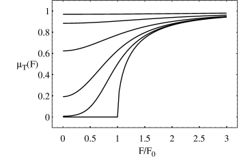
FIG. 1.: Mobility of the sinusoidal model according to Eq. (29) as a function of the driving force for $T/E=4$, 2, 1, 0.5, 0.25, 0 from top to bottom.

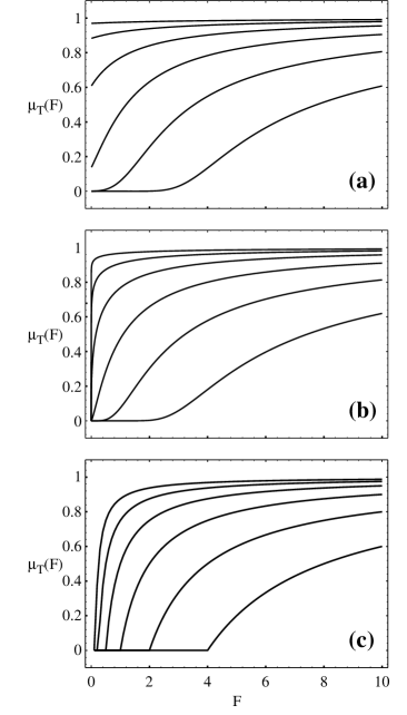
FIG. 2.: Mobility of the Gaussian model as a function of the driving force for different temperatures $T=4$, 2, 1, 0.5, 0.25, 0.125 from top to bottom in each diagram: (a) for $m_{0}=m_{2}=1$ according to Eq. (48), (b) for $m_{1}=m_{2}=1$ after numerical Laplace integration of Eq. (52), and (c) for the random force model as limiting case $m_{0}=m_{1}=0,m_{2}=1$.

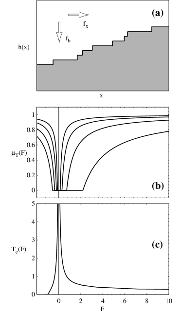
FIG. 3.: Poissonian model: (a) sketch of geometry, (b) mobility according to Eq. (60) as a function of the driving force at temperatures $T=4$, 2, 1, 0.5 from top to bottom and (c) localization temperature as a function of driving force for $af_{h}=l_{0}=1$.

REFERENCES

- [1] S. Alexander, J. Bernasconi, W.R. Schneider, and R. Orbach, Rev. Mod. Phys. 53, 175 (1981).
- [2] J.W. Haus and K.W. Kehr, Phys. Rep. 150, 263 (1987).
- [3] S. Havlin and D. Ben-Avraham, Adv. Phys. 36, 695 (1987).
- [4] J.-P. Bouchaud and A. Georges, Phys. Rep. 195, 127 (1990).
- [5] J.P. Bouchaud, A. Comtet, A. Georges, and P. Le Doussal, Ann. Phys. 201, 285 (1990).
- [6] C. Aslangul, M. Barthélémy, N. Pottier, and D. Saint-James, Physica A 171, 47 (1991).
- [7] Ya. G. Sinai, in: Lecture Notes in Physics Vol. 153, R. Schrader, R. Seiler, and D.A. Uhlenbrock eds. (Springer, Berlin 1981); Theor. Prob. Appl. 27, 256 (1982).
- [8] B. Derrida and Y. Pomeau, Phys. Rev. Lett. 48, 627 (1982); B. Derrida, J. Stat. Phys. 31, 433 (1983).
- [9] J.P. Bouchaud, A. Comtet, A. Georges, and P. Le Doussal, Europhys. Lett. 3, 653 (1987).
- [10] H. Risken: “The Fokker-Planck Equation”, Springer, Berlin (1984).
- [11] C. Aslangul, J.-P. Bouchaud, A. Georges, N. Pottier, and D. Saint-James, J. Stat. Phys. 55, 461 (1989).
- [12] C. Aslangul, N. Pottier, and D. Saint-James, J. Phys. France 50, 899 (1989).
- [13] G. Oshanin, A. Mogutov, and M. Moreau, J. Stat. Phys. 73, 379 (1993).
- [14] P. Hänggi, P. Talkner, and M. Borkovec, Rev. Mod. Phys. 62, 251 (1990).
- [15] V. Ambegaokar and B.I. Halperin, Phys. Rev. Lett. 22, 1364 (1969).
- [16] T.A. Vilgis, J. Phys. C 21, L299 (1988).
- [17] C. Aslangul, N. Pottier, P. Chvosta, and D. Saint-James, Europhys. Lett. 19, 347 (1992); Phys. Rev. E 47, 1610 (1993).
- [18] J.P. Bouchaud, A. Comtet, A. Georges, and P. Le Doussal, J. Physique 48, 1445 (1987).
- [19] S. Havlin, M. Schwarz, R.B. Selinger, A. Bunde, and H.E. Stanley, Phys. Rev. A 40, 1717 (1989).