Elastic theory of flux lattices in presence of weak disorder

Abstract

The effect of weak impurity disorder on flux lattices at equilibrium is studied quantitatively in the absence of free dislocations using both the Gaussian variational method and the renormalization group. Our results for the mean square relative displacements $\tilde{B}(x)=\overline{\langle u(x)-u(0)\rangle^{2}}$ clarify the nature of the crossovers with distance. We find three regimes: (i) a short distance regime (“Larkin regime”) where elasticity holds (ii) an intermediate regime (“Random Manifold”) where vortices are pinned independently (iii) a large distance, quasi-ordered regime where the periodicity of the lattice becomes important. In the last regime we find universal logarithmic growth of displacements for $2<d<4$: $\tilde{B}(x)\sim A_{d}\log|x|$ and persistence of algebraic quasi-long range translational order. The functional renormalization group to $O(\epsilon=4-d)$ and the variational method, when they can be compared, agree within $10\%$ on the value of $A_{d}$. In $d=3$ we compute the function describing the crossover between the three regimes. We discuss the observable signature of this crossover in decoration experiments and in neutron diffraction experiments on flux lattices. Qualitative arguments are given suggesting the existence for weak disorder in $d=3$ of a “ Bragg glass ” phase without free dislocations and with algebraically divergent Bragg peaks. In $d=1+1$ both the variational method and the Cardy-Ostlund renormalization group predict a glassy state below the same transition temperature $T=T_{c}$, but with different $\tilde{B}(x)$ behaviors. Applications to $d=2+0$ systems and experiments on magnetic bubbles are discussed.

I Introduction

The interest in the pinning of the Abrikosov vortex lattice by impurities was revived recently with the discovery of high-Tc superconductors. Impurity disorder conflicts with the long range translational order of the flux lattice and some glassy state is generally expected to appear. Understanding the precise nature of this new thermodynamic state and how it depends on the type of disorder existing in the system is very important for the determination of the transport properties of these materials, such as critical currents and I-V characteristics [3, 4, 5, 6, 7]. This problem, however, is only one aspect of the more fundamental and broader question of the effect of quenched impurities on any translationally ordered structure, such as a crystal. This question arises in a large number of physical systems under current active experimental study. Examples are charge density waves [8], Wigner crystals [9, 10, 11, 12] magnetic bubbles [13, 14], Josephson junctions [15, 16], the surface of crystals with quenched bulk or substrate disorder [17], domain walls in incommensurate solids [18]. All these systems have in common a perfectly ordered underlying structure modified by elastic distortions and possibly by topological defects such as dislocations, due to temperature or disorder. The effect of thermal fluctuations alone on three-dimensional and especially on two-dimensional structures is by now well understood, and it was shown that topological defects are not important in the low temperature solid phase [19]. Much less is known however on the additional effects of quenched disorder. In particular, the important question of precisely how quenched disorder destroys the translational long range order of the lattice is far from being elucidated. If disorder is strong, the underlying order is a priori destroyed at every scale and an analytical description of the problem starting from the Abrikosov lattice is difficult. One then has to use a more macroscopic approach based on phenomenological models such as the gauge glass models [4, 20, 21]. The success of these approaches then crucially depends on whether these effective models are indeed a good representation of the system at large scale, a largely uncontrolled assumption. If disorder is weak enough, however, one expects the perfect lattice to survive at short scales. Thus a natural first step for a theoretical description is to neglect dislocations and to treat the simpler problem of an elastic medium submitted to weak impurities. In that case one can consider a gaussian random potential created by many weak impurities with short-range correlations. In this paper we will focus on point-like disorder. The problem of correlated disorder, such as columnar or twin boundary pinning in superconductors [5, 6], which is also relevant for any type of quantum problems can be treated by similar methods, and is examined in details in Ref. [22].

This simpler problem of an elastic lattice in presence of weak disorder is already quite non trivial. Despite several attempts, its physics has not been completely understood. An important quantity, which measures how fast translational order decays, is the translational correlation function $C_{K_{0}}(r)=\overline{\langle e^{iK_{0}\cdot(u(r)-u(0))}\rangle}$, where $u(r)$ is the displacement from the perfect lattice and $K_{0}$ one of the first reciprocal lattice vector. We denote by $\langle\rangle$ and $\overline{\text{\ \ \ }}$, the thermodynamic average and the disorder average respectively. $C_{K_{0}}(r)$ can be extracted from the Fourier transform of the density-density correlation function at wavevectors near $q=K_{0}$, or directly measured by imaging the deformed lattice, and is thus a quantity easily accessible in experiments.

A first calculation of $C_{K_{0}}(r)$ was performed by Larkin [23] using a model in which weak random forces act independently on each vortex. These forces are correlated over a small length $\xi_{0}$, of the order of the superconducting coherence length. This model predicts that weak disorder destroys translational order below four dimensions [23] and $C_{K_{0}}(r)\sim\text{exp}(-r^{4-d})$. The destruction of the long range order in this simple gaussian model can be understood easily from the standard Imry-Ma argument. To accommodate the random forces a region of size $R$ will undergo relative deformations of order $u$. The cost in elastic energy is $R^{d-2}u^{2}$, while the gain in potential energy is $uR^{d/2}$. The optimal is thus $u=R^{(4-d)/2}$ leading to the above decay of $C_{K_{0}}(r)$. Using similar arguments in the presence of an external Lorentz force, Larkin and Ovchinikov [24] constructed a theory of collective pinning of the flux lattice. In this theory the critical current is determined from the length scale $R_{c}$ at which relative displacements are or order $u\approx\xi_{0}$. This theory was very successful in describing conventional superconductors. However, a need to reconsider this theory was prompted by high Tc superconductors where the flux lattice is usually probed at larger scales. It turns out that the Larkin model, while it is useful for estimating critical currents, cannot be used to study large scale quantities such as translational order.

In fact the purely gaussian model with random forces, and the resulting linear elasticity, becomes inadequate beyond the Larkin-Ovchinikov length $R_{c}$. It has only one trivial equilibrium state and responds linearly to external force. It is thus too simple to approximate correctly the full non linear problem and grossly overestimates the effect of disorder. At larger scales the lattice starts behaving collectively as an elastic manifold in a random potential with many metastable states, thus the exponential decay of $C_{K_{0}}(r)$ in $d=3$ cannot hold beyond $r>R_{c}$. Using known results on the so-called “random manifold” problem, Feigelman et al. [3] showed that the system presents glassy behavior and computed transport properties. This was also pointed out by Bouchaud, Mézard and Yedidia (BMY) [25, 26], who used the Gaussian Variational Method (GMV) to study this problem, and found a power-law roughening of the lattice with stretched exponential decay of $C_{K_{0}}(r)$.

However, the periodicity of the lattice was not properly taken into account in all the above works. The periodicity has important consequences for the behavior of correlation functions at large scales. Indeed, it was suggested with the use of qualitative Flory arguments, that periodicity leads to logarithmic roughening [27], rather than a power law.

In this paper we develop a quantitative description of the static properties of a lattice in the presence of disorder. A short account of some of the results of this paper were presented in a recent letter [28]. We take into account both the existence of many metastable states and the periodicity of the lattice. One of the difficulties in the physics of this problem is that the disorder varies at a much shorter length scale than the lattice spacing. As a consequence the elastic limit has to be taken with some care. Indeed in this limit the displacement varies slowly, but the density still consists in a series of peaks. To couple the density to the random potential it is thus important to distinguish between its slowly varying components $\Delta_{q=0}$ and its Fourier component $\Delta_{K_{0}}$ close to the periodicity of the lattice. This separation of harmonics exposes clearly the physics and allows to treat all the regimes in length scales in a simple way. To study the resulting model, we mainly use the Gaussian Variational Method, developed to study manifold in random media [29]. We also use the Renormalization Group (RG) close to $d=4$ dimensions and in $d=2$ dimensions. Comparison of the two methods provides a confirmation of the accuracy of the GVM.

One the main results of the present study, which is somewhat surprising in view of conventional wisdom based on Larkin’s original calculation, is that quasi-long range order survives in the system. This means that $C_{K_{0}}(r)$ decays as a power law at large distance. Such a property for disordered lattice is similar to the quasi-order found for clean two-dimensional solids. This state however has the peculiar property of being a glass with many metastable states, and at the same time show Bragg peaks as a solid does. For these reasons we would like to call it a “Bragg glass”. Note that this is a much stronger property that the so-called “hexatic glass” [30, 31] since hexatic order in the elastic limit is a straightforward consequence of the absence of dislocations. In the Bragg glass, two important length scales control the crossover towards the asymptotic decay, a consequence of the fact that the disorder varies at a much smaller scale than the lattice spacing $a$. When the mean square of the relative displacement $\overline{\langle[u(x)-u(0)]^{2}\rangle}$ of two vortices as a function of their separation $x$ is shorter than the square of the Lindemann length $l_{T}^{2}=\langle u^{2}\rangle$, the thermal wandering of the lines averages enough over the random potential and the model becomes equivalent to the random force Larkin model. At low enough temperature, $l_{T}$ is replaced by the correlation length of the random potential $\xi_{0}$, which is of the order of the superconducting coherence length. In that case the crossover length is $R_{c}$ [3, 26, 25]. When the relative displacement is larger than the correlation length of the random potential but smaller than the lattice spacing $a$, this is the random manifold regime where each line sees effectively an independent random potential. When the relative displacement becomes larger than the lattice spacing, one enters the asymptotic quasi-ordered regime. This occurs for separations of order $\xi$. In general the two lengths $R_{c}$ and $\xi$ are widely different. The theory developed here can be applied to any elastic system in the elastic limit $\xi\gg a$. In relation with experimental systems we focus particularly on the triangular Abrikosov lattice in $d=2+1$, point vortices in thin films and magnetic bubbles in $d=2+0$, and will also mention lines in a plane $d=1+1$.

In this paper we will not treat topological defects quantitatively. Although a full description of a lattice in presence of disorder should also include topological defects, their effect might not be as severe as commonly believed from misleading Imry-Ma type arguments. Indeed the fact that within the elastic theory quasi-long range order is preserved at large distances makes the system much more stable to dislocations. Since in $d=3$ the core energy of a dislocation increases as its size $L$, it is actually very possible that a phase without unbound dislocations exists in $d=3$ in the presence of weak disorder. Indeed, Bitter decoration experiments [31] at the highest fields available, about 70 G for these low-fields experiments, show remarkably large regions free of dislocations. In recent neutron experiments [32] it was shown that the degree of order depends on the way the system is prepared. A more perfect lattice with a smaller number of dislocations was prepared by first driving the system at a velocity high enough for translational order to heal, and then slowing it back down to zero velocity. It is thus conceivable that in $d=3$ the presence of dislocations is overall a non-equilibrium feature. In two dimensions ($d=2+0$), dislocations are energetically less costly and will probably appear at large scales, although this has not yet been firmly established. However, as we will discuss here, the length scale between unbound dislocations $\xi_{D}$ can be much larger than $\xi$ in a low temperature regime. In that regime the main cause of the decay of translational order is elastic deformations due to disorder.

The paper is organized as follows: For convenience we have separated the mostly technical sections (III) and (V) from the one discussing applications to physical systems (IV) and (VI). In Section (II), we introduce the model and derive the correct elastic limit. Simple dimensional arguments à la Fukuyama-Lee are given to identify the relevant length scales. In section (III) we apply the Gaussian Variational Method to a simplified isotropic version of the model. Thus the method can be exposed without being obscured by unnecessary technical complications specific to real vortex lattices such as anisotropy and non-local elasticity, while the essential physics is retained. This section contains most of the technical details and methods used. We explain why a previous application of the variational method by BMY led to erroneous conclusions about the behavior at large scales. In Section (IV) we apply the theory to $d=2+1$ solids such as the vortex lattices using a realistic elastic Hamiltonian. We compute the translational order correlation function $C_{K_{0}}(r)$ with the full crossover between the three regimes in distance. We discuss the experimental signatures for decoration and neutron diffraction experiments. In particular the results of a comparison between decoration images and theoretical predictions are mentioned and detailed predictions are made for the neutron diffraction intensities. We then give a simple physical interpretation of the various regimes in distance and also argue that dislocations are less likely to appear as commonly believed. In Section (V) we apply the functional renormalization group in $d=4-\epsilon$, and compare its findings with those of the variational method. In Section (VI) we examine two-dimensional systems, for which thermal fluctuations play a more important role. We first apply the variational method which shows that below a critical temperature $T_{c}$ the system is glassy with logarithmic growth of displacements. This is compared to predictions of the renormalization group in $d=1+1$. We then give a physical discussion of what should be expected for $d=2+0$ systems, such as magnetic bubbles, where dislocations have to be considered. Conclusion can be found in Section VII. Finally the bold and brave can look at the appendices where most of the most tedious technicalities are relegated.

II Derivation of the model and physical content

A A General elastic Hamiltonian

In the absence of disorder the vortices form, at equilibrium, a perfect lattice of spacing $a$ whose sites are labeled by an integer $i$ and position will be denoted by $R_{i}$. Since we want to apply this theory also to a lattice of vortex lines, we consider the more general case where the $R_{i}$ are $m$-component lattice vectors and there is in addition $d-m$ transverse directions denoted by $z$ so that the total spatial dimension is $d$. Throughout this paper we will denote the $d$ dimensional coordinates by $x\equiv(r,z)$ and similarly the Fourier space (momentum) coordinates by $q\equiv(q_{\perp},q_{z})$. For example, the Abrikosov lattice corresponds to $m=2$ and $d=3$ and $z$ is along the direction of the magnetic field. The displacements relative to the equilibrium positions are denoted by the $m$ component vector $u(R_{i},z)\equiv u_{i}(z)$. For weak disorder ($a/\xi\ll 1$ where $\xi$ is defined below ) and in the absence of dislocations, it is legitimate to assume that $u(R_{i},z)$ is slowly varying on the scale of the lattice and to use a continuum elastic energy, as a function of the continuous variable $u(x)$. We consider the simple elastic Hamiltonian:

$$H_{\text{el}}=\frac{1}{2}\sum_{\alpha,\beta}\int_{\text{BZ}}\frac{d^{d}q}{(2\pi)^{d}}u_{\alpha}(q)\Phi_{\alpha\beta}(q)u_{\beta}(-q)$$ (1)

where $\alpha,\beta=1,..m$ labels the coordinates, and BZ denotes the Brillouin zone. The $\Phi_{\alpha\beta}$ are the elastic matrix. Such an elastic description is valid as long as the relative displacement of two neighboring points remains small i.e. $|u(R_{i})-u(R_{i+1})|\ll a$, but does not suppose the individual displacements themselves to be small. We differ the study of the realistic elastic Hamiltonian (1) until sections IV and VI, and in order to illustrate the method in sections II and III we use the fully isotropic elastic Hamiltonian

$$H_{\text{el}}=\frac{c}{2}\int d^{d}x(\nabla u(x))^{2}$$ (2)

corresponding to the case $\Phi_{\alpha\beta}(q)=cq^{2}\delta_{\alpha\beta}$.

In the limit where many weak impurities act collectively on a vortex the disorder can be modeled by a gaussian random potential $V(x)$ with correlations: $\overline{V(x)V(x^{\prime})}=\Delta(r-r^{\prime})\delta(z-z^{\prime})$ where $\Delta(r)$ is a short range function of range $\xi_{0}$ (the superconducting coherence length) and Fourier transform $\Delta_{q_{\perp}}$. The other limit, corresponding to a few strong pins, can be modeled by a Poissonian distribution and will not be considered here. Since the density of vortices at a given point is given by

$$\rho(x)=\sum_{i}\delta(r-R_{i}-u(R_{i},z))$$ (3)

the total Hamiltonian is therefore

$$H=H_{\text{el}}+\int d^{d}xV(x)\rho(x)$$ (4)

The simplest way to recover translational invariance, is to use the well-known replica trick [33]. This amounts to introduce $n$ identical systems by replicating the original Hamiltonian. It is then possible to average over disorder, the proper quenched average being recovered in the limit $n\to 0$. After replicating, the interaction term becomes

$$H_{\text{pin}}=-\frac{1}{2T}\sum_{a,b}\int d^{d}xd^{d}x^{\prime}\Delta(r-r^{\prime})\delta(z-z^{\prime})\rho^{a}(x)\rho^{b}(x^{\prime})$$ (5)

where $a,b$ are the replica indices. (5) can be rewritten

$$H_{\text{pin}} = -\frac{1}{2T}\sum_{a,b}\int d^{d}xd^{d}x^{\prime}\sum_{i,j}\Delta(x-x^{\prime})\delta(z-z^{\prime})\delta(x-R_{i}-u^{a}_{i}(z))\delta(x-R_{j}-u^{b}_{j}(z))$$ (6)

$$= -\frac{1}{2T}\sum_{a,b}\sum_{i,j}\int d^{d-m}z\Delta(R_{i}-R_{j}+u^{a}_{i}(z)-u^{b}_{j}(z))$$ (7)

Where $a,b=1,\ldots,n$ are the replica indices. As we show in the following section it is extremely important to keep the discrete nature of the lattice in (6), and the continuum limit of $H_{\text{pin}}$ should be done with some care.

B Decomposition of the density

Using the form (6) for the Hamiltonian in term of the displacement fields $u_{i}$ is rather cumbersome. (6) leads to a non local theory, even in the limit where the disorder is completely uncorrelated $\Delta(r-r^{\prime})=\delta(r-r^{\prime})$. Indeed, vortices belonging to two different replica sets can be a priori at the same point in space $r=R_{i}+u^{a}_{i}(z)=R_{j}+u^{b}_{j}(z)$ while having very different equilibrium positions $R_{i}\neq R_{j}$. This occurs when the displacements of the vortices are large enough. Since $R_{i}$, the equilibrium position of the vortices, have clearly no physical significance, except as an internal label, it is much more convenient to use instead a label that is a function of the actual position of the vortices. This can be achieved by introducing the slowly varying field

$$\phi(r,z)=r-u(\phi(r,z),z)$$ (8)

Such a field will allow the continuum limit of (6) to be taken easily. For each configuration of disorder, or alternatively for each replica set, one introduces a different field $\phi$. Such a labeling is always exact when the transverse dimension $m$ is $m=1$ [34]. In more than one transverse dimension, this representation assumes the absence of dislocations in the system. In a self consistent manner, we will justify a posteriori both assumptions of elasticity and absence of dislocations using the solution in sections (III D) and (IV C).

Using $\phi(x)$ the density can be rewritten as (see appendix A)

$$\rho(x)=\rho_{0}\text{det}[\partial_{\alpha}\phi_{\beta}]\sum_{K}e^{i{K}\cdot\phi(x)}$$ (9)

where the $K$ are the vectors of the reciprocal lattice and $\rho_{0}$ is the average density. In the elastic limit one can expand (9) to get

$$\rho(x)\simeq\rho_{0}(1-\partial_{\alpha}u_{\alpha}(\phi(x))+\sum_{K\neq 0}e^{iKr}\rho_{K}(x))$$ (10)

where

$$\rho_{K}(x)=e^{-iK\cdot u(\phi(x))}$$ (11)

is the usual translational order parameter defined in terms of the reciprocal lattice vectors $K$. Expression (10) respects the periodicity of the lattice i.e. is obviously invariant by a global translation $u\to u+a$. Another advantage of the decomposition (10) is that the various Fourier components of the density relative to the periodicity of the ordered lattice appear clearly in $H_{\text{pin}}$

$$\int dxV(x)\rho(x)=-\rho_{0}\int dxV(x)\partial_{\alpha}u_{\alpha}+\rho_{0}\int dx\sum_{K\neq 0}V_{-K}(x)\rho_{K}(x)$$ (12)

where

$$V_{K}(x)=V(x)e^{-iKr}$$ (13)

is the part of the random potential with Fourier components close to $K$. Since the energy is invariant when changing $u\to u+a$, $u$ itself cannot appear in the expression (12), but only $\partial u$, and in principle higher derivatives, or a periodic function of $u$ are allowed.

The first term in the right hand side of (12) is the part of the deformation of the lattice that couples to the long wavelength of the disorder potential. It results in an increase or decrease of the average density in regions where the potential is favorable or unfavorable. The second term couples to the higher Fourier components of the disorder. The average density is not affected but the lattice can be shifted so that the lines sit in the minimum of the disorder potential. In the usual elasticity theory, one takes the continuum limit for the displacement field and assumes that the density itself is smooth on the scale of the lattice. This allows to keep only the gradient term in (12). Here although it is possible to take the continuum limit for the displacements $u$ since they vary slowly on the scale of the vortex lattice ( $\nabla u\ll 1$) , it is imperative to retain the discrete nature of the density. This is because the scale at which the disorder varies (for superconductors it is comparable to the scale of the real atomic crystal) is usually shorter than the lattice spacing of the vortex lattice itself.

If one uses the representation (10) of the density and (6) and discard spatial averages of rapidly oscillating terms, the replicated Hamiltonian becomes, in the isotropic case:

$$H_{\text{eff}} = \frac{c}{2}\int d^{d}x(\nabla u(x))^{2}$$ (15)

$$-\int d^{d}x\sum_{a,b}[\frac{\rho_{0}^{2}\Delta_{0}}{2T}\partial_{\alpha}u_{\alpha}^{a}\partial_{\beta}u_{\beta}^{b}+\sum_{K\neq 0}\frac{\rho_{0}^{2}\Delta_{K}}{2T}\cos(K\cdot(u^{a}(x)-u^{b}(x)))]$$

To be rigorous the last terms in (15) should be written in term of $u(\phi(x))$ rather than $u(x)$, but this has no effect on our results. It leads only to corrections of higher order in $\nabla u$ which we neglect since we work in the elastic limit $a/\xi\ll 1$. The Hamiltonian (15) will be our starting model, and from now on we absorb the coefficient $\rho_{0}^{2}$ in $\Delta_{K}$, $\rho_{0}^{2}\Delta_{K}\to\Delta_{K}$.

A general property of the Hamiltonian (15) is the invariance of the disorder term under the transformation $u_{a}(x)\to u_{a}(x)+w(x)$ where $w(x)$ is an arbitrary function of $x$. This statistical invariance guarantees that the elastic term in (15) is unrenormalized by disorder. Note that in the original non local model (6) this symmetry is only approximate, and indeed one would find there a small (of order $(a/\xi)^{2}$ ) and unimportant renormalization of the elastic coefficients by disorder.

The principal quantities of interest are the mean squared relative displacement $\tilde{B}(x)$ of two vortices, averaged over disorder, which is determined by the correlation of $u$ diagonal in replicas

$$\tilde{B}(x)=\frac{1}{m}\overline{\langle(u(x)-u(0))^{2}\rangle}=2T\int{d^{d}q\over(2\pi)^{d}}(1-\cos(qx))\tilde{G}(q)$$ (16)

$$\langle u^{a}_{\alpha}(q)u^{a}_{\beta}(-q)\rangle=\delta_{\alpha\beta}T\tilde{G}(q)$$ (17)

and the translational order correlation function $C_{K}(x)$

$$C_{K}(x)=\overline{\langle\rho^{*}_{K}(x)\rho_{K}(0)\rangle}$$ (18)

In the gaussian theory that will be considered below, the two correlation functions are simply related by

$$C_{K}(x)=e^{-\frac{K^{2}}{2}\tilde{B}(x)}$$ (19)

The Hamiltonian (15) can be applied directly to study quantum models with a time dependent disorder. A more physical disorder for quantum systems would be only space dependent. This would correspond to correlated disorder in one (the “time”) direction for the classical system and can be studied by the same method than the one used in this paper [22]. For completeness we also give here in appendix B the connection between the quantum mechanics of interacting bosons and fermions and an elastic system in $d=1+1$ dimensions.

C Dimensional Arguments

Before starting the full calculation, let us estimate the effects of the different terms in (12) in a way similar to Ref. [35]. In the presence of many weak pins, $u$ cannot distort to take advantage of each of them, due to the cost in elastic energy. One can assume that $u$ varies of $\sim a$ over a length $\xi\gg a$. The density of kinetic energy is $\sim c(a/\xi)^{2}$, where $c$ is an elastic constant. The various Fourier components of the disorder will give different contributions. The long wavelength part of the disorder gives

$$H^{\text{dis}}_{q\sim 0}\sim\rho_{0}\int d^{d}xV(x)\partial_{\alpha}u_{\alpha}(x)\sim\Delta_{0}^{1/2}a/\xi^{1+d/2}$$ (20)

For the higher Fourier components the disorder term

$$H^{\text{dis}}_{q\sim K}=\rho_{0}\int d^{d}xV(x)e^{iKx}e^{-iKu(x)}$$ (21)

can be estimated over the volume $\xi^{d}$ as $e^{-iKu}\int_{\xi^{d}}d^{d}xV(x)e^{iKx}$. This sum can be viewed as a random walk in the complex plane [35] and the value of $u$ adjusts itself to match the phase of the random potential. Therefore the gain in energy density due to the disorder term is of order

$$H^{\text{dis}}_{q\sim K}\sim\Delta_{K}^{1/2}/\xi^{d/2}$$ (22)

Optimizing the gain in potential energy gain versus the cost in elastic energy determines $\xi$. One can therefore associate to each Fourier component a length scale above which the corresponding disorder will be relevant and destroy the perfect lattice

$$\xi_{q\sim 0} \sim a\left(c^{2}a^{d}/\Delta_{0}\right)^{1/(2-d)}\qquad\text{if $d<2$}$$ (23)

$$\xi_{q\sim K} \sim a\left(c^{2}a^{d}/\Delta_{K}\right)^{1/(4-d)}$$ (24)

The $q\sim 0$ component of the disorder is relevant only for $d\leq 2$ and the second term in (15) can be dropped for $d>2$ if one is interested in the asymptotic regime. In fact, the $q\sim 0$ part of the disorder can be eliminated exactly from (15) and leads only to trivial redefinitions of the correlation functions. One can perform a translation of the longitudinal displacement field $u$ by

$$u_{\alpha}(x)\to u_{\alpha}(x)+f_{\alpha}(x)$$ (25)

where the Fourier transform of $f$ is

$$f_{\alpha}(q)=\frac{i\rho_{0}q_{\alpha}V_{q\sim 0}}{cq^{2}}$$ (26)

The translation (25) when performed on the replicated form (15) eliminates the long wavelength term but does leave the cosine term invariant since it is a local transformation. Note that such a transformation is only possible due to the fact that the various Fourier components of the disorder are uncorrelated. The mean squared relative displacement $\tilde{B}(x)$ becomes

$$\tilde{B}(x)=\left.\tilde{B}(x)\right|_{\Delta_{0}=0}+\frac{\Delta_{0}}{m}\int\frac{d^{d}q}{(2\pi)^{d}}\frac{q_{\perp}^{2}}{(cq^{2})^{2}}(1-\cos(qx))$$ (27)

As expected the additional term produces only a subdominant finite correction above two dimensions. In the following we simply set $\Delta_{0}=0$.

As is obvious from (23), higher Fourier components $V_{q\sim K}$ disorder the lattice below $d=4$. We will now examine the effect of these Fourier components more quantitatively.

III Variational Method

We now study the Hamiltonian (15) using the variational method introduced by Mezard and Parisi [29]. Hamiltonians with more realistic elastic energy terms, directly relevant for experimental systems, will be considered in sections (IV) and (VI).

A Derivation of the saddle point equations

We now look for the best trial Gaussian Hamiltonian $H_{0}$ in replica space which approximates (15). It has the general form [29]:

$$H_{0}={1\over 2}\int{d^{d}q\over(2\pi)^{d}}G^{-1}_{ab}(q)u_{a}(q)\cdot u_{b}(-q)$$ (28)

where the $[G^{-1}]_{ab}(q)$ is a $n$ by $n$ matrix of variational parameters. Without loss of generality, the matrix $G^{-1}_{ab}(q)$ can be chosen of the form $G^{-1}_{ab}=cq^{2}\delta_{ab}-\sigma_{ab}$ where the self energy $\sigma_{ab}$ is simply a matrix of constants. The connected part is defined as $G_{c}^{-1}(q)=\sum_{b}G_{ab}^{-1}(q)$. We obtain by minimization of the variational free energy $F_{\text{var}}=F_{0}+\langle H_{eff}-H_{0}\rangle_{H_{0}}$ the saddle point equations:

$$G_{c}(q)=\frac{1}{cq^{2}},\quad\sigma_{a\neq b}=\sum_{K}{\Delta_{K}\over mT}K^{2}e^{-{K^{2}\over 2}B_{ab}(x=0)}$$ (29)

where $m$ is the number of components of $u$. One defines

$$B_{ab}(x) = \frac{1}{m}\langle[u_{a}(x)-u_{b}(0)]^{2}\rangle$$ (30)

$$= T\int{d^{d}q\over{(2\pi)}^{d}}(G_{aa}(q)+G_{bb}(q)-2\cos(qx)G_{ab}(q))$$ (31)

Note that the connected part is unchanged by disorder, a direct consequence of the statistical symmetry of (15) noted above. Two general classes of solutions can exist for (29). One preserves the symmetry of permutations of replica, and amounts to mimic the distribution ( thermal and over disorder) of each displacement mode $u(q)$ by a simple Gaussian. The other class, which is a better approximation in the glassy phase, breaks replica symmetry and approximates the distribution of displacements by a hierarchical superposition of gaussians centered at different points in space [29]. Each gaussian at the lowest level of the hierarchy corresponds to a different metastable ”pinned” position of the manifold.

B Replica Symetric solution

Let us first examine the replica symmetric solution $G_{a\neq b}(q)=G(q)$ and $B_{a\neq b}(x)=B(x)$. Using (30) one has

$$B(x=0)=2T\int\frac{d^{d}q}{(2\pi)^{d}}G_{c}(q)$$ (32)

For $d\leq 2$, $B(x=0)$ is infinite, and the off-diagonal part of $\sigma_{ab}$ is zero. The $K\neq 0$ Fourier components of the disorder do not contribute. This solution turns out to be the correct solution for $d<2$, as shown in appendix C. This can be explained physically by the fact that for $d<2$, thermal fluctuations are strong enough to disorder the system.

For $d\geq 2$, $\tilde{G}$ is given by

$$\tilde{G}(q)=\frac{1}{cq^{2}}+\frac{1}{c^{2}q^{4}mT}\sum_{K}\Delta_{K}K^{2}e^{-K^{2}l_{T}^{2}/2}$$ (33)

$l_{T}$ is the Lindemann length and measure the strength of thermal fluctuations. It is defined as:

$$l_{T}^{2}=2\langle u^{2}\rangle_{T}=2T\int\frac{d^{d}q}{(2\pi)^{d}}\frac{1}{cq^{2}}\simeq\frac{2TS_{d}}{c(d-2)}(2\pi/a)^{d-2}$$ (34)

where $1/S_{d}=2^{d-1}\pi^{d/2}\Gamma[d/2]$. Due to the term in $1/q^{4}$ in (33), the relative displacement correlation function grows as

$$\tilde{B}(x)\sim x^{4-d}$$ (35)

The replica symmetric solution is therefore equivalent at large distances to the Larkin result based on a model of independent random forces acting on each vortex. As explained in the introduction this solution does not contain the right physics to describe the long distance behavior. In this variational approach this shows by the fact that the replica symmetric solution is unstable towards replica symmetry breaking for $2<d<4$. This can be checked from the eigenvalue $\lambda$ of the replicon mode [29].

$$\lambda=1-\sum_{K}\frac{\Delta_{K}K^{4}}{m}e^{-K^{2}T\int{d^{d}p\over(2\pi)^{d}}G_{c}(p)}\int{d^{d}q\over(2\pi)^{d}}G_{c}^{2}(q)$$ (36)

A negative eigenvalue $\lambda$ indicates an instability of the replica symmetric solution. We introduce a small regularizing mass in $G_{c}$: $G_{c}(q)^{-1}=cq^{2}+\mu^{2}$ and take the limit $\mu\to 0$. It is easy to see from (36) that for $d<2$ the replica symmetric solution is always stable (see also appendix C). In that case disorder is in fact irrelevant, due to the strong thermal fluctuations. For $d=2$ the condition becomes $\mu^{-2(1-{TK_{0}^{2}\over 4\pi c})}<1$ for small $\mu$. Thus there is a transition at $T=T_{c}=4\pi c/K_{0}^{2}$ between a replica symmetric stable high temperature phase where disorder is irrelevant and a low temperature (glassy) phase where the symmetric saddle point is unstable. We will examine the physics in $d=2$ in details in section VI. For $2<d<4$ the replica symmetric solution is always unstable and disorder is therefore always relevant.

C Replica Symmetry breaking for $2<d<4$

Since for $2\leq d<4$, the replica symmetric solution is unstable, to obtain the correct physics one has to look for a replica symmetry broken solution. We will focus here on the case $2<d<4$, the $d=2$ case being discussed in section VI. Following [29] we denote $\tilde{G}(q)=G_{aa}(q)$, similarly $\tilde{B}(x)=B_{aa}(x)$, and parametrize $G_{ab}(q)$ by $G(q,v)$ where $0<v<1$, and $B_{ab}(x)$ by $B(x,v)$. Physically, $v$ parametrises pairs of low lying states, in the hierarchy of states, as described in [29] $v=0$ corresponding to states further apart. The saddle point equations become:

$$\sigma(v)=\sum_{K}\frac{\Delta_{K}}{mT}K^{2}e^{-{1\over 2}K^{2}B(0,v)}$$ (37)

where

$$B(0,v)=2T\int\frac{d^{d}q}{(2\pi)^{d}}(\tilde{G}(q)-G(q,v))$$ (38)

$B(0,v)$ corresponds physically to the mean squared relative displacement between the position of the same vortex ($x=0$) when the manifold is in two different low lying metastable states. The large distance behaviour of disorder-averaged correlators will be determined by the small $v$ behaviour of $B(0,v)$,

As we will show in section III C 2, to discuss the large distance behavior $x\gg\xi$ it is enough to keep the smallest reciprocal lattice vectors with $K^{2}=K_{0}^{2}$ in (37) since $B(0,v)\gg a^{2}$. We will thus first study a single cosine model obtained by keeping only $K=K_{0}$

$$H_{\text{eff}}=\frac{c}{2}\int d^{d}x\sum_{a}(\nabla u^{a}(x))^{2}-\frac{\Delta}{2T}\cos(K_{0}(u^{a}(x)-u^{b}(x)))$$ (39)

Each time we consider this particular model, e.g in the following subsection (III C 1), we will denote by $\Delta=N_{b}\Delta_{K_{0}}$ where $N_{b}$ is the coordination number, i.e the number of vectors $K_{0}$ with minimal norm.

1 Asymptotic behavior (single cosine model)

We look for a solution such that $\sigma(v)$ is constant for $v>v_{c}$, $v_{c}$ itself beeing a variational parameter, and has an arbitrary functional form below $v_{c}$. The algebraic rules for inversion of hierarchical matrices [29] give:

$$B(0,v)=B(0,v_{c})+\int_{v}^{v_{c}}dw\int\frac{d^{d}q}{(2\pi)^{d}}{2T\sigma^{\prime}(w)\over{(G_{c}(q)^{-1}+[\sigma](w))}^{2}}$$ (40)

where $[\sigma](v)=u\sigma(v)-\int_{0}^{v}dw\sigma(w)$ and

$$B(0,v_{c})=\int\frac{d^{d}q}{(2\pi)^{d}}\frac{2T}{G_{c}(q)^{-1}+[\sigma](v_{c})}$$ (41)

In that case, taking the derivative of (37) ( keeping only $K$=$K_{0}$ ) with respect to $v$, using $[\sigma]^{\prime}(v)=v\sigma^{\prime}(v)$, (40), and (37) again one finds

$$1=\sigma(v)\int\frac{d^{d}q}{(2\pi)^{d}}{K_{0}^{2}T\over{(cq^{2}+[\sigma](v))}^{2}}\simeq\sigma(v)\left(\frac{TK_{0}^{2}c_{d}}{c^{d/2}}\right)[\sigma(v)]^{(d-4)/2}$$ (42)

Since the integral is ultraviolet convergent, we have taken the short-distance momentum cutoff $\Lambda=2\pi/a$ to infinity, a limit discussed below. Derivating one more time one gets for the effective self energy:

$$[\sigma](v)=(v/v_{0})^{2/\theta}$$ (43)

where $v_{0}=2K_{0}^{2}Tc_{d}c^{-d/2}/(4-d)$ and

$$c_{d}=\int\frac{d^{d}q}{(2\pi)^{d}}\left(\frac{1}{q^{2}+1}\right)^{2}=\frac{(2-d)\pi^{1-d/2}}{2^{d+1}\sin(d\pi/2)\Gamma(d/2)}$$ (44)

with $c_{d=3}=1/(8\pi)$, $c_{d=2}=1/(4\pi)$.

The behavior of $[\sigma](v)$ controls the scaling of the energy fluctuations [29] $\Delta F\propto L^{\theta}\propto T/v$, with the scale $L$, and the large scale behavior is controlled by small $v$. (43) thus gives an energy fluctuation exponent $\theta=d-2$.

Using (43) in (16) one can now compute the correlation functions. Larger distances will correspond to less massive modes, and one obtains

$$\overline{\langle(u(x)-u(0))^{2}\rangle}=2mT\int{d^{d}q\over(2\pi)^{d}}(1-\cos(qx))\tilde{G}(q)$$ (45)

$$\tilde{G}(q)={1\over{cq^{2}}}(1+\int_{0}^{1}{dv\over v^{2}}{[\sigma](v)\over{cq^{2}+[\sigma](v)}})\sim\frac{Z_{d}}{q^{d}}$$ (46)

with $Z_{d}=(4-d)/(TK_{0}^{2}S_{d})$ and $1/S_{d}=2^{d-1}\pi^{d/2}\Gamma[d/2]$. Thus for $2<d<4$ we find logarithmic growth [28, 36]:

$$\overline{\langle(u(x)-u(0))^{2}\rangle}=\frac{2m}{K_{0}^{2}}A_{d}\log|x|$$ (47)

with $A_{d}=4-d$. Note that the amplitude is independent of temperature and disorder.

The solution (43), is a priori valid up to a breakpoint $v_{c}$, above which $[\sigma]$ is constant, since $\sigma^{\prime}(v)=0$ is also a solution of the variational equations. To obtain the behavior at shorter scales for the single cosine model, we need to determine the breakpoint $v_{c}$. For $v>v_{c}$ using $[\sigma](v)=\Sigma$ one can rewrite (43) as

$$[\sigma](v)=\Sigma(\frac{v}{v_{c}})^{\frac{2}{\theta}}$$ (48)

with $v_{c}=v_{0}\Sigma^{\frac{d-2}{2}}$. Using (37) and (42) the equation determining $\Sigma$ is:

$$\Sigma^{\frac{(4-d)}{2}}=\frac{\Delta K_{0}^{4}c_{d}}{mc^{d/2}}e^{-\frac{1}{2}K_{0}^{2}B(0,v_{c})}$$ (49)

in terms of the nonuniversal quantity $B(0,v_{c})$:

$$B(0,v_{c})=2T\int\frac{d^{d}q}{(2\pi)^{d}}\frac{1}{cq^{2}+\Sigma}$$ (50)

One can define a length $l$ such that $cl^{-2}=\Sigma$. Since $x\ll l$ corresponds to $v\gg v_{c}$ where $[\sigma](v)$ is a constant and the solution is similar to a replica symmetric one. $l$ is therefore the length below which the Larkin regime will be valid. When $l\gg a$, one finds $B(0,v_{c})\approx{l_{T}}^{2}$. For instance in $d=3$, $B(0,v_{c})={l_{T}}^{2}(1-(a/(2\pi l))\arctan(2\pi l/a))$. Equation (49) can be rewritten

$$1-\frac{\Delta K_{0}^{4}}{m}e^{-TK_{0}^{2}\int\frac{d^{d}q}{(2\pi)^{d}}\frac{1}{cq^{2}+\Sigma}}\int\frac{d^{d}q}{(2\pi)^{d}}\frac{1}{(cq^{2}+\Sigma)^{2}}=0$$ (51)

which is equivalent to $\lambda_{\rm replicon}(\sigma)=0$. Assuming $l\gg a$ one finds

$$l\simeq\xi e^{-K_{0}^{2}{l_{T}}^{2}/(4-d)}\simeq\xi$$ (52)

with

$$\xi=(mc^{2}/\Delta K_{0}^{4}c_{d})^{1/(4-d)}$$ (53)

and

$$v_{c}=\frac{2K_{0}^{2}Tc_{d}}{(4-d)cl^{d-2}}$$ (54)

Note that although the breakpoint $v_{c}\to 0$, when $T\to 0$, the length $l$ which is associated to the transition between the two regimes remains finite.

For the single cosine model, the characteristic length $l$ below which the replica symmetric part of the solution ($[\sigma](u)=\Sigma$) determines the physics, is equal to $\xi$ the length for which the relative displacements are of order $a$. For this model one has a direct crossover between the Larkin regime and the logarithmic growth of the displacements. This is to be expected since the disorder is here characterized by a single harmonic. It has therefore no fine structure for distances smaller than $a$, the lattice spacing. This will not be the case any more if higher harmonics are included. The disorder will be able to vary strongly for distances smaller than $a$, and one expects $l$ and $\xi$ to be different, and a third regime to appear in between: the so called random manifold regime.

2 Study of the crossover

We study now the full model (15). Since this model contains all the harmonics of the disorder, it can describe correctly the short distance regimes. In particular, we will examine here the crossover from the random manifold regime to the logarithmic one.

In order to rewrite the equations in term of dimensionless quantities, we introduce the rescaling

$$\sigma(v) = \frac{c\xi^{-2}}{v_{\xi}}s(v/v_{\xi})$$ (55)

$$B(v) = \frac{a^{2}}{2\pi^{2}}b(v/v_{\xi})$$ (56)

as will be obvious later $\xi$ is the crossover length between the random manifold regime and the logarithmic one, and $v_{\xi}$ corresponds to the value of $v$ for which the crossover occurs. One chooses $\xi$ and $v_{\xi}$ such that (37) and (40) become in terms of the dimensionless quantities (55)

$$s(y) = \sum_{p}p^{2}e^{-p^{2}b(y)}$$ (57)

$$b(y) = b(y_{c})+\int_{y}^{y_{c}}dy\frac{s^{\prime}(y)}{[s](y)^{(4-d)/2}}$$ (58)

where $y_{c}=v_{c}/v_{\xi}$ and the integration over momentum in (40) has been performed. We have introduced the dimensionless variable $p$ such that $K=2\pi p/a$. When using the definition (57) one gets

$$\xi = \left(\frac{ma^{4}c^{2}}{16\pi^{4}\Delta c_{d}}\right)^{\frac{1}{4-d}}$$ (59)

$$v_{\xi} = \frac{2\pi^{2}}{a^{2}}\left(\frac{2Tc_{d}a^{2-d}}{c}\right)\left(\frac{a}{\xi}\right)^{d-2}\sim\left(\frac{l_{T}}{a}\right)^{2}\left(\frac{a}{\xi}\right)^{d-2}$$ (60)

Thus $v_{\xi}$ is always very small compared to $1$. In (59), for simplicity, we have assumed that all $\Delta_{K}$ have the same value $\Delta=\Delta_{K_{0}}$.

The equations (57) and (58) can be solved in a parametric form. We introduce the variable $z=b(y)$ and define

$$h(z)=\sum_{p}(p^{2})^{2}e^{-zp^{2}}\qquad H(z)=\sum_{p}p^{2}e^{-zp^{2}}\qquad$$ (61)

It is possible to keep different $\Delta_{K}$, for instance $\Delta_{K}\sim exp(-K^{2}\xi_{0}^{2})$ to describe the effect of the finite correlation length of the random potential, by just modifying the functions $H$ and $h=-H^{\prime}$ to:

$$h(z)=\sum_{p}\frac{\Delta_{K}}{\Delta_{K_{0}}}(p^{2})^{2}e^{-zp^{2}}$$ (62)

Using the variable $z$ and taking the derivative of (58), the equations (57) and (58) become

$$s(y) = H(z)$$ (63)

$$b^{\prime}(y) = -\frac{s^{\prime}(y)}{[s](y)^{(4-d)/2}}$$ (64)

Taking the derivative of (63) one gets

$$s(y) = H(z)$$ (65)

$$\ [s](y)^{\frac{4-d}{2}} = h(z)$$ (66)

Finally, using $y=\frac{[s]^{\prime}(y)}{s^{\prime}(y)}=\frac{d[s]}{dz}/\frac{ds}{dz}$ we obtain the solution in a parametric form

$$[s](y)^{\frac{4-d}{2}} = h(z)$$ (67)

$$y = -\frac{2}{4-d}h^{\prime}(z)h(z)^{\frac{2d-6}{4-d}}$$ (68)

with $z_{c}=b(y_{c})<z<\infty$.

Let us examine first the various asymptotic behaviors of the solution (67). As will be obvious later, large $z$ correspond to large scales and small $z$ to small scales. At large $z$ only the smallest $p$ contributes in the sum (61) for $h(z)$ giving

$$h(z) = 2me^{-z}\qquad\text{for a square lattice}$$ (69)

$$h(z) = \frac{32}{3}e^{-4z/3}\qquad\text{for a triangular lattice}$$ (70)

In that case the high harmonics are irrelevant and (67-68) give back formula (43), for the single cosine model. One recovers the quasi ordered large distance logarithmic regime.

We now study the behavior at small $z$. In that case all harmonics must be kept and it is convenient to use the following duality transformation of formula (61)

$$I(z)=\sum_{p}e^{-p^{2}z}=\frac{1}{\Omega}\sum_{R}\left(\frac{\pi}{z}\right)^{m/2}e^{-\frac{\pi^{2}}{z}R^{2}}$$ (71)

where the vector $p$ have been defined above. $\Omega$ is the volume of the unit cell in the space of the vector $p$ ($\Omega=2/\sqrt{3}$ for a triangular lattice and $1$ for a square lattice). The vector $R$ are the reciprocal vectors of the $p$ which themselves are normalized in units of $2\pi/a$. The $R$ thus correspond to the original lattice with a spacing unity. For small $z$, only $R=0$ contributes and

$$I(z)\sim\frac{1}{\Omega}\left(\frac{\pi}{z}\right)^{m/2}$$ (72)

therefore

$$h(z)\simeq\frac{\pi^{m/2}}{\Omega}\frac{m(m+2)}{4}\frac{1}{z^{(m+4)/2}}$$ (73)

which gives

$$[s](y)=\Xi y^{2/\theta_{\text{RM}}}$$ (74)

where the fluctuation energy exponent of the random manifold regime is $\theta=(2d-2m+dm)/(4+m)$ and the amplitude

$$\Xi=\left(\frac{\pi^{m/2}}{\Omega}\frac{m(m+2)}{4}\right)^{\frac{4}{2d-2m+dm}}\left(\frac{4-d}{4+m}\right)^{2/\theta_{\text{RM}}}$$ (75)

The equations (16) and (46) once rescaled using (59) give

$$\tilde{B}(x)=\frac{a^{2}}{2\pi^{2}}\tilde{b}(\frac{x}{\xi})$$ (76)

and

$$\tilde{b}(x)=\frac{\pi\theta_{\text{RM}}}{2\sin(\pi\theta_{\text{RM}}/2)c_{d}}\Xi^{\theta_{\text{RM}}/2}\int\frac{d^{d}q}{(2\pi)^{d}}\frac{1}{q^{2+\theta_{\text{RM}}}}(1-\cos(qx))$$ (77)

with the useful intermediate formula:

$$\int_{0}^{\infty}\frac{dy}{y^{2}}\frac{y^{a}}{1+y^{a}}=\frac{\pi/a}{\sin{\pi/a}}$$ (78)

Using the asymptotic expression

$$\int\frac{d^{d}q}{(2\pi)^{d}}\frac{1}{q^{d+2\nu}}(1-\cos(qx))=I_{d,\nu}x^{2\nu}$$ (79)

with

$$I_{d,\nu}=\frac{\pi^{1-d/2}}{2^{d+2\nu}\Gamma(d/2+\nu)\Gamma(1+\nu)\sin(\nu\pi)}$$ (80)

one gets

$$\tilde{b}(x)\sim\left(\frac{1}{c_{d}}\frac{\pi\theta_{\text{RM}}}{2\sin(\pi\theta_{\text{RM}}/2)}\Xi^{\theta_{\text{RM}}/2}I_{d,\nu}\right)x^{2\nu}$$ (81)

with $2\nu=2+\theta_{\text{RM}}-d$. Thus the exponent entering in the relative diplacement growths is $\nu=\frac{4-d}{4+m}$ with $\nu=1/6$ for $m=2$. This corresponds to the random manifold regime [26, 25]. In this regime each vortex is held by the elastic forces of the other vortices and sees an independent random potential. The mean squared displacement grows more slowly than in the Larkin regime (the exponent is $1/3$, compared to $1$ for the Larkin regime in $d=3$). In $d=3$ and $m=2$ one gets $\theta_{\text{RM}}=4/3$ and for a triangular lattice in $d=3$

$$\Xi=\frac{1}{6}\sqrt{\frac{\pi}{3\Omega}}$$ (82)

the amplitude in (81) is $\simeq 2.3817$.

As for the single cosine model of section III C 1, the solution (74) is valid up to a breakpoint $v_{c}$ above which the self energy $[\sigma](v)$ is constant. This corresponds to scales such that $\tilde{B}(x)$ is smaller than $l_{T}^{2}$ and $\xi_{0}^{2}$. One then recovers the replica symmetric propagator $\tilde{G}(q)\sim 1/q^{4}$ for $q^{2}\gg[\sigma](v_{c})$, and Larkin’s model behavior. To compute the crossover and to determine the breakpoint $v_{c}=y_{c}v_{\xi}$, we proceed similarly to section III C 1. The equation determining $\Sigma$ is now

$$\Sigma^{\frac{(4-d)}{2}}=\sum_{K}\frac{\Delta_{K}K^{4}c_{d}}{mc^{d/2}}e^{-\frac{1}{2}K^{2}B(0,v_{c})}$$ (83)

where $B(0,v_{c})$ is given in (50). Note that keeping the correlation length of the disorder using $\Delta_{K}=\Delta\exp(-1/2K^{2}{\xi_{0}}^{2})$ amounts to change $B(0,v_{c})$ into $B(0,v_{c})+{\xi_{0}}^{2}$ and thus $l_{T}^{2}$ into $l_{T}^{2}+{\xi_{0}}^{2}$. We will thus take $\Delta_{K}=\Delta$ keeping in mind this change.

Solving (83) and using the small $z$ expansion of $h(z)$ one gets for the lengthscale $l$ such that $\Sigma=cl^{-2}$(assuming $l\gg a$ and $l_{T}\ll a$)

$$l=C_{s}\xi\left(\frac{l_{T}}{a}\right)^{\frac{1}{\nu}}$$ (84)

where

$$C_{s}=(2\pi^{2})^{1/(2\nu)}(\frac{4\Omega}{\pi^{m/2}m(m+2)})^{1/(4-d)}$$ (85)

The breakpoint $v_{c}$ can obtained using (67) with the value $z=z_{c}=2\pi^{2}l_{T}^{2}/a^{2}$. This gives using (59)

$$y_{c}\sim\left(\frac{l_{T}}{a}\right)^{-\frac{\theta_{\text{RM}}}{\nu}}$$ (86)

which leads to

$$v_{c}\sim\left(\frac{a/\xi}{(l_{T}/a)^{1/\nu}}\right)^{d-2}\sim\left(\frac{a}{l}\right)^{d-2}$$ (87)

The characteristic length $l$ separates the Larkin regime from the random manifold regime, and is in that case much smaller than $\xi$. Lowering the temperature reduces the range over which the Larkin regime occurs. This is because the thermal wandering responsible for smoothing the random potential on a scale $l_{T}$ decreases. The relative displacements of two vortices separated by $l$ is of order $\text{Max}(l_{T},\xi_{0})$, giving $\tilde{B}(l)\sim\text{Max}(l_{T},\xi_{0})^{2}$. As $T\to 0$, $l$ becomes identical to the Larkin-Ovchinikov length $R_{c}$. Using the expression of $\tilde{B}(x)\sim Cx^{2\nu}$ in the random manifold regime and the additional relation $\tilde{B}(\xi)\sim a^{2}$ one recovers the expression (84) for $l$. When $v_{c}=1$ the Larkin regime disappears. This occurs when $l\sim a$. The criterion $l\gg a$ for which the Larkin regime exists is equivalent to

$$\frac{a}{\xi}\ll\left(\frac{l_{T}}{a}\right)^{\frac{1}{\nu}}$$ (88)

and corresponds therefore to extremely weak disorder and intermediate temperatures. The absence of a Larkin regime means that the disorder-induced relative displacement of two neighbors in the lattice is already larger than $\text{Max}(l_{T},\xi_{0})$.

3 Crossover in $d=3$

In $d=3$, it is possible to solve the equations describing the crossover analytically, and thus to obtain the full crossover function between the random manifold and the quasi ordered regime. We will examine $d=3$ and $m=2$. for the model (15). Such a case is physically relevant for the case of vortex lattices. The crossover length are given by (59)

$$\xi = \frac{a^{4}c^{2}}{\pi^{3}\Delta}$$ (89)

$$v_{\xi} = \frac{\pi^{4}}{2}T\Delta/(a^{6}c^{3})\sim l_{T}^{2}/(a\xi)$$ (90)

Using (76) one has

$$\tilde{b}(x)=\frac{1}{c_{3}}\int\frac{d^{3}k}{(2\pi)^{3}}(1-\cos(kx))\int_{0}^{y_{c}}\frac{dy}{y^{2}}\frac{[s](y)}{k^{2}(k^{2}+[s](y))}$$ (91)

Performing the angular integration over momentum in (91) we find

$$\tilde{b}(x)=\frac{1}{2\pi^{2}c_{3}}\int_{0}^{\infty}dk(1-\frac{1}{k|x|}\sin(k|x|))\int_{0}^{\infty}\frac{dy}{y^{2}}\frac{[s](y)}{k^{2}+[s](y)}$$ (92)

where we have extended the integral over $y$ to infinity, assuming $v_{\xi}\ll v_{c}$ or equivalently $l_{T}\ll a$, in which case there is a wide random manifold regime. Performing the remaining integration over $k$ one gets

$$\tilde{b}(x)=\frac{1}{4\pi c_{3}}\int_{0}^{\infty}\frac{dy}{y^{2}}\left([s]^{1/2}(y)-\frac{1}{|x|}(1-e^{-|x|[s]^{1/2}(y)})\right)$$ (93)

Using the parametric solution (67) and (68) for $[s](y)$ we obtain the final expression

$$\tilde{b}(x) = \int_{0}^{\infty}dt\frac{h^{\prime\prime}(t)h(t)}{h^{\prime}(t)^{2}}f(xh(t))$$ (95)

$$f(x)=1-\frac{1}{x}(1-e^{-x})$$

Expression (95) gives the full relative displacements correlation function as a function of distance. To recover the asymptotic expression of section III C 1, for large distance $x$, one notices that in (95), $h(t)\sim Ae^{-\alpha t}$ as shown in (69) for large $t$. Thus the large $x$ behavior will be controlled by small $t$. One obtains the asymptotic expression

$$\tilde{b}(x)=\frac{1}{\alpha}\left[f(\infty)(\log(Ax)+1)+\int_{0}^{\infty}dz\log(1/z)f^{\prime}(z)\right]$$ (96)

where we have used $[h/h^{\prime}]_{0}^{\infty}=-1/\alpha$. Using (95), one finds

$$\tilde{b}(x)=\frac{1}{\alpha}\left[\log(Ax)+\gamma\right]$$ (97)

where $\alpha=[K_{0}a/(2\pi)]^{2}$ and $\gamma\simeq 0.57721$ is the Euler constant. This implies that the translational order correlation function

$$C_{K_{0}}(x)=\langle e^{iK_{0}\cdot u(x)}e^{-iK_{0}\cdot u(0)}\rangle$$ (98)

behaves for large $x$ as:

$$C_{K_{0}}(x)=\frac{e^{-\gamma}\xi}{A|x|}$$ (99)

One recovers the power law behavior of section III C 1 as well as the amplitude. The intermediate distance behavior will be examined in more details for more realistic elastic Hamiltonians in connection with vortex lattices, in section IV.

D Self-consistence of the physical asumptions

Finally, for our solution to be valid, one has to check self-consistently that even in the presence of disorder, the basic assumption that elastic theory was applicable remains valid. One has therefore to check that $\frac{1}{m}\overline{\langle(\nabla u)^{2}\rangle}\ll 1$.

For simplicity we will make the analysis for the single cosine model (for which $l\sim\xi$) but similar results can be derived for the full Hamiltonian. Using the variational solution of section III C 1, one obtains

$$\frac{1}{m}\overline{\langle(\nabla u)^{2}\rangle}=\frac{2T}{c}\int\frac{d^{d}q}{(2\pi)^{d}}\left[\int_{0}^{v_{c}}\frac{dv}{v^{2}}\frac{\Sigma(v/v_{c})^{2/\theta}}{cq^{2}+\Sigma(v/v_{c})^{2/\theta}}+(\frac{1}{v_{c}}-1)\frac{\Sigma}{cq^{2}+\Sigma}+1\right]$$ (100)

Using (34) one gets, for the case $l\gg a$

$$\frac{1}{m}\overline{\langle(\nabla u)^{2}\rangle}\simeq\Sigma\frac{l_{T}^{2}}{cv_{c}}\frac{2}{4-d}+(\frac{2\pi l_{T}}{a})^{2}\frac{d-2}{d}$$ (101)

where the last contribution is due to thermal fluctuations only. Replacing $v_{c}$ by (54) one finds

$$\overline{\langle(\nabla u)^{2}\rangle} = \frac{8\sin(\pi(d-2)/2)}{\pi(d-2)^{2}}\left(\frac{a}{2\pi l}\right)^{4-d}+(\frac{2\pi l_{T}}{a})^{2}\frac{d-2}{d}$$ (102)

When $d\to 2$ one cannot neglect $\Sigma$ in the denominator of (100), and the expression (102) becomes

$$\overline{\langle(\nabla u)^{2}\rangle}\sim\left(\frac{a}{l}\right)^{2}\log(l/a)$$ (103)

As is obvious from (102), one has always $\overline{\langle(\nabla u)^{2}\rangle}\ll 1$, provided that $l\gg a$ or equivalently using (52) for the single cosine model, provided that one is far from the melting temperature $l_{T}\ll a$ and that the disorder is weak $\xi\gg a$. In that case one can indeed use an elastic theory in the absence of dislocation, even in the presence of disorder, and our solution is valid in such a regime.

E Comparison with BMY

The previous application of the variational method by BMY [26, 25] led to the erroneous conclusion that the fluctuations are enhanced at large scale. They find for $d=3$ $B(x)\sim x^{1/2}$ instead of logarithmic behavior found here. Although they want to describe the same physical situation as the one studied here, they in fact consider a model which turns out to be fundamentally different, in which each vortex sees a different disorder. In their model the random potential is also dependent on the line index $i$ such that

$$\overline{V(R_{i},r,z)V(R_{j},r^{\prime},z^{\prime})}=\Delta\delta(r-r^{\prime})\delta(z-z^{\prime})|R_{i}-R_{j}|^{-\lambda}$$ (104)

This amounts to introduce an extra disorder in the original model (4) with correlations decaying as $1/|R_{i}-R_{j}|^{\lambda}$. Then BMY retain only the long wavelength part of this disorder, which indeed for a fixed $\lambda>0$ dominates the contribution of higher harmonics. They then look at the limit of the exponents when $\lambda\to 0$. The result they obtain with this procedure is incorrect (although their derivation is technically sound) and comes from the following artifact: by assuming that different lines see different random potentials, they make it possible to optimize the pinning energy by a global translation of the whole lattice. In that case the pinning energy will obviously be dependent on $u$, even for a uniform $u$. On the other hand for the genuine disorder, which is only dependent on the space position of the lines, it is obvious that a translation by one of the vectors of the lattice cannot change the energy, and therefore the $q\sim 0$ part of $H_{\text{pin}}$ cannot depend on $u$ but only in $\partial u$. By regularizing the integrals with a disorder dependent on the line index they introduce an extra and non-physical disorder which is relevant and changes the long-range behavior of the correlation function compared to the physical case. Indeed there is a crossover length $\xi_{\lambda}$ associated with this disorder above which the long distance behavior is the one given by BMY. Below this distance the vortices all see the same random potential. To recover the physical model one has to take $\lambda\to 0$ and in that case $\xi_{\lambda}\to\infty$.

In more mathematical terms, the variational method gives three types of contributions for the self energy as shown in appendix D

$$\sigma(q,v)\sim c_{1}q^{2}+c_{2}e^{-\frac{K_{0}^{2}}{2}B(0,v)}+\lambda B(0,v)^{-1-\lambda/2}$$ (105)

The first term is the long wavelength contribution of the genuine disorder which is irrelevant. The second one is the higher harmonic contribution which is responsible for the logarithmic growth at large distances, and the third term is the long wavelength contribution of this extra disorder giving a $B(x)\sim x^{1/2}$ for $x>\xi_{\lambda}$. Only the third term was kept by BMY, artificially taking the limit $\lambda\to 0$ in the exponent only but not in the amplitude of such a term. Note that if one takes the limit $\lambda\to 0$ (which corresponds to the physical situation) before taking the limit $x\to\infty$ one recovers that the $q\simeq 0$ part of the disorder does not play any role, and the amplitude they obtain vanishes.

A simple Flory argument can be made to estimate the effect of the long wavelength part of the disorder on the displacements. This confirm that it is irrelevant above $d=2$ (see also section II C). Let $u$ be the typical relative displacement over a lengthscale $L$. The elastic energy cost is $u^{2}L^{d-2}$ while the typical energy gain due to the disorder is

$$\sqrt{L^{d}+uL^{d-1}}-\sqrt{L^{d}}\propto uL^{d/2-1}$$ (106)

which comes from the change of density of the vortices. Since the vortex in the center are unaffected the gain of energy can come only from boundary terms. Balancing the two terms one finds $u\sim L^{(d-2)/2}$ which is obviously irrelevant above two dimensions.

In fact one can simplify the the saddle point equations of [26, 25] by noting that the $x$ dependence of $B(x,u)$ in these equations is unimportant, up to higher order terms in $\nabla u$. Such a calculation is performed in the appendix D. One then recovers the local model (15) which is simple and physically transparent enough to allow for the exact solution of section III C.

IV Flux Lattices

A Model

The theory developed in section III, when specialized to $m=2$ and $d=3$, can be applied to describe the effects of weak disorder on the Abrikosov phase of type II superconductors. High T_c superconductors can be modeled by stacks of coupled planes. The system is therefore described by layers of two dimensional triangular lattices of vortices. The displacements $u$ are two dimensional vectors, hence $m=2$ (the vortex can only move within the plane). We denote by $R_{i}$ the equilibrium position of the vortex labeled by an integer $i$, in the $x-y$ plane, and by $u(R_{i},z)$ their in-plane displacements. $z$ denotes the coordinate perpendicular to the planes and along the magnetic field. The total energy is:

$$H=\frac{1}{2}\int d^{2}rdz[(c_{11}-c_{66})(\partial_{\alpha}u_{\alpha})^{2}+c_{66}(\partial_{\alpha}u_{\beta})^{2}+c_{44}(\partial_{z}u_{\alpha})^{2}]+\int d^{2}rdzV(r,z)\rho(r,z)$$ (107)

where $\alpha,\beta$ denote in-plane coordinates. The Hamiltonian (107) is identical to (1) with $\Phi_{\alpha\beta}(q)=G^{-1,T}_{c}(q)P^{T}_{\alpha\beta}+G^{-1,L}_{c}(q)P^{L}_{\alpha\beta}$ where

$$G^{-1,T}_{c}(q) = c_{44}q_{z}^{2}+c_{66}q_{\perp}^{2}$$ (108)

$$G^{-1,L}_{c}(q) = c_{44}q_{z}^{2}+c_{11}q_{\perp}^{2}$$ (109)

and

$$P^{T}_{\alpha\beta}(q) = \delta_{\alpha\beta}-q_{\alpha}q_{\beta}/q_{\perp}^{2}$$ (110)

$$P^{L}_{\alpha\beta}(q) = q_{\alpha}q_{\beta}/q_{\perp}^{2}$$ (111)

are the transverse and longitudinal propagator. $q_{\perp}$ denotes the in plane vector, whereas $q_{z}$ is the out of plane component. Equation (107) corresponds to a local elastic theory, but non local elasticity can also be considered at the expense of introducing $q$ dependent coefficients $c$. This point will be considered in greater detail below. For the moment we restrict ourselves to dispersionless elastic constants.

Weak point-like disorder such as oxygen vacancies, or defects introduced artificially in a controlled way, e.g by electron irradiation [37], can be modeled by a gaussian random potential of correlation length of order $\xi_{0}$. Here the disorder will be taken as completely uncorrelated from plane to plane $\Delta(x-x^{\prime})=\Delta(r-r^{\prime})\delta(z-z^{\prime})$. Such a description will be valid as long as each pinning center is weak enough so that the pinning length $l$ (also called $R_{c}$ in formula (51) of the Larkin-Ovchinikov paper [24]) is much larger than the average distance between impurities.

The disorder term in (107) is transformed into a form similar to (15). We can now use the methods of section III with the realistic elastic Hamiltonian (107) to get the physical properties of a vortex lattice. Most of the theoretical calculation are confined in section IV B, whereas a simple physical interpretation of the results is given in section IV C. The experimental consequences are discussed in details in section IV D.

B Theoretical predictions

One can then perform a variational ansatz identical to (28) but for the introduction of the longitudinal $G^{L}_{\alpha\beta}$ and transverse part $G^{T}_{\alpha\beta}$.

$$H_{0}={1\over 2}\int{d^{d}q\over(2\pi)^{d}}G^{-1}_{\alpha\beta,ab}(q)u_{\alpha}^{a}(q)u_{\beta}^{b}(-q)$$ (112)

and

$$G_{\alpha\beta,ab}(q)=G^{T}_{ab}(q)P^{T}_{\alpha\beta}+G^{L}_{ab}(q)P^{L}_{\alpha\beta}$$ (113)

The saddle point equation (37) for the self energy now becomes

$$\sigma_{\alpha\beta}(v)=\frac{\Delta}{mT}\sum_{K}K_{\alpha}K_{\beta}e^{-{1\over 2}K_{\gamma}K_{\delta}B_{\gamma\delta}(x=0,v)}$$ (114)

The correlation function $B_{\alpha\beta}$ is defined by (30) with the replacement of $G$ by $G_{\alpha\beta}$.

Since $B_{\gamma\delta}(x=0,v)$ is a purely local quantity it is isotropic and $B_{\gamma\delta}(x=0,v)=\delta_{\gamma\delta}B(x=0,v)$. This implies that $\sigma_{\alpha\beta}=\sigma(v)\delta_{\alpha\beta}$, i.e. an isotropic self energy. Thus $B(v)=\frac{1}{2}[B^{L}(v)+B^{T}(v)]$, where by definition $B^{L,T}(v)$ satisfy equation (40) with respect to $G_{c}^{L,T}$. Integration over $q$ leads to

$$B(v)=B(v_{c})+Tc_{d}\frac{1}{c_{44}^{1/2}}(\frac{1}{c_{66}}+\frac{1}{c_{11}})\int_{u}^{u_{c}}\frac{\sigma^{\prime}(v)dv}{[\sigma]^{1/2}(v)}$$ (115)

The solution of (114) can trivially be obtained from the isotropic solution with the replacement

$$c \to c_{44}$$ (116)

$$c_{d} \to c^{\prime}_{d}=c_{d}\frac{1}{2}(\frac{c_{44}}{c_{66}}+\frac{c_{44}}{c_{11}})$$ (117)

One can now compute the correlation functions

$$\tilde{B}_{\alpha\beta}(x) = \overline{\langle[u_{\alpha}(x)-u_{\alpha}(0)][u_{\beta}(x)-u_{\beta}(0)]\rangle}$$ (118)

$$= \tilde{B}^{T}P^{T}_{\alpha\beta}(r)+\tilde{B}^{L}P^{L}_{\alpha\beta}(r)$$ (119)

where the longitudinal and transverse propagators have been defined in (110) and similarly to (45)

$$\tilde{B}^{L}(r,z) = 2T\int\frac{d^{3}q}{(2\pi)^{3}}(\hat{q_{\perp}}\hat{r})^{2}(1-\cos(q_{\perp}r+q_{z}z))\tilde{G}^{L}(q)+$$ (121)

$$[1-(\hat{q_{\perp}}\hat{r})^{2}](1-\cos(q_{\perp}r+q_{z}z))\tilde{G}^{T}(q)$$

and a similar equation for $\tilde{B}^{T}$ obtained from (121) by permuting $L,T$. $\tilde{G}^{L,T}$ are defined similarly to equation (46) with the replacement of $cq^{2}$ by $G^{-1,LT}$ defined in (108). One then rescales $q$ and $r$ to obtain isotropic integrals over momenta. Equation (121) then takes the form

$$\tilde{B}^{L}(r,z)=\frac{a^{2}}{2\pi^{2}}[\frac{c_{44}}{c_{11}}\tilde{F}^{L}(r\sqrt{\frac{c_{44}}{c_{11}}},z)+\frac{c_{44}}{c_{66}}\tilde{F}^{T}(r\sqrt{\frac{c_{44}}{c_{66}}},z)]$$ (122)

Those integrals contain the self energy $[\sigma](v)$ which is determined itself from equation (114-115). These equations are rescaled similarly to (55) with the replacement (116). This defines two crossover length $\xi$ and $\xi_{z}$ for in plane and $z$ directions, given by

$$\xi_{z}=\frac{2a^{4}c_{44}}{\pi^{3}\Delta(\frac{1}{c_{66}}+\frac{1}{c_{11}})},\qquad\xi=\sqrt{\frac{c_{66}}{c_{44}}}\xi_{z}=\frac{2a^{4}c_{44}^{1/2}c_{66}^{3/2}}{\pi^{3}\Delta(1+\frac{c_{66}}{c_{11}})}$$ (123)

where, as we recall $\Delta$ is the disorder strength $\rho_{0}\overline{V(q)V(-q)}=\Delta$.

Rescaling by the length $\xi$ and $\xi_{z}$ one gets

$$\tilde{B}^{L}(r,z)=\frac{a^{2}}{2\pi^{2}}[\frac{c_{44}}{c_{11}}\tilde{F}^{L}(\frac{r}{\xi}\sqrt{\frac{c_{66}}{c_{11}}},\frac{z}{\xi_{z}})+\frac{c_{44}}{c_{66}}\tilde{F}^{T}(\frac{r}{\xi},\frac{z}{\xi_{z}})]$$ (124)

where the functions $F$ are given, for $z=0$ by

$$\tilde{F}^{L}(r) = \frac{1}{(2\pi)^{3}c^{\prime}_{3}}\int_{0}^{1}\frac{dy}{y^{2}}[s](y)\int d^{2}q_{\perp}dq_{z}\cos^{2}(\theta)(1-\cos(q_{\perp}r\cos(\theta)))\frac{1}{q_{\perp}^{2}+q_{z}^{2}}\frac{1}{q_{\perp}^{2}+q_{z}^{2}+[s](y)}$$ (125)

$$\tilde{F}^{T}(r) = \frac{1}{(2\pi)^{3}c^{\prime}_{3}}\int_{0}^{1}\frac{dy}{y^{2}}[s](y)\int d^{2}q_{\perp}dq_{z}(1-\cos^{2}(\theta))(1-\cos(q_{\perp}r\cos(\theta)))\frac{1}{q_{\perp}^{2}+q_{z}^{2}}\frac{1}{q_{\perp}^{2}+q_{z}^{2}+[s](y)}$$ (126)

performing the $q_{\perp},q_{z}$ integrations, one gets

$$\tilde{F}^{T,L}=\frac{1}{4\pi c^{\prime}_{3}}\int_{0}^{\infty}\frac{dy}{y^{2}}f^{T,L}(y)\\$$ (127)

where

$$f^{L}(x) = \left[\frac{[s]^{1/2}}{2}-\frac{1}{[s]^{1/2}|x|^{2}}+\left(\frac{1}{|x|}+\frac{1}{[s]^{1/2}|x|^{2}}\right)e^{-[s]^{1/2}|x|}\right]$$ (128)

$$f_{T}(x) = f_{I}(x)-f_{L}(x)$$ (129)

$$f_{I}(x) = \left[[s]^{1/2}-\frac{1}{|x|}+\frac{1}{|x|}e^{-[s]^{1/2}|x|}\right]$$ (130)

Expressing again the $[s]$ in term of the functions $h$, one gets

$$\tilde{B}^{L,T}(r)=\frac{a^{2}}{2\pi^{2}}[\frac{2c_{11}}{c_{11}+c_{66}}\tilde{b}^{T,L}(\frac{r}{\xi})+\frac{2c_{66}}{c_{11}+c_{66}}\tilde{b}^{L,T}(\sqrt{\frac{c_{66}}{c_{11}}}\frac{r}{\xi})]$$ (131)

where $\tilde{b}^{L,T}$ have an expression similar to (95)

$$\tilde{b}^{L,T}(x)=\int_{0}^{\infty}dt\frac{h^{\prime\prime}(t)h(t)}{h^{\prime}(t)^{2}}f^{L,T}(xh(t))$$ (132)

with $f^{L,T}$ given by

$$f^{L}(x) = \frac{1}{2}-\frac{1}{x^{2}}+(\frac{1}{x}+\frac{1}{x^{2}})e^{-x}$$ (133)

$$f^{T}(x) = f(x)-f^{L}(x)$$ (134)

(131-133) give the complete expression of the displacement correlation function for equal $z$ as a function of the distance in the transverse plane.

In the large distance regime one obtains an expression similar to (96), with the $f$ replaced by $f^{T,L}$. This gives

$$\tilde{b}^{L}(x) = \frac{1}{2\alpha}\left[\log(Ax)+\gamma+\frac{1}{2}\right]$$ (135)

$$\tilde{b}^{T}(x) = \frac{1}{2\alpha}\left[\log(Ax)+\gamma-\frac{1}{2}\right]$$ (136)

where $\alpha=[K_{0}a/(2\pi)]^{2}$, $\gamma\simeq 0.57721$ is the Euler constant, and $A=32/3$ for the triangular lattice. This leads for the $\tilde{B}^{L,T}$ functions at large distance

$$\tilde{B}^{L,T}(r)=\frac{2}{K_{0}^{2}}\left[\log(Ar/\xi)+\gamma+\frac{\epsilon^{L,T}}{2}\frac{c_{11}-c_{66}}{c_{11}+c_{66}}+\frac{c_{66}}{2(c_{11}+c_{66})}\log(\frac{c_{66}}{c_{11}})\right]$$ (137)

where $\epsilon^{L}=-1$, $\epsilon^{T}=+1$. Note that $\tilde{B}=(\tilde{B}^{L}+\tilde{B}^{T})/2$.

It is interesting to note that complete isotropy, in the displacement correlation functions, is recovered at large scales. The translational correlation function is

$$C_{K_{0}}(r)=\frac{e^{-\gamma}\xi}{Ar}e^{-\frac{c_{66}\log(c_{66}/c_{11})}{2(c_{11}+c_{66})}}e^{((\hat{K_{0}}\cdot\hat{r})^{2}-\frac{1}{2})\left(\frac{c_{11}-c_{66}}{c_{11}+c_{66}}\right)}$$ (138)

For the vortex lattice (4), shear deformations dominate ($c_{66}\ll c_{11}$) in most of the phase diagram. The expressions for the function $\tilde{B}^{L,T}(r)$ which describe the crossover between the random manifold (intermediate distance) regime and the large distance regime then simplify:

$$\tilde{B}^{L,T}(r)\simeq\frac{a^{2}}{\pi^{2}}\tilde{b}^{T,L}(\frac{r}{\xi})$$ (139)

In the limit of weak disorder $\xi\gg a$ we find that there should be a well defined crossover function, i.e all curves should scale when plotted in units of $x/\xi$. The relative displacement correlation functions $\tilde{B}^{T,L}$, as predicted by the variational method, are plotted in Fig. 1 and Fig. 2 for the triangular lattice, by numerically integrating (132).

FIG. 1.: Plot of $\frac{K_{0}^{2}}{2}\tilde{B}_{L,T}$ for the triangular Abrikosov lattice, in the limit $c_{66}\ll c_{11}$. The longitudinal (solid line) and transverse (dashed line) relative displacement correlation functions $\tilde{B}_{L,T}$ are defined in (118). $K_{0}$ is one of the first reciprocal lattice vectors, and $\xi$ is the crossover length defined in (123). When $x<\xi$ one sees a power law with $2\nu=1/3$ characteristic of the random manifold regime.

FIG. 2.: Plot of $\frac{K_{0}^{2}}{2}\tilde{B}_{L,T}$ for the triangular Abrikosov lattice, in the limit $c_{66}\ll c_{11}$. The longitudinal (solid line) and transverse (dashed line) relative displacement correlation functions $\tilde{B}_{L,T}$ are defined in (118). $K_{0}$ is one of the first reciprocal lattice vectors, and $\xi$ is the crossover length defined in (123). When $x>\xi$ one sees the logarithmic regime.

The crossover between the random manifold regime and the asymptotic quasi-ordered asymptotic regime is apparent, and occurs at a scale of order $\xi$. At the length scale $r=\xi$ where the random manifold regime cease to be valid, the translationnal order correlation function $C_{K}(r)=e^{-\frac{1}{2}K_{\alpha}K_{\beta}\tilde{B}_{\alpha,\beta}(r)}$, is of order $C_{K_{0}}\sim 0.1$. Therefore the crossover should be experimentally observable. In Fig. 3, we have shown the ratio $R$ of the transverse to longitudinal displacements.

FIG. 3.: Plot of the ratio $\tilde{B}_{T}/\tilde{B}_{L}$ for the triangular Abrikosov lattice, in the limit $c_{66}\ll c_{11}$, where $\tilde{B}_{L,T}$ are defined in (118). $\xi$ is the crossover length defined in (123). When $x<\xi$ the ratio takes the random manifold value $2\nu+1$. It decrease slowly to $1$ in the asymptotic regime $x\gg\xi$.

As was shown by BMY [26, 25], its value is $2\nu+1$ in the random manifold regime (the variational method give $R=4/3$). At large scale, we find that this ratio decreases to $R=1$, and in that sense isotropy is restored. However, if one looks at the correlation functions for translational order, one finds that the difference between the longitudinal and transverse parts persists at large scales. Defining the longitudinal and transverse translational correlation functions by

$$C^{L,T}(r)=e^{-\frac{K_{0}^{2}}{2}\tilde{B}^{L,T}(r)}$$ (140)

$C^{L,T}(r)$ correspond to correlation functions with a separation $r$, parallel and perpendicular respectively to the vector $K_{0}$. As is seen on Fig. 4, the ratio $R_{C}=C^{L}/C^{T}$ increases from one at short distances and saturates at a finite value at large distances.

FIG. 4.: Plot of the ratio of the translationnal order correlation functions $C_{L}(r,z=0)/C_{T}(r,z=0)$ for the triangular Abrikosov lattice, in the limit $c_{66}\ll c_{11}$. $\tilde{C}_{L,T}$ are defined in (140). $\xi$ is the crossover length defined in (123). The ratio increases from one at short distance $x<\xi$ and saturates rapidly to a universal number in the asymptotic regime $x\gg\xi$. The variational method predicts this number to be $e$.

This value depends on the elastic constants, as seen from (138). In the limit $c_{66}\ll c_{11}$, this number takes a value which the variational method gives as athe universal constant $e=2.7182..$. The fact that $R_{C}$ saturates at large distance is a consequence of the existence of the quasi-order. Had a random manifold or a Larkin regime been valid up to large distances, this ratio would increase indefinitely. On the other hand if the system was genuinely ordered $R_{C}$ would saturate at a much smaller value than $e$, a value which would go to one when $T\to 0$. As is discussed in more details in section IV D, this should have observable experimental consequences.

C Physical Discussion: crossover lengths, dislocations

One can give a simple physical explanation for the three regimes found here. Consider two flux lines separated in the ideal lattice by $x$. In presence of disorder the mean squared relative displacement is $\tilde{B}(x)$. There is a length at which the potential seen by a line is smooth. This length is the greatest of the correlation lengths of the random potential $\xi_{0}$, or the Lindemann length $l_{T}=\sqrt{\langle u^{2}\rangle_{T}}$. This defines a separation between vortices which we have denoted by $l$ in this paper such that $\tilde{B}(l)\simeq\text{max}({\xi_{0}}^{2},{l_{T}}^{2})$. At zero temperature it equal the length defined by $R_{c}$ defined by Larkin Ovchinikov length ( and $L_{c}$ in the $z$ direction) and in general $l$ can be thought of as the Larkin Ovchinikov length renormalized by temperature. Below this length the elastic manifold sees a smooth potential with well defined derivatives, thus a local random force can be defined. Indeed expanding in $u$ the disorder potential energy in (21) gives a random force term $f.u$ with $f(x)=\sum_{K}V(x)Kexp(-iKx)=\nabla V(R_{i})$. In the sum over harmonics the maximum $K$ is $K_{max}=2\pi/\xi_{0}$. Thus this expansion is valid only as long as $u\ll\xi_{0}$. This defines the range of validity of the Larkin regime, i.e at $T=0$ $x<R_{c}$ and more generally $x<l$ ( we assume $R_{c}>a$).

For separations larger than $R_{c}$ but such that $\tilde{B}(x)\ll a^{2}$ each flux line explores only its immediate vicinity and feels different disorder. This is the regime explored by BMY which is identical to the random manifold. This can be seen, on a more mathematical level, from our model by summing over all the harmonics for instance on the replicated Hamiltonian (15). One gets $V(u)\sim\sum_{R_{i}}\delta(u_{a}-u_{b}-{R_{i}})$. For $u\ll a$ only the $R=0$ term contributes and each line sees an independent random potential. This intermediate random manifold regime holds up to the length $x=\xi$ such that $\tilde{B}(\xi)\approx a^{2}$ at which periodicity becomes important. There is no gain in energy to shift the lattice by $a$. In this regime displacements grow much more slowly and only the lowest harmonics contribute. This is the quasi ordered regime.

In order to apply this theory to experimental systems one has in principle to worry about topological defects, such as dislocations. Although the influence of dislocations is still a controversial question, their influence has been clearly overestimated in the past. Let us mention some arguments, which we believe are incorrect, put forward to argue that unbound dislocations will proliferate even at weak disorder. An Imry Ma type argument is the following. The core energy cost of a dislocation cannot be avoided and scales as $L^{d-2}$. A dislocation loop of size $L$ creates extra-displacements of order O(1) up to logarithms, in a region of size $L^{d}$. By adjusting the position of the loop one can hope to gain an energy from disorder $L^{d/2}$. Thus below $d=4$ dislocation will be favorable. Such an argument is incorrect because it is again based on Larkin random force model for which disorder energy is linear in the displacement. For the real model the energy varies as $\cos(2\pi u/a)$ and adding a dislocation displacement will not necessarily gain enough disorder energy. In fact if the Larkin or the random manifold regime were true up to infinite scales it would indeed be favorable to create dislocations. The energy fluctuations due to disorder is $L^{\theta}\sim L^{d-2+2\nu}\gg L^{d-2}$. If $\nu>0$ dislocations will occur because it will always be energetically favorable to replace an elastic distortion by a dislocation [38]. However in the case of a lattice or if quasi long range order is preserved in the system as it is the case here, both energies scale the same way, since $\nu=0$, maybe up to logarithms. The prefactor of the disorder term can then be made arbitrarily small at weak disorder while the core energy of the dislocation is a given finite number. Thus if disorder is weak enough it is likely that dislocations will not appear. Even if they do the scale will be huge, and the effects associated with disorder that we discuss in this paper should be observable over a wide range of distances. If disorder is gaussian one could also argue that rare fluctuations will eventually lead to dislocations at exponentially large scale. Realistic disorder however is bounded and thus such effect should be absent.

D Experimental consequences

Let us now discuss in more details the experimental consequences of our findings. Two main types of experiments exist at the moment to probe the translational order of the vortex lattice: magnetic decoration experiments and neutron diffraction experiments. One would expect for these two experiments that the results of sections IV B and IV C apply. However, the direct comparison with experiments could be complicated due to the effects of the non-local elasticity and 3D anisotropy. These effects can be included, in principle, in the variational calculations by simply changing the elastic Hamiltonian, at the price of extremely tedious calculations. Even if a detailed treatment of such effects is beyond the scope of this paper, their importance can be estimated by the following simple arguments.

In the high-Tc Abrikosov lattice, the elastic constants vary by orders of magnitude when the wave-vector goes from $1/\xi_{0}$ to $1/\lambda$. A good approximation of the elastic modulii for $H_{c1}\ll B\ll H_{c2}$ is [39, 40]

$$c_{44}(q) = \frac{B^{2}}{4\pi}\frac{1}{1+\lambda^{2}{q_{z}}^{2}+{\lambda_{c}}^{2}{q_{\perp}}^{2}}+{c^{\prime}}_{44}$$ (141)

$$c_{11}(q) = \frac{1+{\lambda_{c}}^{2}q^{2}}{1+\lambda^{2}q^{2}}$$ (142)

$$c_{66}(q) = \frac{\Phi_{0}B}{{(8\pi\lambda)}^{2}}$$ (143)

where $\lambda$ is the London penetration depth in the $ab$ plane, $\lambda_{c}=\Gamma\lambda$ along the $c$ axis with $\Gamma=\sqrt{M_{z}/M}$ and $c^{\prime}_{44}(q_{z})$ is the single flux line contribution to the tilt modulus. One must have also $B<H_{dec}=\Gamma^{2}\Phi_{0}/d^{2}$ to avoid further effects of decoupling between planes, where $d$ is the distance between $CuO$ planes. Since in this regime $c_{66}$ is dispersionless and much smaller than $c_{11}$, most of the effects of non local elasticity comes from the $q_{\perp}$ momentum dependence of $c_{44}$. In the region of Fourier space where $c_{44}$ varies strongly, i.e for $1\ll\lambda_{c}{q_{\perp}}\ll\lambda_{c}a^{2}$ a good approximation to $c_{44}$ is

$$c_{44}\approx\frac{B^{2}}{4\pi{\lambda_{c}}^{2}{q_{\perp}}^{2}}$$ (144)

this new momentum dependence of $c_{44}$ will lead to very different lattice displacements. Using (42) with the proper $c_{44}(q_{\perp})$ (144), one finds now $[\sigma](v)\sim v/\log^{2}(v)$. This leads, using (45), to a very slow growth of the relative displacements, $\overline{(\langle[u(x)-u(0)]\rangle)^{2}}\propto\log(x)$ or constant, for $\lambda<x<\lambda_{c}$. If the translational correlation length $\xi>\lambda_{c}$, the random manifold regime will survive, whereas if $\xi<\lambda_{c}$ one would expect the non local elasticity effects to dominate the random manifold regime. Note however that the asymptotic large distance regime, for $\xi>\lambda_{c}$ will be completely unchanged.

In decoration experiments however, one is usually in a regime of very small fields. In particular $B<H_{c1}$ (bulk), giving $a>\lambda$. For example, in the Bell experiments [31] performed on $10\mu m$ thick samples of BSCCO, one has $\lambda=0.3\mu\text{m}$ and $\lambda_{c}\approx 60\lambda$. The highest field picture (69 Gauss) have very large regions free of dislocations, for which one can hope to apply the theory of the present paper. For such fields $a\sim 2\lambda$, and thus $\lambda<a<\lambda_{c}$. It is likely, since the interactions between vortices are less important than in the regime $B>H_{c1}$, that single vortex contributions will dominate. Thus the $q_{\perp}$ dependence of $c_{44}$ will be weaker, and one can hope non local elasticity to be unimportant.

Recently, we have carefully reanalysed [41] the data of Ref.[31], performing a Delaunay triangulation of the larger field images which do not contain dislocations. This allows to compute $\tilde{B}(r)$ directly. Preliminary results indicate a very good fit to a power law behaviour $\tilde{B}(r)\sim r^{2\nu}$ from $r=a$ up to $r=30a$ with an exponent $2\nu=0.4\pm.05$. Thus, assuming dispersionless elastic constants, this is a strong indication that one is seeing the random manifold regime. The exact exponent $2\nu$ for the random manifold regime is unknown, but the (Flory) value $2\nu=0.33$ predicted by the variational method is expected [42] to be a (relatively good) lower bound. Another prediction [3, 43] for the exponent using refined scaling arguments, which might turn out to be more accurate, is $2\nu=4(4-d)/(8+m)$, i.e $2\nu=0.40$ for $d=3$ and $m=2$. The data exclude a Larkin type behaviour $\tilde{B}(x)\sim x$, and in fact there seems to be no measurable Larkin regime for small $r$, indicating that $l\sim a$. One does clearly observe a saturation in $\tilde{B}(r)$ around $r=30-40a$ at a value of $\tilde{B}(r)$ consistent with the predicted saturation to the slower logarithmic growth. However larger pictures would be necessary to conclude unambiguously on the crossover itself, as well as the large distance regime. The main obstacle is of a statistical nature, i.e there are not enough pairs of points uncorrelated statistically, to perform the necessary translational average. Larger pictures would allow such an average to be taken.

Clearly both the understanding of the short distance regime, and of the importance or not of non local elasticity, and the existence of the quasi ordered regime deserve further studies. Other difficulties in interpreting data from decorations experiments can come from the fact that surface interactions may be different from the bulk ones [38]. It has been argued recently however that the effects of the surface interactions may be visible only at scales much larger than the size of the decoration pictures [44].

Another good probe of the correlations in the vortex lattice, which is free of potential surface problems, is the neutron scattering experiments. Detailed neutron diffraction studies are now available for different type II superconductors, such as NbSe₂ (see reference [32]) as well as BSCCO. Neutron experiments measure (up to a form factor taking into account the field distribution created by a single vortex line) the Fourier transform at $k=K_{0}+q$ of the density correlation around a reciprocal lattice vector $K_{0}$. The structure factor which is measured is given by

$$S(q)=\int d^{3}xe^{iqx}e^{-\frac{1}{2}K_{\alpha}K_{\beta}\tilde{B}_{\alpha\beta}(x)}$$ (145)

where $\tilde{B}$ is given in (118 131 132 133). The full calculation of $S(q)$ requires a numerical integration of (145), but the main features can be given analytically. Let us recall that $\xi$ is the translational correlation length due to disorder defined in (123) and that trivial anisotropy has been taken into account by proper rescalings of $z$ versus $r$ directions.

At small $q$, $q<1/\xi$ the integral (145) is dominated by the large distance regime where $\tilde{B}(x)=A_{3}\log(x)$, where $A_{3}=1$ according to the variational method. The structure factor is therefore

$$S(q)\sim(1/q)^{3-A_{3}}$$ (146)

and thus diverges at small $q$, a consequence of the persistence of quasi-long range order in the system. True Bragg peaks therefore exist. This is in sharp contrast with previous predictions assuming simple or stretched-exponential decay of the translational correlation function up to large distance. At a wavector of order $q\sim 1/\xi$, the behavior of $S(q)$ will crossover to a slower decay, controlled by the random manifold regime. In this regime

$$S(q)\sim(1/q)^{3+2\nu}$$ (147)

A clear signature that one is indeed in the regime (146) described here should show in the neutron experiments by the fact that $S(q)$ has no true half-width. The maximum value of $S(q)$ will be limited either by the experimental resolution of by the distance between unpaired dislocations $\xi_{D}$. Varying these parameters should leave the rest of the curve nearly unchanged (this is valid as long as $\xi_{D}\gg\xi$). The distance between dislocations could be controlled by annealing the lattice, either using a driving force or a field-cooling procedure similarly to what is done in Ref. [32].

Another interesting prediction can be made for the in-plane, $q_{\perp}$-dependent ratio $S(q_{\perp}\parallel K_{0})/S(q_{\perp}\perp K_{0})$. After integration over $q_{z}$ the structure factor becomes, at small $q_{\perp}$

$$S(q_{\perp},z=0)=\int dq_{z}S(q_{\perp},q_{z})\sim\frac{2\pi}{q_{\perp}}e^{\frac{1}{2}-(\hat{K_{0}}\cdot\hat{r})^{2}}$$ (148)

Thus the ratio goes for small $q_{\perp}$ to the value

$$\frac{S(q_{\perp}\perp K_{0},z=0)}{S(q_{\perp}\parallel K_{0},z=0)}=e$$ (149)

V Functional Renormalization Group

Another method widely used to study disordered problems is the functional renormalization group. It turns out that its application to the present problem due to the periodicity in (15) is simple. It provided a good complement to the variational method, none of the methods being rigorous. The functional RG can only give results in an $\epsilon=4-d$ expansions, which does not have presently the status of rigor of the standard $\epsilon$ expansions of usual critical phenomena for pure systems. In particular the effects of multiple minima will affect higher orders in perturbation theory and could very well result in replica symmetry breaking instability in the FRG flow, as found recently in Ref. [45] (see also Section VI). On the other hand the functional RG should include fluctuations more accurately than the variational method, provided it does not miss another part of the physics. Comparison of the two methods near four dimensions should allow to test their accuracy.

A One component model

For simplicity we confine our study to a model with isotropic elasticity as in (15). Let us first consider $u$ to be a scalar field ($m=1$) and set $c=1$. The full replicated Hamiltonian is

$$H/T=\frac{1}{2T}\int d^{d}x(\nabla u(x))^{2}-\frac{1}{2T^{2}}\sum_{ab}\int d^{d}x\Delta(u_{a}(x)-u_{b}(x))$$ (150)

For simplicity we take $K_{0}=2\pi$, so that the function $\Delta(z)$ is periodic of period $1$. In the original Hamiltonian $\Delta(z)$ is a sum of cosine given in (15). One then performs the standard rescaling $x\to e^{l}x$ and $u\to e^{\zeta l}u$. The idea of this renormalization is to perform an expansion around a classical solution at zero temperature. One should keep the whole function $\Delta$ in the renormalization procedure. The RG equations to order $\epsilon=4-d$ have been derived by D.S. Fisher [46] for the random manifold problem (see also [43, 47])[48]

$$\frac{d\Delta}{dl} = (\epsilon-4\zeta)\Delta+\zeta z\Delta^{\prime}+\frac{1}{2}(\Delta^{\prime\prime})^{2}-\Delta^{\prime\prime}\Delta^{\prime\prime}(0)$$ (151)

$$\frac{dT}{dl} = (2-d)T$$ (152)

A factor $1/S_{d}=2^{d-1}\pi^{d/2}\Gamma[d/2]$ has been absorbed into $\Delta$ in (151). The temperature is an irrelevant variable and flows to zero. The correlation function

$$\tilde{\Gamma}(q)=T\tilde{G}(q)=\langle u^{a}(q)u^{a}(-q)\rangle$$ (153)

satisfies the RG flow equation

$$\tilde{\Gamma}(q,T,\Delta)=e^{(d+2\zeta)l}\tilde{\Gamma}(qe^{l},Te^{(2-d)l},\Delta(l))$$ (154)

The periodicity of the function $\Delta$ implies that the roughening exponent is $\zeta=0$ for the large distance behavior. This allows us to obtain the only periodic fixed point function $\Delta^{*}(z)$ in the interval $[0,1]$:

$$\Delta^{*}(z)=\frac{\epsilon}{72}(\frac{1}{36}-z^{2}(1-z)^{2})$$ (155)

Values for other $z$ are obtained by periodicity. The fixed point is stable except for a constant shift, which corresponds to a change in the free energy. The linearized spectrum is discrete and the eigenvectors can be obtained using hypergeometric functions. The fixed point function is non analytic at the origin. It has a singular part which behaves as $z^{2}|z|$, for small $z$ and leads to $\Delta^{*(4)}(0)=\infty$. As discussed below this is a general feature of fixed points for this type of disordered systems [46]. For a periodic fixed point, i.e. $\zeta=0$, one can set $e^{l^{*}}q=1/a$ in (154) this allows to obtain perturbatively, provided $l^{*}\gg 1$

$$\tilde{\Gamma}(q,T,\Delta)=\left(\frac{1}{qa}\right)^{d}\tilde{\Gamma}(\frac{1}{a},T\simeq 0,\Delta^{*})$$ (156)

One can evaluate the correlation in (156), at a scale of the order of the cutoff, perturbatively in $\Delta$. One then gets

$$\tilde{\Gamma}(q,T,\Delta)=\left(\frac{1}{qa}\right)^{d}\left.\frac{-\Delta^{\prime\prime*}(0)}{k^{4}}\right|_{k=1/a}$$ (157)

Using (155), and remembering the factor $1/S_{d}$ in $\Delta$, one obtains

$$\tilde{\Gamma}(q)=\frac{a^{4-d}\epsilon}{36S_{d}q^{d}}$$ (158)

This gives

$$\overline{\langle(u(x)-u(0))^{2}\rangle}=\frac{\epsilon}{18}\log|x|$$ (159)

whereas the variational method gives

$$\overline{\langle(u(x)-u(0))^{2}\rangle}=\frac{\epsilon}{2\pi^{2}}\log|x|$$ (160)

(159) gives a power law decay for the translational correlation functions with an exponent $A_{d,RG}=\epsilon(2\pi)^{2}/36=1.10\epsilon$ against $A_{d,RG}=\epsilon$ for the variational method. The agreement of the two methods on the exponent $A_{d}$ is within 10%, which is very satisfactory. The fact that $A_{d,VAR}\leq A_{d,RG}$ is not surprising since the variational method underestimates a priori the effect of fluctuations. One can remark that omitting the term $(\Delta^{\prime\prime})^{2}/2$ in (151) leads to a fixed point $\Delta^{*}(z)=\cos(2\pi z)/(2\pi)^{2}$, which gives exactly the same exponent than the variational method.

At intermediate distance it is enough to focus on the small $u$ behavior of the function $\Delta$, and thus to forget in effect the periodicity. At short distances the function $\Delta$ is analytic. In that case [46]

$$\frac{d\Delta^{\prime\prime}(0)}{dl}=(\epsilon-2\zeta)\Delta^{\prime\prime}(0)$$ (161)

Setting $\zeta=\epsilon/2$ allows to get a fixed point $\Delta(z)=Az^{2}-2A^{2}$. Using (154) one obtains

$$\tilde{\Gamma}(q)\sim\frac{\Delta^{\prime\prime}(0)}{q^{4}}$$ (162)

which corresponds to the Larkin random force regime. This however holds only at short scales. This fixed point is unstable, and a non analyticity at $z=0$ develops, corresponding to an algebraic decay of the $\Delta_{K}$ in (15). $\Delta$ eventually flows towards the long distance regime described by the fixed point (155). There might be an intermediate random manifold regime.

Another renormalization method that has been used, was a real space RG by Villain and Fernandez [49]. For $2<d<4$ this method, which is approximate, also predicts a logarithmic growth of the correlations. It does not allow however to compute the universal prefactor $A_{d}$ or the crossover function. The agreement between these methods, none being rigorous, lends credibility to the additional results in $d=3$ obtained using the variational method.

B General case

Let us consider now the more general case of an $m$ component vector $u$, and isotropic elasticity (2). The equation giving the fixed point function becomes instead of (151)

$$\Delta[u]+\frac{1}{2}(\partial_{\alpha}\partial_{\beta}\Delta[u])^{2}-\partial_{\alpha}\partial_{\beta}\Delta[u=0]\partial_{\alpha}\partial_{\beta}\Delta[u]=0$$ (163)

while the displacement correlation function becomes,similarly to (157)

$$\overline{\langle u_{\alpha}(q)u_{\beta}(-q)\rangle}=(\partial_{\alpha}\partial_{\beta}\Delta^{*}[u=0])\frac{1}{q^{d}}$$ (164)

where $\epsilon$ has been included in $\Delta$. For the case $m=1$, (163) reduces to (151). For the case $m=2$, the analysis depends on the symmetry of the lattice. For a square lattice a separable function

$$\Delta[u_{x},u_{y}]=\Delta^{*}[u_{x}]+\Delta^{*}[u_{y}]$$ (165)

where $\Delta^{*}$ is a solution of (151) satisfies (163) and gives (47) with the same exponent $A_{d,RG}$ than for the case $m=1$. A rectangular lattice would give the same exponent. The triangular lattice is more difficult to treat and no simple solution of (163) can be found. We have performed a numerical solution of (163). There is a non trivial solution which has the full symmetry of the triangular lattice. In that case one would expect in general different exponent $A_{d}$ than for the square lattice, unless there is an hidden symmetry reason, for which the exponent does not depend on the lattice symmetry. It is difficult to get a high precision for the exponent because of the non analytic nature of the solution. The numerical value found for $A_{d}$ was within $5\%$ of the one for the square lattice, but we were unable to decide within our accuracy whether the two exponents were equal or different. The exponent is again very close from the one predicted by the variational method, which is independent of the lattice symmetry. Once again, neglecting the term $\frac{1}{2}(\partial_{\alpha}\partial_{\beta}\Delta[u])^{2}$ in (163), one recovers exactly the result of the variational method.

VI d=2

In $d=2$, thermal fluctuations are expected to play a more important role. Already in the case of the pure system, they change the true long-range order of the lattice into a power law decay of the correlation functions, with an exponent controlled by the temperature. One can therefore expect a stronger competition between disorder and temperature than in higher dimension. In addition standard renormalization group techniques are available in $d=2$ and can be compared with the variational method. In the section VI A we examine the $d=2$ problem using both the variational method and the renormalization group. We will focus mainly on $d=1+1$ (flux lines in a plane). The results are mostly relevant there since the starting model (15) becomes exact, due to the fact that dislocations cannot exist in $d=1+1$. The physical consequences for various experimental systems both in $d=1+1$ and $d=2+0$ will be discussed in section VI B, together with the effects of dislocations.

A Theoretical results

In $d=2$ the variational method applied to the starting model (15) leads to a solution which belongs to the class of “one-step” replica symmetry breaking [28, 36], in some extended sense, i.e such that $[\sigma](v)=0$ vanishes for $v<v_{c}$ and $[\sigma](v)>0$ for $v_{c}<v<1$. This can be seen readily by taking the limit $d\rightarrow 2^{+}$ in (43), a limit which vanishes for $v<v_{0}=TK_{0}^{2}/(4\pi c)$. This solution represents a glass phase. Since $v_{0}$ cannot be larger than $1$, the glass phase exists in $d=2$ for $T<T_{c}=4\pi c/K_{0}^{2}$. For $T>T_{c}$ the disorder is irrelevant, and the replica symmetric solution is stable, as already discussed in section III B. The detailed behavior below $T_{c}$ will again depend on whether one considers simply a single cosine model, or takes into account all the harmonics present in (15). For simplicity we will focus here on the single cosine model, which has been simulated numerically and is interesting in itself. The main effect of the higher harmonics is again to allow for a random manifold crossover regime, at low enough temperature in the glass phase. It is examined in details in appendix E.

In the case of the single cosine model (39) one can look simply for a constant solution $[\sigma](v)=\Sigma_{1}$ for $v>v_{c}$. The details of the calculations can be found in appendix C, where the saddle point equations (C13) for $\Sigma_{1}$ and $v_{c}$ are derived. These equations are solved in (C17) to give

$$v_{c} = \frac{TK_{0}^{2}}{4\pi c}\frac{\Lambda}{\Sigma_{1}}\log[1+\frac{\Sigma_{1}}{\Lambda}]$$ (166)

$$\Sigma_{1} = K_{0}^{2}\frac{\Delta v_{c}}{mT}\left(\frac{\Lambda}{\Sigma_{1}}+1\right)^{-K_{0}^{2}T/(4\pi c)}$$ (167)

where the cutoff $\Lambda\simeq c(2\pi/a)^{2}$ Assuming the cutoff to be very large (i.e $\xi\ll a$) in (166) one gets

$$v_{c} = \frac{TK_{0}^{2}}{4\pi c}$$ (168)

$$\Sigma_{1} = \Lambda\left(\frac{\Delta K_{0}^{4}}{4\pi m\Lambda}\right)^{1/(1-T/T_{c})}$$ (169)

As we will show below $\Sigma_{1}$ defines a characteristic length

$$\xi(T)=\sqrt{c/\Sigma_{1}}=a(c^{2}a^{2}/\Delta)^{1/(2-TK_{0}^{2}/2\pi c)}=a(c^{2}a^{2}/\Delta)^{1/(2-2T/T_{c})}$$ (170)

above which there is a crossover to the asymptotic regime dominated by the disorder. The above expression for $\xi(T)$ in $d=2$ is valid for $\xi\gg a$. At zero temperature it coincides with the length found using simple Fukuyama Lee arguments (see section II C) and it is renormalized downwards by thermal fluctuations at finite temperature, an effect specific to two dimensions.

Using (16) and the form (C3) for $\tilde{G}(q)$ one obtains for the relative displacement

$$\tilde{B}(x) = \frac{1}{m}\overline{\langle(u(x)-u(0))^{2}\rangle}$$ (171)

$$= \tilde{B}_{0}(x)+2T(\frac{1}{v_{c}}-1)\frac{1}{(2\pi)}\int_{0}^{\infty}kdk(\frac{1}{ck^{2}}-\frac{1}{ck^{2}+\Sigma_{1}})(1-J_{0}(kx))$$ (172)

where $\tilde{B}_{0}(x)$ is the value of $\tilde{B}$ in the absence of disorder

$$\tilde{B}_{0}(x)=\frac{T}{c\pi}\log(\Lambda x)$$ (173)

(171) is convergent although each term is individually divergent, but is easily regularized by multiplying by $J_{0}(\epsilon k)$ with $\epsilon\to 0$. This leads to

$$\tilde{B}(x)=\frac{T}{c\pi}\log(\Lambda x)+\frac{T_{c}-T}{c\pi}\left(\log(x/\xi)+K_{0}(x/\xi)+\gamma+\log(1/2)\right)$$ (174)

where $\gamma$ is the Euler constant. The expression (174) gives the following crossover for $\tilde{B}(x)$

$$\tilde{B}(x) \simeq \frac{T}{c\pi}\log(x)\qquad x\ll\xi$$ (175)

$$\tilde{B}(x) \simeq \frac{T_{c}}{c\pi}\log(x)\qquad x\gg\xi$$ (176)

where $T_{c}=4\pi c/K_{0}^{2}$. Note that for $a\ll x\ll\xi$ there is in principle a Larkin regime where one has algebraic growth of the disorder part of the correlation function with $2\nu_{L}=(4-d)=2$ plus logarithmic corrections:

$$\tilde{B}(x)=\tilde{B}_{0}(x)+\frac{T_{c}-T}{4c\pi}(\log(\xi/(2x))+1-\gamma)(\frac{x}{\xi})^{2}$$ (177)

However, except at very low temperatures, the thermal part always exceed the disorder part and thus disorder effects are masked by thermal effects at short distances.

The variational method predicts therefore a simple logarithmic growth of the displacements at large distances, both above $T_{c}$ and below. The effects of disorder are limited to the freezing of the prefactor to the value $T_{c}$ for temperatures below $T_{c}$. Note that $T_{c}$ is a universal quantity, independent of the strength of the disorder. Such a result is valid in the limit where the ultra-voilet cutoff $\Lambda$ is very large. The disorder strength enters the crossover length $\xi$ above which the asymptotic behavior for $T<T_{c}$ can be observed. Of course $\xi\to\infty$ when $T\to T_{c}$ as can be seen from (170).

Note that the effect of the cutoff, which could be important for a numerical simulation not at small disorder, lead to some temperature dependence of the amplitude of the logarithm. The amplitude in (175) becomes

$$A=T/(v_{c}c\pi)=T_{c}/(c\pi)\frac{\Sigma_{1}/\Lambda}{\log(1+\Sigma_{1}/\Lambda)}$$ (178)

where one can use $\Sigma_{1}$ from (168) or better from the equation (C19) for $y$ in the appendix C. One finds an increase of the amplitude $A$ when the temperature decreases.

In $d=1+1$, it is also possible to write renormalization group equations for the disorder [49, 50, 17]. To lowest order, and on a square lattice for simplicity, such RG equations were derived by Cardy and Ostlund [50] and read:

$$\frac{d\Delta}{dl}=(2-\frac{K_{0}^{2}T}{2\pi c})\Delta-C\Delta^{2}$$ (179)

where we denote $\Delta=\Delta_{K_{0}}$, and

$$\frac{d\Delta_{0}}{dl}=\frac{{K_{0}}^{2}a^{4}}{T^{2}}\Delta^{2}$$ (180)

Both $\Delta$ and $\Delta_{0}$ are defined in (15). $C$ is a constant [45] which is unimportant for our purposes. For $T>T_{c}$ the disorder is irrelevant, in agreement with the variational method. For $T<T_{c}$ the disorder term becomes relevant and there is a new non-trivial fixed point at $\Delta=(T_{c}-T)$. This fixed point however has the unusual feature that the variable $\Delta_{0}$ flows to infinity $\Delta_{0}(l)\propto l$. However since this variable does not feed back at any order in perturbation theory (only averages of the type $\overline{(\sum_{a}C_{a}\phi_{a})^{2}}$ with $\sum_{a}C_{a}=0$ appear) it has been assumed that this fixed point was correct.

Using the RG one can again define a short and large distance regime. At short distances the RG is certainly correct, and is more accurate than the variational method since it treats the fluctuations correctly. As was noted in section III C 1, at short scales $x$ such that $|u(x)-u(0)|\ll\xi$ (for the single cosine model), it is possible to expand the cosine to equivalently recover the Larkin random force model. The correlation function for that model reads simply

$$\tilde{G}(q)\propto\frac{1}{q^{2}}+\frac{\Delta}{q^{4}}$$ (181)

This usually leads to $\delta\tilde{B}(x)\sim x^{2}$, but here one must take into account renormalization by thermal fluctuations. This is done by integrating the RG equation in the small distance regime where we note that (179) is correct as long as $\Delta a^{2}/T^{2}\ll 1$, which is equivalent to $(a/\xi)^{2}/(l_{T}/a)^{2}\ll 1$. One can integrate (179) to obtain

$$\Delta(l)=\Delta(0)e^{l(2-2\frac{T}{T_{c}})}$$ (182)

Applying the RG flow equation

$$\tilde{G}(q,T,\Delta_{0},\Delta)=e^{2l}\tilde{G}(qe^{l},T,\Delta_{0}(l),\Delta(l))$$ (183)

where $\tilde{G}$ has been defined in (16), immediately leads to

$$\delta\tilde{G}(q)\sim\frac{\Delta(l^{*})}{q^{2}}\sim\frac{1}{q^{(4-2T/T_{c})}}$$ (184)

The RG therefore predicts that the Larkin regime is in fact anomalous with an exponent continuously varying as a function of the temperature

$$\delta\tilde{B}(x)=\tilde{B}(x)-\tilde{B}_{0}(x)\sim a^{2}(x/\xi)^{2-\frac{TK_{0}^{2}}{2\pi c}}$$ (185)

instead of (177), for $x<\xi$ (in the low-T regime $\xi$ is replaced by another length). There are also corrections coming from the renormalization of $\Delta_{0}$. Integrating (180) one gets

$$\Delta_{0}(l)=\Delta_{0}(0)+\frac{K_{0}^{2}a^{4}\Delta(0)^{2}}{2T^{2}(2-\frac{T}{T_{c}})}(e^{2l(2-\frac{T}{T_{c}})}-1)$$ (186)

but such corrections are obviously smaller at short distances.

At large distance $\Delta_{0}(l)\gg 1$, in order to obtain the correlation functions, one has to assume that the unusual CO fixed point is indeed correct. If one does so, correlation functions can be computed [17] using RG flow equation (183). Iterating until $l^{*}$ such that $e^{l^{*}}q=1/a$ allows to obtain for large $l$:

$$\tilde{G}(q,T,\Delta_{0},\Delta)=\frac{1}{q^{2}}\tilde{G}(a,T,\Delta_{0}(l),\Delta^{*})\sim\log(1/q)/q^{2}$$ (187)

which leads to $\tilde{B}(x)\sim\log^{2}(x)$. In (187) it has been assumed that simple perturbation theory could be done for the correlation functions at scale $x=a$. The RG approach would therefore predict a $\log^{2}(x)$ growth of the displacements. at variance with the predictions of the variational method which gives a simple log. In fact the RG results is based on the assumption of replica symmetry. As we have shown recently[45], a careful analysis of the Cardy Ostlund fixed point and of the RG flow shows that it is unstable to replica symmetry breaking. When RSB is allowed one obtains a runaway flow of the RG which is consistent with the findings of the variational method. Two recent numerical calculations on this model [51, 52] seem to confirm that the GVM does describe the correct physics at large distance. None of them is compatible with a $\log^{2}(x)$ growth of the displacements. In Ref. [51], no change in the static correlation functions was observed in the presence of small disorder, whereas a transition occurring in the dynamic correlation functions was observed at $T_{c}$. A careful comparison was performed with the predictions of the RG calculations, and the results were found incompatible. These numerical results are however consistent with the prediction of the variational method. Indeed for such weak disorder the length $\xi(T)$ is very large, especially near $T_{c}$, and simulations performed on a too small system will show no deviations as is obvious from (175). However in Ref. [52] the disorder is much larger, and $\xi(T=0)$ is of the order of the lattice spacing $a$. This simulation indeed shows quite clearly a freeze of the amplitude of the logarithm below $T_{c}$ at the value $A=T_{c}/(c\pi)$.

B Physical realization in $2+0$ dimensions: Magnetic bubbles

Elastic models in two dimensions have been studied for some time. The Hamiltonian (15) describes several physical disordered systems, such as randomly pinned flux arrays in a plane [4, 53, 28], the surface of crystals with quenched bulk or substrate disorder [17], planar Josephson junctions [15], domain walls in incommensurate solids. In addition, a very nice realization, investigated in detail recently, is provided by magnetic bubbles [14]. In such systems one should be able to test the predictions of the previous section. However, if the elastic objects are not lines ($d=1+1$) but points ($d=2+0$) it is now important a priori to take into account the effects of free dislocations. In two dimensions, dislocations are expected to be much more important than in three dimensional systems, and to have observable consequences on the destruction of translational and/or orientational order. A very naive argument in $d=2$ is that while the energy of a dislocation pair of separation $r$ increases as $\sim T_{0}Log(r/a)$ in the absence of disorder (a slowly growing function but still allowing for a quasi-solid phase for $T<T_{0}$), in the presence of disorder, the energy should saturate to a finite value $E_{\text{max}}\simeq T_{0}Log(\xi/a)$ when $r>\xi$. This is because long range order is supposed to be destroyed beyond this length, effectively screening the elastic pair interaction. If it is the case, unpaired dislocations will be thermally excited at any finite temperature with weight $e^{-E_{max}/T}$. Note that the same type of argument in $d=3$ excludes dislocation loops of size $r$ whose energy scale as $rLog(\xi/a)$ and thus cannot proliferate so easily. This was discussed in section IV C.

As was discussed in section VI A, in the absence of dislocations quasi-long range order persists in the system even in the presence of disorder, and the above naive arguments need to be reexamined. A quantitative theory including both disorder and dislocations is difficult. One can however get an idea of the effects of dislocations by using the renormalization equations of Cardy and Ostlund in the presence of topological defects [50]. These equations were derived by Cardy and Ostlund for a one component field (XY model) with both disorder (random field) and vortices. They correspond to the modification of (179) and (180) to include the dislocation fugacity, and an additional equation for the renormalization of the dislocation fugacity itself [50]. Generalizing them to a triangular lattice beyond linear order goes beyond the scope of this paper, but we do not expect radically new conclusions, rather a change by a small factor of the parameters ( temperature, etc..) (note that extension to a $n=2$ components on a square lattice is obvious). There are several reasons why we believe that the CO equations might overestimate the effect of dislocations. One is that, as we saw before (VI A) these RG equations implicitely assume replica symmetry. They lead to a faster decay of the translational correlation function in the absence of dislocations, of the type $\text{exp}(-\log^{2}(r))$ and thus overestimate the effect of disorder compared to the GVM, which includes replica symmetry breaking. The GVM predicts that quasi long range order exists in the system. Thus the CO equations should also overestimate the effects of dislocations.

A stability diagram can be constructed by examining the renormalization equations to linear order, for the fugacity of topological defects and for the disorder, In the system considered by Cardy and Ostlund [50] the fugacity of vortices $y$ satisfies to lowest order in y:

$$\frac{dy}{dl}=2y~{}(1-\frac{\pi c}{2K_{0}^{2}T}+\frac{\pi{\rho_{0}}^{2}\Delta_{0}}{2K_{0}^{2}T^{2}})$$ (188)

while the $q=K_{0}$ component of the disorder $\Delta_{K_{0}}$ renormalizes to linear order as:

$$\frac{d\Delta_{K_{0}}}{dl}=2\Delta_{K0}(1-\frac{K_{0}^{2}T}{4\pi c})$$ (189)

The influence of internal disorder on a two dimensional crystal was studied in Ref. [54]. In that work the disorder was taken as a quenched random stress coupling to the strain, i.e a term $-\sigma(x)\nabla\cdot u$ was added to the hamiltonian with $\overline{\sigma(x)\sigma(x^{\prime})}={\rho_{0}}^{2}\Delta_{0}\delta(x-x^{\prime})$. As discussed in II this corresponds to include only the long wavelength part of the disorder, and to neglect the $q=K_{0}$ component of the disorder, which is very important for the present problem of substrate disorder. For the 2D elastic triangular lattice the fugacity of dislocations $y$ renormalizes, to linear order, in a way very similar to 188:

$$\frac{dy}{dl}=2y~{}(1-\frac{a^{2}}{4\pi T}\frac{c_{66}(c_{11}-c_{66})}{c_{11}}+\frac{\rho_{0}^{2}\Delta_{0}a^{2}}{\pi T^{2}}{(\frac{c_{66}}{c_{11}})}^{2})$$ (190)

One easily sees that, to linear order, the $q=K_{0}$ disorder renormalizes also very similarly to 189

$$\frac{d\Delta_{K_{0}}}{dl}=2\Delta_{K_{0}}~{}(1-\frac{K_{0}^{2}(c_{11}+c_{66})T}{8\pi c_{11}c_{66}})$$ (191)

The stability diagram is shown in figure 5.

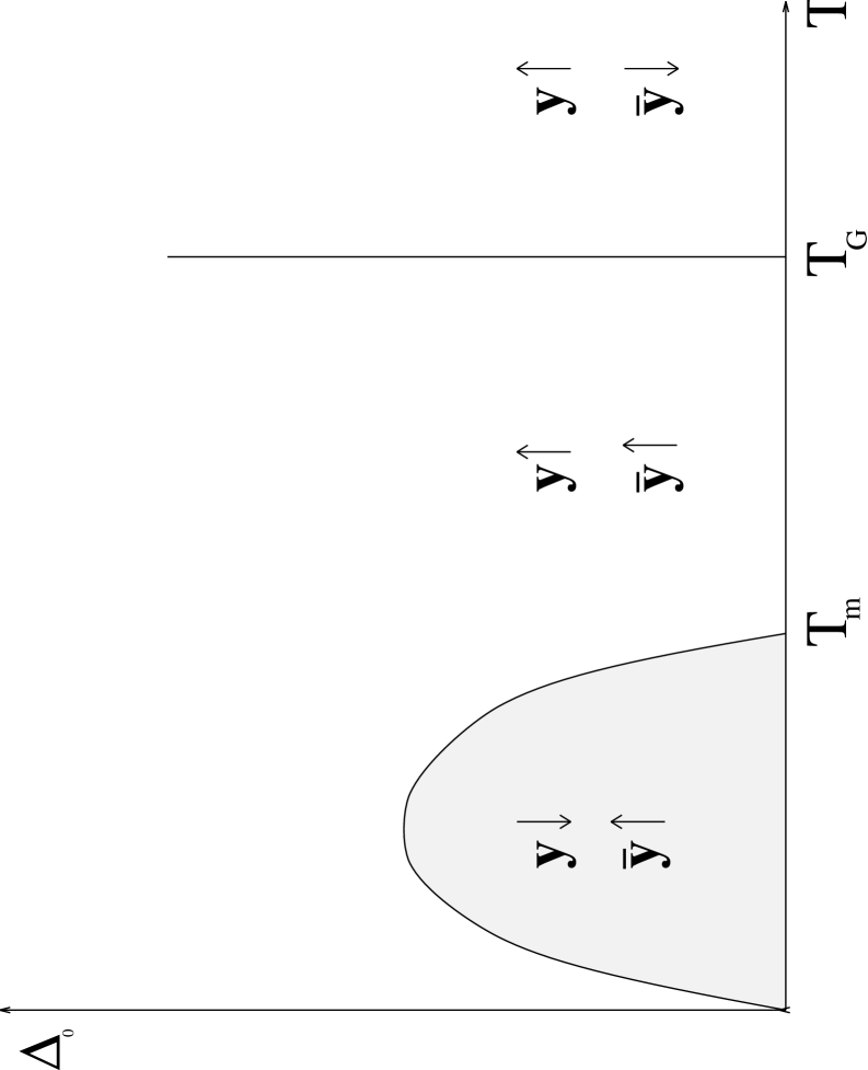
FIG. 5.: Stability diagram of a two dimensional solid with weak quenched substrate disorder, as a function of the temperature $T$ and the long wavelength (i.e harmonic) part of the disorder $\Delta_{0}$. The diagram indicates schematically the stability of the harmonic part of the free energy to dislocations (fugacity $y$) and short-wavelength disorder ($\overline{y}\sim\Delta_{K_{0}}$) by showing the relevance of these variables to linear order.

In presence of dislocations there are thus various possible regimes. There are two critical temperatures. One is the KTHNY melting temperature $T_{m}=a^{2}c_{66}(c_{11}-c_{66})/4\pi c_{11}$, above which dislocations unbind for the pure system which melt into a hexatic. The other one is the glass transition temperature $T_{G}=8\pi c_{11}c_{66}/K_{0}^{2}(c_{11}+c_{66})$, below which disorder becomes relevant in the absence of dislocations. The ratio between these temperatures is equal to half of the exponent $\eta_{K_{0}}$ of the pure system at $T_{m}$. For the CO model it is thus universal and equal to $T_{m}/T_{G}=1/8$. For the triangular lattice it depends on the (renormalized) elastic constants [19] but cannot exceed $1/6$. In figure 5 we have shown schematically how $y$ and $\overline{y}\sim\Delta_{K_{0}}$ are renormalized, at linear order as a function of temperature and long wavelength disorder $\Delta_{0}$ from 190 191. At high temperature dislocations are relevant and disorder is washed away by thermal fluctuations. Below $T_{G}$ disorder becomes relevant leading, in the absence of dislocations, to the Cardy-Ostlund line of fixed points. This line however is unstable to dislocations. In the shaded region in figure 5, the dislocations would be perturbatively irrelevant for the system with $\Delta_{K_{0}}=0$ and the solid would survive ( in fact in that case if one includes non linearities in $y$ the solid is stable in an even greater region [54] ). However in this region the disorder $\overline{y}\sim\Delta_{K_{0}}$ is relevant. It will eventually increase $\Delta_{0}$ as can be seen from (180), and drive the flow towards the region where $y$ itself increases and unpaired dislocations will eventually appear at large scale.

Let us now estimate at which scale dislocations will appear, assuming weak disorder. The disorder $\Delta_{K_{0}}=0$ becomes of order one at lengthscale of order $\xi$. The key point is that up to this lengthscale the fugacity of dislocation has been renormalized downwards and is now much smaller with $y(\xi)/y(a)\sim(a/\xi)^{2(1-T_{m}/T)}$. At this lengthscale, one ends up with a system for which the disorder is of order one and the fugacity of dislocations is extremely small. One can therefore predict that the typical distance between unpaired dislocation $\xi_{D}$ in the shaded region is much larger than $\xi$, the distance above which effects of disorder manifest and (175) can be observed. It is impossible to compute rigorously the ratio $\xi_{D}/\xi$ using perturbative RG since beyond $\xi$ one of the coupling constant ($\Delta_{K_{0}}$) is large, but one can still estimate this ratio by the following heuristic argument. If one assumes that, when $\Delta_{K_{0}}$ has become of order one, (180) is still valid, then above length of order $\xi$,

$$\Delta_{0}(l)=\Delta_{0}+\alpha l$$ (192)

where $\alpha$, is a coefficient of order one. Then estimating the distance between dislocations as the scale at which $y$ becomes of order one, one gets using 188

$$\xi_{D}\sim\xi\exp{\left(C\log^{1/2}((\xi/a)^{2(T_{m}/T-1)}/y(a))\right)}$$ (193)

where $C$ is a constant of order unity and $y(a)$ the bare value of the dislocation fugacity.

The resulting prediction is that in the shaded region of figure 5 dislocations appear only at scales large compared to $\xi$, and the main reason for decay of translational correlations is the pinning of the elastic manifold. Thus the elastic theory developped in this paper should apply up to distances up to order $\xi_{D}$. In that low temperature region perturbative RG does not allow to obtain precisely the correlation functions even at not too large distance since one is far from the perturbative region $T\sim T_{G}$. The variational method on the other hand predicts the following results: as shown in appendix E, there is a crossover temperature $T^{*}=T_{G}/\log(\xi/a)$. For temperatures $T>T^{*}$ there is no intermediate random manifold regime and the displacement correlation function should show the logarithmic growth of (175). However since the disordered solid regime corresponds to $T<T_{m}\simeq T_{G}/8$, one is likely to be in the regime $T<T^{*}$. In that case there is a random manifold regime at short distances where the displacement correlation function grows as $\tilde{B}(x)\sim(x/\xi)^{2/3}$. At large distance one recovers the logarithmic asymptotic regime. The anisotropy ratio between the longitudinal and transverse displacements $R=\tilde{B}_{T}/\tilde{B}_{L}$ should crossover from $2\nu+1\simeq 1.7$ in the random manifold regime to $1$ in the asymptotic regime.

Experimentally, in the system of magnetic bubbles [55, 14] some regimes are found indeed where the distance between dislocations $\xi_{D}$ is of the order of up to five times the translational correlation length. The authors of Ref. [14] observe a crossover between a regime where $\xi_{D}\sim\xi$ to a regime where $\xi_{D}\gg\xi$, which probably corresponds to the transition to the shaded region discussed above. Indeed, the measured ratio $\xi_{D}/\xi$ keeps increasing with density and is limited there only by experimental setting. It would be very interesting to increase the range experimentally accessible. In Ref. [14] some comparison with the random manifold result was also performed. However the definition of the anisotropy ratio used in Ref. [14] ($\xi_{T}/\xi_{L}$) does not seem appropriate, since the data were first fitted to a simple Lorentzian shape. New insight in the physics of such disordered 2D systems could be gained by a reanalysis of these data. More theoretical work is also needed since the above analysis of the dislocations is very crude. It has been generally assumed that the non perturbative RG flow in presence of dislocations was towards a kind of hexatic, but nothing is really known on this phase. In particular, in the Cardy-Ostlund approach, the vortices are supposed to be completely thermalized and to see only a uniform potential, and feel no effect of the disorder. This is physically incorrect, since in a disordered system the fugacity will also depend on the position. One should therefore take also into account terms which will pin the vortices. This is another reason why we believe that the CO analysis overestimates the effect of topological defects.

To conclude, $d=2$ elastic disordered systems have therefore a very rich behavior. Many other experimental systems could be investigated, among them colloids [56, 57] and thin superconductors. A realization which would exclude dislocations could be to adsorb a polymerized membrane, with very high dislocation core energy, on a disordered substrate.

VII Conclusion

In this paper we have developed a quantitative description of the static properties of a lattice in presence of weak disorder. We have derived a model (15) valid in the elastic limit $\nabla u\sim a/\xi\ll 1$ which contains the proper physics at all lengthscales, and allows to describe the various regimes as function of distance. We have applied the Gaussian Variational Method (GVM) to this model and computed the correlation functions of the relative displacements. This method has the advantage of being applicable in any dimension. The comparison with the renormalization group study that we have also performed, which is possible in $d=4-\epsilon$ and in $d=2$, indicates that the GVM is an accurate variational ansatz for this problem. It also shows that the GVM should be a good tool to explore other disordered problems where different length scales are present. Contrary to previous studies the present analysis includes both the effect of metastable states and of the intrinsic periodicity of the lattice, both effects being found to be very important.

We found that the effect of impurities on the translational order of the lattice is weaker than was previously thought and that quasi-long range order persists at large scales. The resulting phase, which we call a “Bragg glass” has both the properties of being a glass and of being quasi-ordered. The analogy with the quasi-order which subsist at low temperature in pure two dimensional solids is puzzling. The Bragg glass possess several intrinsic length scales. At very short scales it behaves as predicted by Larkin’s random force model. This regime should be quite limited in $d=3$ at low temperature and for a potential rough at scales smaller than the lattice. In $d=2$ however, thermal effects being stronger, this regime is wider. At intermediate scales, and low temperature in $d=2$, the system behaves as a random manifold of flux lines independently pinned by impurities with stretched exponential decay of translational order. At distances larger than $\xi$, we have shown that due to the periodicity of the lattice, the pinning by impurities becomes less effective and quasi order survives.

We have not attempted to include explicitly topological defects in the present quantitative study. However, we have given evidence both in $d=3$ and $d=2$ that for weak impurity disorder the effects of dislocations is less important than is usually believed. This is due to the fact that quasi-long range order subsists even in the presence of disorder for the elastic system. In $d=2$ it is possible, but by no means established, that unpaired dislocations will appear at large scale. We have estimated conservatively the length scale at which this happens and found that it can be much larger than $\xi$. Thus in $d=2$ there is a regime where the decay of translational order is due primarily to the elastic displacements induced by disorder. In $d=3$, we have argued that there is probably a phase without unpaired dislocations for weak disorder and at low temperature.

Thus in the three-dimensional high temperature superconductors there could be generically be (at least) two types of glass phases caused by point impurities, i.e two types of vortex glasses. The first one is the strong disorder vortex glass phase which is described by the gauge glass type of models [4, 20] and presumably contains a lot of dislocations. The second one is the quasi-ordered Bragg glass described in the present paper. A natural speculation then is that the tricritical point recently observed in experiments [58], whose position in the $H-T$ plane can be raised by adding more point impurities in a controlled fashion [37], has something to do with the relevance of dislocations. It could mark the separation between these two phases since it is natural that the quasi-ordered glass melts through a sharper transition [59], much like a pure solid, while the vortex glass transition of Ref. [4, 20] is believed to be continuous. [4, 20] In fact, it is not even clear whether, strictly speaking, the strongly disordered vortex glass phase of Ref. [4, 20] is a true thermodynamic phase, rather than a very long crossover from the flux liquid. Indeed recent simulations indicate that $d=3$ could be slightly below its the lower critical dimension [21]. The Bragg glass, on the other hand, should not suffer from such existential problems.

The results of the present study suggest some comments concerning experiments. First decoration experiments should be reanalyzed. Clearly a fit to a simple exponential as inspired by Ref. [30, 60] is certainly inadequate for pictures where no dislocation is present. Since we predict that the crossover to the asymptotic quasi-ordered regime occurs when the correlation function $C_{K_{0}}(r)$ is of order $0.1$ this crossover should be observable, in principle. One must keep in mind that Abrikosov lattices might not be the ideal system to compare with the theory, since they are very complicated objects with additional intrinsic scales. In particular the effect of nonlocal elasticity, 2d to 3d crossover effects and surface interactions, although they can in principle be incorporated into the method, complicate the analysis by introducing new crossover lengths such as the London length. It would be therefore highly desirable, in order to test the above predictions to investigate simpler elastic systems. One example are colloids which have been very successful to investigate translational order in pure systems [56, 57]. In addition, these experiments could help decide whether dislocations are a thermodynamic property of the state or simply a non equilibrium feature which can be eliminated. Neutron diffraction experiments could also help decide on these issues. We obtained several characteristic predictions for neutron diffraction, such as the existence of algebraically diverging Bragg peaks and predictions for the ratio of transverse to longitudinal scattering intensities.

We have addressed here only the statics of a lattice in presence of disorder, the quantities of interest in that case being mainly related to positional order. It would be clearly very interesting to obtain information on the dynamics and especially the driven dynamics of such systems. This is indeed particularly important for superconductors where most experiments measure only dynamical quantities. Several remarks are in order.

There exist presently a qualitative approach to the dynamics of the vortex glass based mostly on scaling arguments for energy barriers [3]. On such a qualitative level one usually assumes a single scale for the energy landscape, i.e that barriers $E_{b}(L)\sim L^{\theta}$ scale with the same exponent $\theta$ which describes energy fluctuations in the statics. Assuming that there is a regime of transport where plastic deformations can be neglected, i.e that energy barriers are controlled only by elastic motion, the present study of the statics can be used to describe the creep regime at low temperature. The argument goes that in presence of an applied external force $f$, such as the Lorentz force created by an external current $|f|\sim|j|$, the barrier for an optimal deformation $u\sim L^{\nu}$ away from a low energy configuration on a scale $L$ is lowered and becomes $E_{b}(L)\sim L^{\theta}-fuL^{d}$. To unpin locally the manifold thus needs to go over an Arrhenius barrier $E_{b}\sim 1/f^{\mu}$ with $\mu=\theta/(d+\nu-\theta)$. This, and the exponents found here lead to a non linear voltage-current relation $V\sim\exp[-1/(Tj^{\mu})]$ in the flux creep regime, where $\mu$ crosses over from $\mu\approx 0.7-0.8$ to $\mu=1/2$ as $j$ decreases.

On a more fundamental level one anticipates that the methods used here for the statics and the results they yielded will set the ground for the study of the dynamics. As was discovered recently [61] the hierarchical structure of states which is encoded in the replica symmetry breaking solution of the statics finds an exact translation in the dynamics. There it corresponds to the existence of a long time dynamics for which the fluctuation dissipation theorem breaks down and non equal time correlation and response functions become highly non trivial. It would be interesting to generalize these studies to the flux lattice. Let us finally note that the quantities computed here using the statics are equal time disorder-averages and they will coincide with the observed translational averages in a given experiment provided equilibrium has been reached, which will always hold below a certain length scale.

We thank D.J. Bishop, J.P. Bouchaud, M. Charalambous, D. Fisher, M. Gabay, D. Huse, T. Hwa, M. Mezard, C.M. Murray, R. Sheshadri. for interesting discussions

A Relabeling of the lines

In this appendix we detail the derivation of expression (9) for the decomposition of the density in term of the relabeling field (8). We denote $d$-dimensional positions $x=(r,z)$ where $r$ belongs to the $m$-dimensional transverse space. The density is given by (3)

$$\rho(x)=\sum_{i}\delta(r-R_{i}-u_{i}(z))$$ (A1)

In order to take the continuum limit, one can introduce a smooth displacement field $u(r,z)$ by

$$u(r,z)=\int_{BZ}\frac{d^{d}m}{(2\pi)^{m}}e^{iq_{\perp}r}\sum_{j}e^{-iq_{\perp}R_{j}}u_{j}(z)$$ (A2)

such that $u(R_{i},z)=u_{i}(z)$ which has no Fourier components outside of the Brillouin zone (BZ). In terms of the smooth field (A2) one can introduce the relabeling field

$$\phi(r,z)=r-u(\phi(r,z),z)$$ (A3)

In the absence of dislocations there is a unique solution of (A3) giving $u(r,z)$ as a function of $\phi(r,z)$. $\phi$ is a m-component smooth vector field labeling the lines, and which takes an integer-like values at each location of a line

$$\phi(R_{i}+u(R_{i},z),z)=R_{i}$$ (A4)

Substituting (A3) in (A1) one gets

$$\rho(x)=\sum_{i}\delta(R_{i}-\phi(r,z))\text{det}[\partial_{\alpha}\phi_{\beta}(r,z)]$$ (A5)

Using the integral representation of the $\delta$ function, (A5) becomes

$$\rho(x)=\text{det}[\partial_{\alpha}\phi_{\beta}]\int\frac{d^{d}q}{(2\pi)^{d}}\rho_{0}(q)e^{iq\phi(x)}$$ (A6)

where

$$\rho_{0}(q)=\sum_{i}e^{iqR_{i}}$$ (A7)

For the case of a perfect lattice $\rho_{0}(q)$ is

$$\rho_{0}(q)=\rho_{0}(2\pi)^{d}\sum_{K}\delta(q-K)$$ (A8)

Using (A8) in (A6) one gets formula (9).

$$\rho(x)=\rho_{0}\text{det}[\partial_{\alpha}\phi_{\beta}]\sum_{K}e^{i{K}\cdot\phi(x)}$$ (A9)

Assuming that we are in the elastic limit $\partial_{\alpha}u_{\beta}\ll 1$ one can expand (A9) to get

$$\rho(x)\simeq\rho_{0}[1-\partial_{\alpha}u_{\alpha}(\phi(x))+\sum_{K\neq 0}e^{iK(r-u(\phi(x),z))}]$$ (A10)

In (A10) one can replace $u(\phi(r,z),z)$ by $u(r,z)$ up to terms of order $\partial_{\alpha}u_{\beta}\ll 1$. Note that in doing so $u$ has negligible (suppressed by powers of $a/\xi$) Fourier components outside the Brillouin zone, and thus there is a complete decoupling between the gradient term and higher $K$ terms.

The same procedure can be carried on in the case where the equilibrium lattice of the $R_{i}$ contains topological defects such as dislocations, vacancies etc. Suppose for instance that one wants to study a lattice with a fixed number of dislocations at prescribed positions in the internal coordinate of the lattice, i.e a network with a fixed topology (connectivity), but which is now allowed to fluctuate in the embedding space due to coupling to disorder and thermal noise. This is relevant for the physical situation of a flux lattice with quenched-in dislocations whenever one can neglect dislocation motion, i.e glide and climb. The equilibrium positions $R_{i}$ now correspond to a minimum of the elastic energy with the constraint of prescribed connectivity. The problem at hand is to analyze the extra small elastic displacements around the equilibrium position due to disorder. The density is still given by (A6) where $\rho_{0}(q)$ is now the Fourier transform of the lattice of the $R_{i}$ (A7).

Upon coupling to disorder, the equivalent of the last term in (15) will be generated. After averaging over the random potential it reads:

$$\int\frac{d^{d}q}{(2\pi)^{d}}\frac{\Delta_{q}}{2T}\cos(q(u^{a}(x)-u^{b}(x)))S(q)$$ (A11)

where $S(q)=\rho_{0}(q)\rho_{0}(-q)$ (with no averages) is the structure factor of the lattice without disorder, with fixed connectivity and in its equilibrium position. If in addition one wants to allow for topological defects to equilibrate one needs to perform some further average over connectivities, which is a difficult task.

B Link with quantum models in $1+1$ dimensions

The variational method can also be applied to study disordered one dimensional (space) interacting bosons or fermions. To see that fact we use a representation of operators in terms of phase fields introduced by Haldane [34]. This representation maps the system into an elastic hamiltonian similar to the one used to describe flux lattices in II.

The single-particle creation operator is written:

$$\Psi^{\dagger}(x)=[\rho(x)]^{\frac{1}{2}}e^{i\theta(x)}$$ (B1)

where $\rho(x)$ is the particle density operator and $\theta(x)$ the phase of the $\Psi$ field. To take into account the discrete nature of the particle density, one introduces an operator $\Phi$ which increases by $\pi$ at each particle’s location. The density operator then is

$$\rho(x)=\frac{1}{\pi}\frac{\partial\Phi(x)}{\partial x}\sum_{m=-\infty}^{+\infty}\exp[2im\Phi(x)]$$ (B2)

$\Phi$ can be expressed in term of another operator $\phi$ by $\Phi=\pi\rho_{0}x+\phi$, and $\rho_{0}$ is the average density. The $\phi$ and $\theta$ fields obey the canonical commutation relations

$$[\phi(x),\frac{1}{\pi}\theta(x^{\prime})]=i\delta(x-x^{\prime})$$ (B3)

Using (B1), the single particle operator becomes[34]

$$\Psi^{\dagger}(x)=[\rho_{0}+\frac{1}{\pi}\nabla\phi(x)]^{1/2}\sum_{m}e^{im(\pi\rho_{0}x+\phi(x))}e^{i\theta(x)}$$ (B4)

For fermions the sum over $m$ in (B4) is only over odd $m$, whereas for boson the sum is only over even values of $m$. For fermions $\pi\rho_{0}$ can be replaced in (B4) by $k_{F}$, where $k_{F}$ is the Fermi momentum. The long-wavelength – low-energy properties of the interacting boson or fermion gas are described by the Hamiltonian [34]:

$$H=\frac{1}{2\pi}\int dx\,\{(\frac{v}{K})(\partial_{x}\phi)^{2}+(vK)(\partial_{x}\theta)^{2}\}$$ (B5)

When going to the Lagrangian, one gets

$${\cal L}=\frac{1}{2\pi K}\int dxd\tau[\frac{1}{u}(\partial_{\tau}\phi)^{2}+u(\partial_{x}\phi)^{2}]$$ (B6)

which is obviously the same than the classical Hamiltonian (2).

From Galilean invariance one has $(vK)/\pi=\rho_{0}/m$, and $v^{2}=1/(\kappa\rho_{0}m)$, where $\kappa$ is the compressibility. $v$ and $K$ are therefore functions of the interactions and incorporate all the interaction effects. The excited states of $H$ are sound waves with phase velocity $v$. For the fermion problem the noninteracting case corresponds to $v=v_{F}$ and $K=1$. For repulsive interactions $K<1$, whereas $K>1$ for attractive ones. For the boson problem $K\to\infty$ when the repulsion between bosons goes to zero, and $K$ decreases for increasing repulsive interactions. For the case of a $\delta$ function repulsion, $K$ varies from $\infty$ to $1$. $K=1$ would correspond to an infinite on site repulsion. $K<1$ can be obtained only if longer range interactions are considered. The coefficient $K$ determines the asymptotic behavior of the correlation functions[34]. For the bosons one gets

$$\begin{array}[]{lcl}\langle\Psi^{\dagger}_{B}(r)\Psi_{B}(0)\rangle&=&B\rho_{0}(\rho_{0}r)^{-1/(2K_{b})}\\ \langle\rho(r)\rho(0)\rangle&=&2K_{b}(2\pi\rho_{0}r)^{-2}+A\rho_{0}^{2}(\rho_{0}r)^{-2K_{b}}\cos(2\pi\rho_{0}r)\end{array}$$ (B7)

with some numerical constants $A$ and $B$. whereas the fermion correlation functions are

$$\begin{array}[]{lcl}\langle\Psi^{\dagger}_{F}(r)\Psi_{F}(0)\rangle&=&B\rho_{0}(\rho_{0}r)^{-(K_{f}+K_{f}^{-1})/2}e^{i\pi\rho_{0}r}\\ \langle\rho(r)\rho(0)\rangle&=&2K_{f}(2\pi\rho_{0}r)^{-2}+A\rho_{0}^{2}(\rho_{0}r)^{-2K_{f}}\cos(2k_{F}r)\end{array}$$ (B8)

up to an angular part. The coupling to a random potential uncorrelated in space and time will give again a Lagrangian identical to (15). Terms of the form

$${\cal L}_{\text{dis}}=\sum_{p}\sum_{a\neq b}\int dxd\tau D_{p}\cos(2p(\phi^{a}(x,\tau)-\phi^{b}(x,\tau)))$$ (B9)

where $p$ is an integer and $D_{p}$ some constants proportional to the disorder will appear. They correspond to Fourier components of the random potential close to $2\pi p\rho_{0}$. The Fourier components close to $q=0$ correspond to forward scattering and give terms similar to the gradient terms in (15).

As discussed in Section VI space and time uncorrelated disorder is relevant when $K\leq 1$. The transition point $K=1$ corresponds to non-interacting fermions or equivalently to bosons interacting with infinite $\delta$ repulsive potential. Disorder is thus always relevant for fermions with repulsive interactions, and always irrelevant for fermions with attractive interactions. Disorder is irrelevant for bosons with only finite $delta$-function repulsion, while it becomes relevant for bosons with sufficiently strong longer range interactions. One experimental realization corresponds to flux lines in superconductors, confined to a plane, which can be realized by proper alignement of the magnetic field. It was argued in Ref [53] that this always lead to a glass phase, i.e $K<1$. This does not seem correct to us. If the vortex line interaction was the sum of an infinite repulsive delta (i.e forbidden crossings) and an extra repulsive interaction of finite range $\lambda$, then disorder would indeed always be relevant. But this is not the case, and the on-site interaction is finite, which presumably leaves room for both a glass phase ($K<1$)and a high temperature phase ($K>1$) in this experimental system.

C One-step solution for $d\leq 2$

In this section we examine a one step replica symmetry broken solution. For simplicity we look at the model with a single harmonic (39) We now search a one step symmetry breaking solution of the form

$$\sigma(v) = \sigma_{0}\qquad[\sigma](v)=0\qquad v<v_{c}$$ (C1)

$$\sigma(v) = \sigma_{1}\qquad[\sigma](v)=v_{c}(\sigma_{1}-\sigma_{0})=\Sigma_{1}\qquad v>v_{c}$$ (C2)

With the form (C1) one gets

$$\tilde{G}(q) = \frac{G_{c}(q)}{v_{c}}+(1-\frac{1}{v_{c}})\frac{1}{G_{c}^{-1}(q)+\Sigma_{1}}+\sigma_{0}G_{c}^{2}(q)$$ (C3)

$$G(q,v) = \frac{\Sigma_{1}G_{c}(q)}{v_{c}(G_{c}^{-1}(q)+\Sigma_{1})}+\sigma_{0}G_{c}^{2}(q)\qquad v>v_{c}$$ (C4)

$$G(q,v) = \sigma_{0}G_{c}^{2}(q)\qquad v<v_{c}$$ (C5)

$$\ [G] = 0\qquad v<v_{c}$$ (C6)

$$\ [G] = \frac{\Sigma_{1}G_{c}(q)}{(G_{c}^{-1}(q)+\Sigma_{1})}\qquad v>v_{c}$$ (C7)

To determine $v_{c}$ one has to minimize the free energy

$$F/(nm\Omega) = \frac{T}{2}\int\frac{d^{d}q}{(2\pi)^{d}}\biggl{[}cq^{2}\tilde{G}(q)-\log(G_{c}(q))$$ (C10)

$$-\frac{G(q,0)}{G_{c}(q)}+\int_{0}^{1}\frac{dv}{v^{2}}\log\left[\frac{G_{c}(q)-[G]}{G_{c}(q)}\right]\biggr{]}$$

$$+\frac{\Delta}{2mT}\int_{0}^{1}dve^{-\frac{K_{0}^{2}}{2}B(0,v)}$$

where

$$B(0,v) = 2T\int\frac{d^{d}q}{(2\pi)^{d}}\frac{1}{G_{c}^{-1}(q)+\Sigma_{1}}\qquad v\geq v_{c}$$ (C11)

$$B(0,v) = B(0,v\geq v_{c})+2T\int\frac{d^{d}q}{(2\pi)^{d}}\frac{\Sigma_{1}}{G_{c}^{-1}(q)(G_{c}^{-1}(q)+\Sigma_{1})v_{c}}\qquad v<v_{c}$$ (C12)

To get the saddle point equations one has to differentiate (C10) with respect to $\sigma_{0}(q)$, $G_{c}$, $\Sigma_{1}$ and $v_{c}$. Differentiation with respect of $\sigma_{0}(q)$ gives $G_{c}^{-1}(q)=cq^{2}$. Differentiating with respect of $1/v_{c}$ and $\Sigma_{1}$ and then replacing $G_{c}^{-1}(q)$ by its value one gets

$$\Sigma_{1} = \frac{K_{0}^{2}\Delta v_{c}}{mT}e^{-K_{0}^{2}T\int\frac{d^{d}q}{(2\pi)^{d}}\frac{1}{cq^{2}+\Sigma_{1}}}$$ (C13)

$$\Sigma_{1}v_{c} = TK_{0}^{2}\int\frac{d^{d}q}{(2\pi)^{d}}\left[\log(1+\frac{\Sigma_{1}}{cq^{2}})-\frac{\Sigma_{1}}{cq^{2}+\Sigma_{1}}\right]$$ (C14)

Note that $\sigma_{0}$ does not appear in these equations. One could in principle determine the value of $\sigma_{0}$ by differentiating (C10) with respect to $G_{c}^{-1}(q)$. However it is much easier to use the saddle point equations (37). For $d\leq 2$ one has

$$\sigma_{1} = K_{0}^{2}\frac{\Delta}{mT}e^{-K_{0}^{2}T\int\frac{d^{d}q}{(2\pi)^{d}}\frac{1}{cq^{2}+\Sigma_{1}}}$$ (C15)

$$\sigma_{0} = \sigma_{1}e^{-K_{0}^{2}T\int\frac{d^{d}q}{(2\pi)^{d}}\frac{\Sigma_{1}}{cq^{2}(cq^{2}+\Sigma_{1})v_{c}}}$$ (C16)

Thus $\sigma_{0}=0$ for $d\leq 2$. Note that in order to determine $v_{c}$ one should not substitute in (C10) the expressions (C15) before differentiating with respect to $\Sigma_{1}$ and $1/v_{c}$. Such expressions are only valid at the saddle point.

In $d=2$ the above equations read:

$$\Sigma_{1}v_{c} = TK_{0}^{2}\frac{\Lambda}{4\pi c}\log[1+\frac{\Sigma_{1}}{\Lambda}]$$ (C17)

$$\Sigma_{1} = K_{0}^{2}\frac{\Delta v_{c}}{mT}\left(\frac{\Lambda}{\Sigma_{1}}+1\right)^{-K_{0}^{2}T/(4\pi c)}$$ (C18)

where we used a circular cutoff $\Lambda\simeq c(2\pi/a)^{2}$. Let us denote by $T_{c}=4\pi c/K_{0}^{2}$ and $y=\Sigma_{1}/\Lambda$. We then have:

$$v_{c} = \frac{T}{T_{c}}\frac{\log(1+y)}{y}$$ (C19)

$$y^{(1-T/T_{c})} = \frac{K_{0}^{2}\Delta}{mT_{c}\Lambda}\frac{\log[1+y]}{y(1+y)^{T/T_{c}}}$$ (C20)

We are interested in the case $\frac{K_{0}^{2}\Delta}{mT_{c}\Lambda}<1$ since $\xi\gg a$ and thus there is clearly a one step solution for $T<T_{c}$. Note that for arbitrary $\Lambda$ $\Sigma_{1}$ vanishes when $T\to T_{c}^{-}$ and simultaneously $v_{c}$ goes to $1$.

For $d<2$ the above equations lead to

$$v_{c} = TK_{0}^{2}(\frac{2-d}{d})j_{d}\Sigma_{1}^{\frac{d-2}{2}}c^{-d/2}$$ (C21)

$$\ \Sigma_{1} = \frac{K_{0}^{2}\Delta v_{c}}{mT}e^{-K_{0}^{2}Tj_{d}\Sigma_{1}^{(d-2)/2}c^{-d/2}}$$ (C22)

where

$$j_{d}=\int\frac{d^{d}q}{(2\pi)^{d}}\frac{1}{q^{2}+1}=\frac{\pi^{1-d/2}}{2^{d}\sin(\pi d/2)\Gamma[d/2]}$$ (C23)

We can compare the free energy (C10) of the one step solution with the free energy of the symmetric one, that one obtains by taking $v_{c}=1$ and $\Sigma_{1}=0$. The free energy difference $\Delta F=F_{\text{onestep}}-F_{\text{rs}}$ is

$$\frac{\Delta F}{mn\Omega}=\frac{T}{2}(\frac{1}{v_{c}}-1)\int\frac{d^{d}q}{(2\pi)^{d}}\left[\frac{\Sigma_{1}}{cq^{2}+\Sigma_{1}}-\log(\frac{cq^{2}+\Sigma_{1}}{cq^{2}})\right]+(1-v_{c})\frac{\Delta}{2mT}e^{-K_{0}^{2}B(0,v_{c})/2}$$ (C24)

where $B(0,v_{c})$ is obtained from (C11). Using the saddle point equations (C13), (C24) simplifies into

$$\frac{\Delta F}{mn\Omega}=\frac{\Sigma_{1}}{2K_{0}^{2}}\frac{(1-v_{c})^{2}}{v_{c}}$$ (C25)

Thus whenever there exist a one step solution it has higher energy than the replica symmetric solution.

Examining the equations C21 one sees that indeed a one step solution survives in $d=1$ even while the replica symmetric solution is stable there. Note however that the one step solution changes nature and, as an approximation to the original problem, acquire some unphysical features. In $d=1$ it does not exist for small disorder at fixed $T$. When it exist the transition is discontinuous and $\Sigma_{1}$ jumps from zero to some non zero value. The equations are in fact very similar to a variational approach to roughening in $d=1$ where it is obvious that the cosine term is irrelevant and the variational approach cannot be trusted beyond weak disorder, where it gives sensible results. Here it is also clear that $q=K_{0}$ disorder (i.e the cosine term) is irrelevant at large scale for $d<2$, in the sense that it will not pin the $d=1$ manifold. It will however renormalize the long-wavelength disorder which simply adds to the thermal roughening $u\sim L^{1/2}$. The physical meaning of the one step solution for $d=1$ being unclear, although it could be related to transitions in the dynamics, we will not considering further. Note finally that in $d=0$ the one step solution does not exist at all ( since the mass is zero).

D Variational calculation on the non-local model

If one does not use the decomposition (10) of the density, the variational equation for the off diagonal self energy is [26, 25] instead of (29) (in the presence of the extra disorder (104))

$$\sigma_{a\neq b}(q_{\perp})=\frac{\Delta}{T}\sum_{i}\frac{1}{R_{i}^{\lambda}}\frac{1}{B_{ab}^{m/2+1}(R_{i})}(\frac{m}{2}-\frac{R_{i}^{2}}{2B_{ab}(R_{i})})e^{-\frac{R_{i}^{2}}{2B_{ab}(R_{i})}}\cos(q_{\perp}R_{i})$$ (D1)

As for the local model (15) one has to look for a non replica symmetric solution. Let us use the Poisson formula valid for arbitrary lattice of $R_{i}$:

$$vol(R_{i})\sum_{R_{i}}\delta(x-R_{i})=\sum_{K}e^{iKx}$$ (D2)

where $vol(R_{i})$ is the volume of the unit cell and the $K$ are the reciprocal lattice vectors. One can then replace the discrete sum in (D1) by an integral and insert the integration over $x$ in formula (D1). One gets

$$\sigma(q_{\perp},v)=\frac{\rho_{0}\Delta}{T}\sum_{K}\int d^{m}re^{iKr}\frac{1}{r^{\lambda}}\frac{1}{B^{m/2+1}(r,v)}(\frac{m}{2}-\frac{r^{2}}{2B(r,v)})e^{-\frac{r^{2}}{2B(r,v)}}\cos(q_{\perp}r)$$ (D3)

From this exact expression, BMY kept only the components with $K=0$. As pointed out by BMY, [26, 25] if one takes $v$ small enough, then $B(r=1,v)$ is large enough so that, for all the $r$ contributing to (D3), one can replace $B(r,v)$ by $B(0,v)$. The idea is that $B(r,v)$ varies much more slowly that $r^{2}$, which is true in the elastic limit. Indeed one can easily see that for small $v$ and large $r$ one has $B(r,v)\propto\log(v_{\xi}/v)+C\log(r)$. Thus $B(r,v)\simeq r^{2}$ implies that $r\sim\log(v_{\xi}/v)^{1/2}$, and therefore $B(r,v)\simeq B(0,v)$. If one does so and since $B(0,v)\gg 1$, one can restrict oneself to $K=0$ or $K=\pm K_{0}$ in (D3). The off diagonal part of the self energy becomes

$$\sigma(q,v)\simeq\lambda B(0,v)^{-1-\lambda/2}+c_{1}q^{2}e^{-\frac{q^{2}}{2}B(0,v)}+c_{2}e^{-\frac{K_{0}^{2}}{2}B(0,v)}$$ (D4)

The two first terms in (D4) come from the $K=0$ part in (D3). The term in $\lambda$ is due to the extra unphysical disorder and, as long as $\lambda$ is finite dominates the long range behavior ($q\to 0$ and large $B(0,v)$). The other terms correspond to the same separation of the Fourier components of the random potential than in the discussion leading to our model (15). The $q\simeq 0$ components gives the same contribution than the terms in (15) in $\nabla u_{a}\nabla u_{b}$. Indeed this $K=0$ term comes from

$$\langle\int drdr^{\prime}\delta(r-r^{\prime}+u^{a}(r)-u^{b}(r^{\prime}))\rangle$$ (D5)

This term measures the smooth change in local density due to the slowly varying displacement field, and keeping only this term amounts to neglect the discreteness of the vortices in the original Hamiltonian. The third term in (D4) comes from the $q\simeq K_{0}$ component of the disorder, i.e. the part which has the periodicity of the equilibrium lattice. For the physical disorder $\lambda=0$ (D4) is identical to the one obtained from the local model (15).

In fact neglecting the $x$ dependence in $B(x,v)$ is equivalent to the replacement $\phi(x)=x-u(x)$, i.e identifying $u(\phi(x))-u(\phi(y))$ with $u(x)-u(y)$, which led to the model (15). Such a replacement becomes exact in the elastic limit $\overline{\langle(\nabla u)^{2}\rangle}\ll 1$ which has been checked self consistently on our solution.

E Random manifold in $d=2$

Let us consider the original model (15) in $d=2$ keeping all the harmonics. We will treat only the simpler case of isotropic elastic matrix, but for arbitrary $m$ and lattice symmetry. Similarly to the study in $d>2$ we use the rescaled quantities (55) which satisfy the rescaled equations (67). In $d=2$ one has $\xi=a^{2}c\sqrt{m/4\pi^{3}\Delta_{K_{0}}}$ and $v_{\xi}=\pi T/a^{2}c$. The equations read:

$$[s](y) = h(z)$$ (E1)

$$y = -h^{\prime}(z)/h(z)$$ (E2)

where $h(z)$ is defined in (61). It appears clearly on (E2) that $y$ has a minimum value which is

$$y_{0}=\left(\frac{K_{0}a}{2\pi}\right)^{2}$$ (E3)

Thus the function $[\sigma](v)$ must vanish for $v<v_{0}=v_{\xi}y_{0}=T/T_{c}$ which is identical to the value of the breakpoint $v_{c}$ in (168) of the one step solution for the single cosine model. The asymptotic behavior at large distance will thus be identical to the one of the single cosine model studied in section III C 1. The transition temperature also turns out to be exactly the same $T_{c}=4\pi c/{K_{0}}^{2}$. However, for $y>y_{0}$, $[s](y)$ will increase continuously until the breakpoint $y=y_{c}$ above which it becomes constant again. Using equation (50) the breakpoint $z_{c}=b(y_{c})$ satisfies

$$z_{c}=\frac{\pi T}{ca^{2}}\log[1+\frac{\Lambda^{2}\xi^{2}}{[s](y_{c})}]$$ (E4)

where we used the circular cutoff $\Lambda=2\pi/a$. Using the equation (E2) one sees that $z_{c}$ is determined as the solution of the equation $z_{c}=f(z_{c})$ where we have defined the function $f(z)$ as:

$$f(z)=\frac{\pi T}{ca^{2}}\log[1+\frac{\Lambda^{2}\xi^{2}}{h(z)}]$$ (E5)

Let us study the function $f(z)$. Using the two limiting forms for $h(z)$, i.e

$$h(z) = Ae^{-\alpha z}~{}~{}~{}z>>1$$ (E6)

$$h(z) = B/z^{(m+4)/2}~{}~{}~{}z<<1$$ (E7)

from 69 and 73, one finds that the function $f(z)$ has three different behaviours depending on the values of $z$

$$f(z) \simeq \frac{\pi T}{ca^{2}}(\alpha z+\log((\xi/a)^{2}/A))\qquad z\gg 1$$ (E8)

$$f(z) \simeq \frac{\pi T}{ca^{2}}(\frac{m+4}{2}\log(z)+\log((\xi/a)^{2}/B))\qquad(a/\xi)^{4/(m+4)}\ll z\ll 1$$ (E9)

$$f(z) \simeq \frac{\pi T}{Bca^{2}}(\xi/a)^{2}z^{(m+4)/2}\qquad z\ll(a/\xi)^{4/(m+4)}$$ (E10)

taking into account that $\xi/a>>1$.

The first regime corresponds to high temperatures. One finds no solution when $T>T_{c}$ and when $T<T_{c}$ one finds $z_{c}=\pi T\log((\xi/a)^{2}/A)/ca^{2}(1-T/T_{c})$. In that regime $y_{c}$ and $y_{0}$ are very close to each other and the solution is very similar to the one step solution of the single cosine model. There is no true random manifold regime.

Solving the equation in the second regime one finds approximately

$$z_{c}\simeq\frac{\pi T}{ca^{2}}\log((\xi/a)^{2}/B){}~{}~{}~{}~{}v_{c}\simeq\ \frac{m+4}{2\log((\xi/a)^{2}/B)}$$ (E11)

where we have used that in that regime $y\simeq(m+4)/(2z)$. The condition $z_{c}\ll 1$ shows that this regime exists only at low temperature:

$$T<T^{*}=\frac{ca^{2}}{\pi\log((\xi/a)^{2}/B)}$$ (E12)

There all the harmonics contribute, $y_{c}$ and $y_{0}$ are very different from each other and there is a large random manifold regime, between the Larkin regime and the asymptotic regime. In this regime one has $\tilde{B}(x)\sim A(x/\xi)^{2\nu}$ with $\nu=\nu_{RM}=2/(4+m)$.

It is easy to see that the last regime of behaviour of $f(z)$ never contributes. This is because one is restricted to values of $z$ such that $v_{c}=y_{c}v_{\xi}<1$ which corresponds to $z_{c}>ca^{2}/(T\pi)$. This regime where there is no breakpoint ($l\sim a$), and therefore no Larkin regime, as already discussed after formula (87), arises at very low temperatures $T<T^{\prime*}\sim(ca^{2}/\pi)(a/\xi)^{4/(4+m)}/\log((\xi/a)^{2}/B)$

REFERENCES

- [1] Laboratoire associé au CNRS. email: giam@lps.u-psud.fr.
- [2] Laboratoire Propre du CNRS, associé a l’Ecole Normale Supérieure et a l’Université Paris-Sud. email: ledou@physique.ens.fr.
- [3] M. Feigelman, V. Geshkenbein, A. Larkin, and V. Vinokur, Phys. Rev. Lett. 63, 2303 (1989).
- [4] M. P. A. Fisher, Phys. Rev. Lett. 62, 1415 (1989).
- [5] D. R. Nelson and V. M. Vinokur, Phys. Rev. B 48, 13060 (1993).
- [6] T. Hwa, P. L. Doussal, D. R. Nelson, and V. M. Vinokur, Phys. Rev. Lett. 71, 3545 (1993).
- [7] For a very recent review see G. Blatter, M. V. Feigel’man, V. B. Geshkenbein, A. I Larkin and V. M. Vinokur, to be published.
- [8] G. Grüner, Rev. Mod. Phys. 60, 1129 (1988).
- [9] E. Y. A. et al., Phys. Rev. Lett. 60, 2765 (1988).
- [10] H. W. J. et al., Phys. Rev. Lett. 65, 633 (1990).
- [11] I. M. Rusin, S. Marianer, and B. I. Shklovskii, Phys. Rev. B 46, 3999 (1992).
- [12] B. G. A. Normand, P. B. Littlewood, and A. J. Millis, Phys. Rev. B 46, 3920 (1992).
- [13] R. Seshadri and R. M. Westervelt, Phys. Rev. B 46, 5142 (1992).
- [14] R. Seshadri and R. M. Westervelt, Phys. Rev. B 46, 5150 (1992).
- [15] V. M. Vinokur and A. E. Koshelev, Sov. Phys. JETP 70, 547 (1990).
- [16] L. Balents and S. H. Simon, Preprint ITP 1994.
- [17] J. Toner and D. DiVincenzo, Phys. Rev. B 41, 632 (1990).
- [18] V. L. Pokrovsky and A. L. Talapov, Phys. Rev. Lett. 42, 65 (1979).
- [19] D. R. Nelson and B. I. Halperin, Phys. Rev. B 19, 2457 (1979).
- [20] D. S. Fisher, M. P. A. Fisher, and D. A. Huse, Phys. Rev. B 43, 130 (1990).
- [21] Bokil and A.P. Young, Absence of a Vortex Glass Transition in a Three-Dimensional Vortex Glass Model with Screening , Preprint 1994.
- [22] T. Giamarchi and P. Le Doussal, in preparation.
- [23] A. Larkin, Sov. Phys. JETP 31, 784 (1970).
- [24] A. I. Larkin and Y. N. Ovchinokov, J. Low Temp. Phys 34, 409 (1979).
- [25] J. Bouchaud, M. Mézard, and J. Yedidia, Phys. Rev. B 46, 14686 (1992).
- [26] J. Bouchaud, M. Mézard, and J. Yedidia, Phys. Rev. Lett. 67, 3840 (1991).
- [27] T. Nattermann, Phys. Rev. Lett. 64, 2454 (1990).
- [28] T. Giamarchi and P. Le Doussal, Phys. Rev. Lett. 72, 1530 (1994).
- [29] M. Mezard and G. Parisi, J. de Phys. I 4, 809 (1991).
- [30] E. Chudnovsky, Phys. Rev. Lett. 65, 3060 (1990).
- [31] D. Grier et al., Phys. Rev. Lett. 66, 2270 (1991).
- [32] U. Yaron et al. “Neutron Diffraction studies of flowing and Pinned Magnetic Flux Lattices in 2H-NbSe2” submitted to Physical Review Letter (1994).
- [33] S. F. Edwards and P. W. Anderson, J. Phys. F 5, 965 (1975).
- [34] F. D. M. Haldane, Phys. Rev. Lett. 47, 1840 (1981).
- [35] H. Fukuyama and P. Lee, Phys. Rev. B 17, 535 (1978).
- [36] S. E. Korshunov, Phys. Rev. B 48, 3969 (1993).
- [37] W. K. Kwok et al., Physica B 197, 579 (1994).
- [38] D. A. Huse, private communication.
- [39] L. I. Glazman and A. E. Koshelev, Phys. Rev. B 43, 2835 (1991).
- [40] D. S. Fisher, in Phenomenology and Applications of High Temperature Superconductors, edited by K. Bedell, M. Inui, D. Metzel,J.R. Schrieffer, and S. Doniach (Addison-Wesley, New York, 1991).
- [41] T. Giamarchi, P. Le Doussal, C.A. Murray, in preparation.
- [42] P. Le Doussal and J. Machta, J. Stat. Phys. 64 541 (1991).
- [43] T. Halpin-Healy, Phys. Rev. A 42, 711 (1990).
- [44] M. C. Marchetti and D. R. Nelson, Phys. Rev. B 47, 12214 (1993).
- [45] P. Le Doussal and T. Giamarchi “Replica symmetry breaking in the 2D XY model in a random magnetic field” to appear in Phys. Rev. Lett. 74 January 1995.
- [46] D. Fisher, Phys. Rev. Lett. 56, 1964 (1986).
- [47] L. Balents and D. S. Fisher, Phys. Rev. B 48, 5959 (1993).
- [48] T. Nattermann and H. Leschhorn, Europhys. Lett. 14, 603 (1991).
- [49] J. Villain and J. Fernandez, Z Phys. B 54, 139 (1984).
- [50] J. Cardy and S. Ostlund, Phys. Rev. B 25, 6899 (1982).
- [51] G. G. Batrouni and T. Hwa, Phys. Rev. Lett. 72, 4133 (1994).
- [52] D. Cule and Y. Shapir, Phys. Rev. Lett. 74, 114 (1995).
- [53] T.Nattermann, I.Lyuksyutov, and M.Schwartz, Europhys. Lett. 16, 295 (1991).
- [54] D. R. Nelson, Phys. Rev. B 27, 2902 (1983).
- [55] R. Seshadri and R. Westervelt, Phys. Rev. Lett. 66, 2774 (1991).
- [56] C. A. Murray, D. H. V. Winkle, and R. Wenk, Phase Transitions 21, 93 (1990).
- [57] C. A. Murray, W. O. Sprenger, and R. Wenk, Phys. Rev. B 42, 688 (1990).
- [58] H. Safar et al., Phys. Rev. Lett. 70, 3800 (1993).
- [59] M. Charalambous, J. Chaussy, and P. Lejay, Phys. Rev. B 45, 5091 (1992).
- [60] E. M. Chudnovsky, Phys. Rev. B 40, 11355 (1989).
- [61] L.F. Cugliandolo and J. Kurchan, J. Phys A 27 5749 (1994).