Amphiphilic membranes

1 Introduction

Amphiphilic molecules (the word derives from the Greek $\alpha\mu\phi\grave{\iota}$ $\phi\iota\lambda\acute{\iota}\alpha$, meaning “love on both sides”) are molecules which both love and hate water. They are formed by two parts with very different tastes, which are covalently bound together: one, the hydrophilic head, is polar or even ionized, and tends therefore to be close to the small, polar water molecules; the other, the hydrophobic tail, is usually a hydrocarbon chain, which perturbs the high order of water, and has therefore the tendency to pack close to similar chains.

Amphiphilic molecules in solvents (water and/or oil) may form several structures (micelles, hexagonal phases, cubic phases…), but we shall discuss mostly the cases in which they form a bilayer, i.e., a sheet made up of two layers of amphiphilic molecules: in water, the hydrophilic heads stem out of the bilayer on both sides, while the corresponding tails remain at the interior. Membranes can be formed by an isolated bilayer or by several bilayers stuck one on top of another: in this case one speaks of multilayers.

Amphiphilic membranes are a physical realization of fluctuating surfaces. They are thin sheets (50–100Å) of amphiphilic molecules immersed in a fluid, usually water or brine (water and salt). They can be of natural or artificial origin: the most important example of natural membranes is the cell membrane, which separates the interior of all living cells from its exterior. Living cells, and in particular eucaryotic ones, possess a large number of membranes, like the nuclear membrane, which separates the nucleus from the rest of the cell, allowing, e.g., mRNA to pass from the inside to the outside, and several chemical signals in the reverse direction, or the Golgi apparatus, which acts as a sort of “chemical factory” for the cell. Mitochondria are also organelles essentially formed by a membrane, folded on itself several times.

Artificial amphiphilic membranes have recently become a lively research field stimulated by their applications in the industry, in medicine and in cosmetics. One can form with them tunable or “active” filters, simulating, as it were, the action of the cell membrane. They are also able to close on themselves, forming vesicles (small closed surfaces), which may act as drug carriers, designed to open up and release their load when the “correct” physico-chemical conditions are found. Several other applications can also be envisaged.

The physics of amphiphilic membranes is a wide subject, and it is out of question to review it fully in this series of lectures. I shall mostly dwell on the aspects which fit more closely the scope of the School, namely those involving shape fluctuations. It will be necessary to review briefly the basic physical chemistry involved to understand why membranes form at all, which features govern their shape, and their equilibrium or dynamical behavior. General introductions to the statistical mechanics of amphiphilic membranes can be found in ref. [93]. A good introduction to the basic properties of biological membranes is found in [114, Chap. 12]. References [109],[21] contain introductions to the physical chemistry of amphiphilic molecules.

Therefore, in the next section I shall briefly dwell on the structure of their basic components, the amphiphilic molecules, and give an overview of the structures they form in the presence of water and/or oil. In the following section I shall discuss the free energy of an isolated fluid membrane as a function of its shape. The corresponding hamiltonian (due to W. Helfrich) lies at the basis of the current understanding of vesicle shapes and of membrane fluctuations. The following section contains a brief review of recent theoretical and experimental work on vesicle shapes. Then the effects of fluctuations on amphiphilic membranes will be discussed: these involve on the one hand the characteristic flicker phenomenon in vesicles, and on the other hand the renormalization of the elastic parameters appearing in the Helfrich hamiltonian. All these aspects are reflected in the phase behavior of interacting fluid membranes to which the last section is dedicated. A few technical points are discussed in the four Appendices.

2 Amphiphilic molecules and the phases they form

Biological membranes are formed by a bilayer of amphiphilic molecules, the most common of which are phospholipids. Their hydrophilic head is a phosphate, and their tail is formed by one or two fatty acids. Most often the two parts are connected by a glycerine hinge, and the molecule is therefore called a phosphoglycerid. The chemical structure of a typical phosphoglycerid is represented in fig. 1.

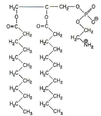
Figure 1: Chemical structure of a typical phosphoglycerid: 1,2 dilauryl-DL-phosphatidylethanolamine (DLPE). From B. L. Silver, The physical chemistry of membranes (Boston: Allen & Unwin, 1988) p. 2.

The glycerine molecule which forms the hinge of the structure is shown on the top. On one side, it is ester-linked to a phosphate group –POOH–O–R carrying the ethanolamine residue R=–CH₂–CH₂–NH₂. In physiological conditions the head is almost always ionized, yielding –PO^-–CH₂–CH₂–NH${}_{3}^{+}$. Via the other two carbons (1 and 2) the glycerine is ester-linked to two fatty acid chains, of the general structure CH₃–(CH₂)_n–COOH. In our case one has $n=10$, and the acid is called acid $n$-dodecanoic, or lauric acid. The example helps to clarify the terminology. Other phosphoglycerids may differ from DLPE either by having just one fatty acid chain (monoglycerids), or by the nature of the fatty acid tail. For example, if the two chains have $n=14$ (palmitic acid) one has dipalmitoylphosphatidylethanolamine, (DPPE). If we change now the residue R to choline R${}_{1}=$–CH₂–CH₂–N⁺–(CH₃)₃, we have dipalmitoylphosphatidylcholine (DPPC), also called lecitin, which is an important component of natural membranes.

In general, the two fatty acids of natural phosphoglycerids are different, and one of them is quite often unsaturated. The knee which appears because of the insaturation, like that shown in fig. 2, helps in keeping the fluidity of the membrane.

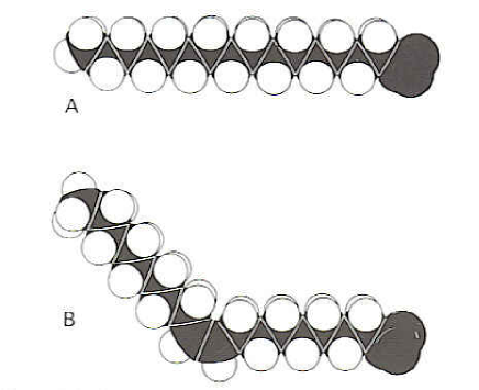
Figure 2: Space filling models of (A) palmitate (C₁₆, saturated) and (B) oleate (C₁₈, unsaturated). The cis double bond in oleate produces a bend in the hydrocarbon chain. From L. Stryer, Biochemistry (New York: Freeman, 1988) p. 285.

Pure phospholipids may be made to crystallize, and the crystal structure of several of them have been determined by X-ray or electron diffraction. In the crystalline state they are stuck in bilayers, their tails all trans, with their heads folded approximately parallel to the bilayer surface and linked (mostly by hydrogen bonds) into a firm network. This organization is schematically represented in fig. 3.

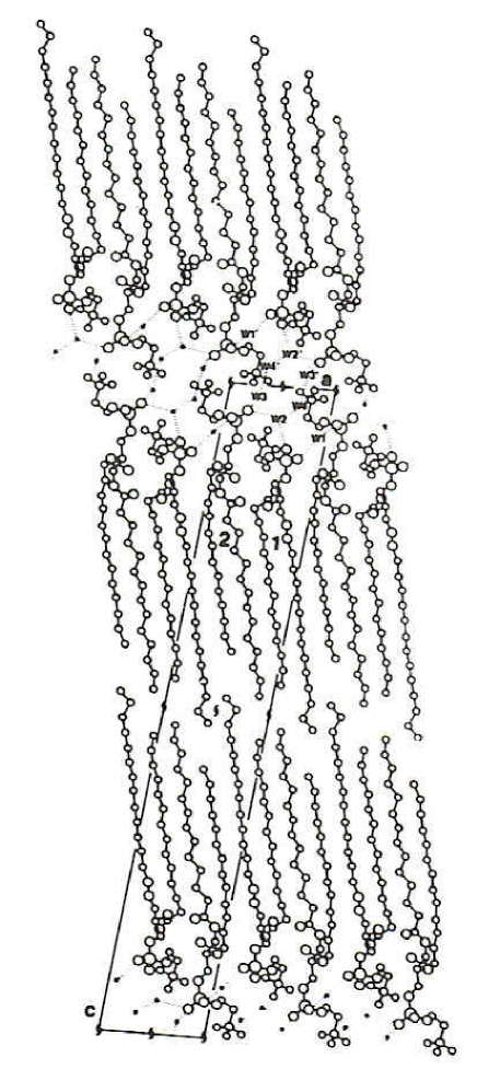
Figure 3: Crystal structure of DMPC projected onto the crystallographic a-c plane. From R. H. Pearson, I. Paschen, Nature 281 499 (1979).

This order is disrupted, as the temperature increases, via a two-step process:

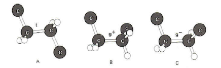
Figure 4: Conformation of C–C bonds in fatty acyl chains: (A) trans (t) conformation; (B and C) a 120^∘ rotation yields a gauche (g) conformation, which can be either g⁺ (clockwise rotation) or g^- (counterclockwise rotation). From L. Stryer, Biochemistry (New York: Freeman, 1988) p. 297.

• At a temperature $T_{\rm t}$ called the transition temperature the order of the chains breaks down: i.e., a significant fraction of the carbon links goes over to the gauche configurations (cf. fig 4), providing a gain in entropy against a loss in van der Waals attraction among the chains. This is sometimes called “chain melting” or “premelting”.

• The actual melting temperature $T_{\rm m}$ is reached when the ionic lattice formed by the hydrophilic heads eventually breaks down.

The melting temperature $T_{\rm m}$ of most pure phosphoglycerids is comparatively high ($\sim 200^{\circ}{\rm C}$), and does not depend strongly on the length of the fatty acid tail. On the other hand the transition temperature is closer to room temperature and increases with the hydrocarbon chain length: a plot is shown in fig. 5.

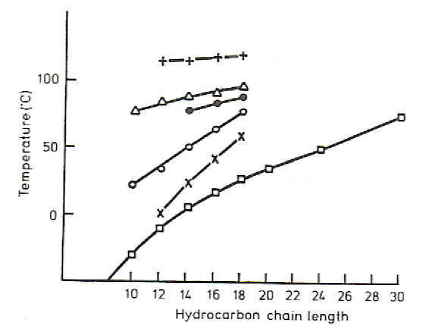
Figure 5: Chain melting temperatures $T_{\rm t}$ for some amphiphiles as a function of chain length. $+$ anhydrous 1,2-diacyl-DL-phosphatidylethanolamines; $\bullet$, 1,2-diacyl-DL-phosphatidylethanolamines in water; $\triangle$, anhydrous 1,2-diacyl-L-phosphatidylcholine monohydrates; $\circ$, 1,2-diacyl-L-phosphatidylcholine monohydrates; $\times$, 1,2-diacyl-L-phosphatidylcholine monohydrates in water. For comparison, the melting points of some normal paraffines, $\Box$, are given. From D. Chapman, et al., Chem. Phys. Lipids 1 445 (1967).

We expect therefore, in most phospholipids, to find a phase in which a relatively fluid hydrocarbon core is sandwiched between two relatively rigid polar sheets. This feature makes possible to sustain fluid bilayers in an aqueous medium. In isolated bilayers in a solvent one observes a sharp anomaly of the specific heat at a transition temperature $T_{\rm t}$ somewhat lower than that observed for pure anhydrous phospholipids (see fig. 6).

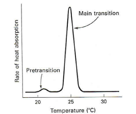
Figure 6: Differential scanning calorimetry of phosphatidyl choline. The small peak (the pretransition) comes from a change in the tilt of fatty acyl chains with respect to the bilayer. The major peak arises from the phase transition in which crystalline fatty acyl chains become disordered because of the introduction of kinks. From L. Stryer, Biochemistry 3rd ed. (New York: Freeman, 1988) p. 297.

This anomaly is accompanied by a fast variation of the mechanical properties of the bilayer, and is known as the “main transition”.

The idea to keep in mind is that amphiphilic molecules are complex ones, with a number of internal degrees of freedom in the tails. The transition takes place essentially in their tails. The disorder in the tails eventually induces a liquid-like disorder in the location of the molecules on the sheet. This is quite different from a melting transition in a sheet of bead-like molecules. The coupling between crystallization and chain ordering has not yet been satisfactorily treated [5]. Its relevance can be grasped from the observation that most biological membranes appear to work very close, but slightly above the transition temperature. Some suggested explanations of this fact can be found in [5].

As soon as water enters the picture, it makes it much more complicated. With a low water content, the system maintains by and large the lamellar organization characteristic of the pure crystal. The layers can exhibit a number of different phases, which have different stability domains. For example in a mixture of dimyristoylphosphatidylcholine (DMPC) and water, one can find at least three phases at high DMPC concentration [67, 46, 47]. They are called the L_α, L_β and P_β phases. In the L_α phase the bilayers are fluid and flat on average. If one lowers the temperature $T$, or decreases the water content $\phi$, one goes to an ordered, “solid like” phase L_β, in which the hydrocarbon chains are ordered and the molecules do not diffuse freely. In these phases, the order of the hydrocarbon chains implies a larger thickness of the bilayers. One can also observe an intermediate “rippled” phase P_β (see fig. 7), in which the bilayers exhibit an undulated structure and almost solid-like diffusion properties [67]. Analysis of X-ray experiments on these “rippled” phases strongly suggests that they are characterized by a modulation of the bilayer thickness [118]. The hydrocarbon chains are often tilted with respect to the bilayer: one then denotes the phases as L${}_{\beta^{\prime}}$ or P${}_{\beta^{\prime}}$. In fact, there are several different L${}_{\beta^{\prime}}$ phases, distinguished by the relationship between the tilt and in-plane bond orientational order [112].

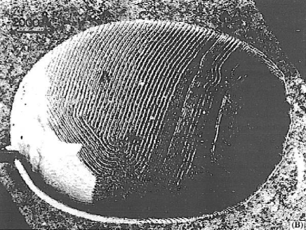
Figure 7: Electron microscope photograph of “rippled” phases in DPPC, produced by cooling large vesicles from the P${}_{\beta^{\prime}}$ phase. From E. Sackmann, et al., Liquid crystals of one- and two-dimensional order, (Berlin: Springer, 1980) p. 314.

The “rippled” P_β phases may be considered as an intermediary structure between the lamellar ones found at low water concentration and the ones found at low amphiphile concentration. If we add amphiphilic molecules to pure water, the molecules first go preferentially to the air-water interface, forming a monolayer, with their heads toward water as long as the concentration does not exceed the critical micelle concentration (cmc), which is of the order of $10^{-10}\,{\rm mol}$. Below the cmc the amphiphilic molecules are overwhelmingly in the monomer form, at higher concentration added monomers appear almost exclusively in aggregates, mainly of globular form with the hydrophilic heads on the surface. These aggregates are called micelles. They form more readily for single-chain amphiphiles (e.g., monoglycerids) and are favored by the presence of large head groups. The structure of micelles is depicted in fig. 8. In this figure, the concentration of amphiphiles is high enough to let the micelles arrange in a close-packed bcc lattice: this is the simplest example of the remarkable cubic phases formed by amphiphiles. As the amphiphile concentration is increased, one observes the appearance of nonspherical micelles, and eventually of cylindrical rods. These rods behave as “living polymers” at low concentrations, and organize as a close packed, hexagonal phase, like that shown in fig. 9, at higher concentration.

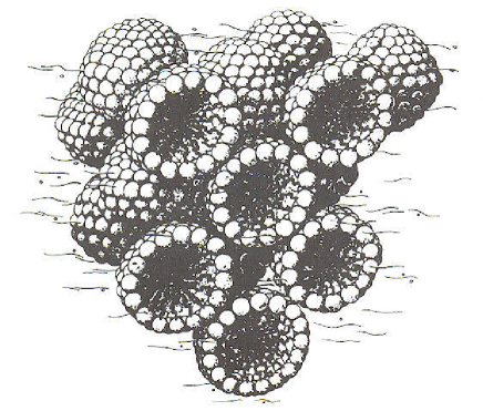
Figure 8: Scheme of micellar structure. The spheres indicate the head groups and the wiggly lines the lipid chains of phospholipids. From C. L. Khetrapal, et al., Lyotropic liquid crystals (Berlin: Springer, 1975).

If we add paraffine oil, close in composition to the hydrocarbon tails of phospholipids, we may stabilize some new phases. A schematic picture of the resulting phase diagram is found in ref. [32] (fig. 10).

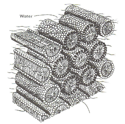
Figure 9: Scheme of hexagonal close-packed structure. From C. L. Khetrapal, et al., Lyotropic liquid crystals (Berlin: Springer, 1975).

The new phenomena are determined by the fact that, if the oil content is large enough, amphiphilic molecules can form a monolayer, with their tails towards the oil-rich phase and their heads towards the water-rich one.

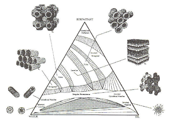
Figure 10: Schematic oil-water-surfactant phase diagram with microstructures depicted. From H. T. Davis et al., in J. Meunier, D. Langevin, N. Boccara (eds.), Physics of amphiphilic layers (Berlin: Springer, 1987) p. 311.

This opens the way to bicountinuous phases, in which both the oil-rich and the water-rich phases percolate. Some of these phases have a periodic, cubic structure, similar to that represented by the cartoon in fig. 10: the actual structures are however more complex and difficult to draw. They are collectively known as ”plumber’s nightmare” phases, since they may be considered as pipeworks in which the interior and the exterior look the same. Of great interest, both theoretical and experimental, are the irregular bicontinuous phases. As shown from the phase diagram, they can be obtained by adding oil to a water-amphiphile solution (with a high enough amphiphile content), without crossing any phase barrier. Moreover they can coexist with the water-rich and the oil-rich phases, having a water-oil ratio close to one. In this coexistence they will remain between the water and oil phases because of their density, and are known therefore as middle-phase microemulsions. The name microemulsions intimates that they are formed of almost equal proportions of oil and water, like ordinary emulsions: however, whereas emulsions are nonequilibrium structures obtained by suspending droplets, say, of oil in water by means of intense mixing, microemulsions are equilibrium phases. In nonequilibrium emulsions, the droplet size ranges from the micrometer to a fraction of millimeter, whereas in microemulsions one observes irregularities in the local composition at scales of the order of a few hundred Ångströms, much smaller than the wavelength of visible light. As a consequence, microemulsions usually appear transparent.

There is also the rather paradoxical possibility that the bilayer forms an interface separating two percolating domains occupied by the same solvent. This is known as the sponge phase [105].

The structure of these phases can be studied by the “traditional” means of light or X-ray diffraction (depending on the characteristic size of the structures), but can be also directly exhibited by freeze fracture. In this technique the sample is rapidly frozen to the temperature of liquid nitrogen. The frozen sample is then fractured by means of a microtome knife. Cleavage usually occurs in the middle of bilayers. The exposed regions can then be shadowed with carbon or platinum, which produces a replica of the interior of the bilayer. In order to expose the exterior of the membrane, one can combine freeze fracture with etching. First, the interior of a frozen membrane is exposed by fracturing; then, the ice that covers one of the adjacent membrane surfaces is sublimed away: this process is called deep-etching. The combined technique, called freeze-etching electron microscopy, provides a view of the interior of a membrane and of both its surfaces. The structure of emulsion and microemulsions can also be exhibited in this way.

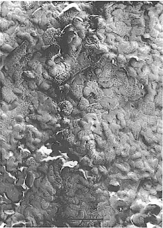
Figure 11: Freeze-fracture of a bicontinuous microemulsion containing equal volumes of water and oil. The shadow material decorates the oil-rich parts of the fracture face. Bar: 500 nm. From W. Jahn, R. Strey, in J. Meunier, D. Langevin, N. Boccara (eds.), Physics of amphiphilic layers, (Berlin: Springer, 1987) p. 354.

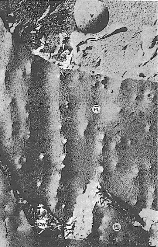
Figure 12: Freeze-fracture of a cell membrane from an onion root tip. The uppermost area in the photograph is the cell cytoplasm with a vacuole (V) evident. The center area shows the fracture face of the cell membrane (plasmalemma, PL). The fracture has also ruptured the cell wall (CW). Plasmodesmata (P), fine threads connecting the cytoplasm of adjacent cells, have also been broken off. From D. Branton, D. W. Deamer, Membrane structure (Berlin: Springer, 1972).

By use of these techniques it has been possible to prove the general validity of the fluid mosaic model of cell membranes, proposed by S. J. Singer and G. Nicholson in 1972 [111]. It may be schematically represented by the cartoon in fig. 12. The main part of the membrane is formed by a bilayer, which is a mixture of several kinds of amphiphilic molecules, in particular phospholipids and glycolipids (sugar-containing lipids, like in particular sphingomyeline and cerebroside), plus smaller ones like cholesterol. Integral membrane proteins are dissolved in the bilayer: they can freely diffuse laterally, but cannot move out of the surface. Other proteins carry hydrophilic tails (sometimes containing sugar: one then speaks of glycoproteins) which extend in the exterior of the cell. In the interior of the cell there is often a network of filaments, suitably anchored to the bilayer. This is the case in particular of the red blood cells (erythrocytes), whose skeleton is formed by filaments of spectrin bound to “buoys” formed by other proteins, like ankyrin and “protein 4.1”.

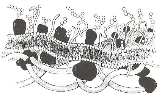
Figure 13: Schematic illustration of a biological membrane (courtesy of Ove Broo Sørensen of the Danish Technical University). The membrane itself is a mixture of several kinds of phospholipids, plus smaller amphihilic molecules, among which (in animals) cholesterol has a prominent role. The dark objects traversing the membranes are “integral membrane proteins”. Other, more flexible, membrane proteins carry carbohydrates (represented as small polygons) in their exterior. The rubber-like cytoskeleton attached to the inner side of the membrane exerts a strong influence on the mechanical properties of the composite membrane.

The fluidity of biological membranes can be exhibited by fluorescence photobleaching recovery experiments in intact cells. One first attaches a fluorescent dye to a specific membrane component. One then looks at a small region ($\sim 3\mu{\rm m}^{2}$) through a fluorescence microscope. One then destroys the fluorescent molecules in this region with a very intense light pulse from a laser. The fluorescence of this region is then monitored as a function of time. The rate of recovery is related to the diffusion coefficient $D$ of the fluorescent-labeled molecules. The order of magnitude of $D$ turns out to be $10^{-8}\,{\rm cm}^{2}{\rm s}^{-1}$, implying that a molecule can diffuse about $2\mu{\rm m}$ in $1\,{\rm s}$. On the other hand, the characteristic times for a molecule to pass from one membrane layer to the other (flip-flop) are of the order of several hours. These times can be measured, although with some difficulty, by NMR [74]. Therefore any asymmetry of the lipid bilayer can be preserved for long periods.

Of course a biological membrane is extremely complex to characterize physically. A strong tendency has therefore developed towards the study of model membranes, containing just one (or two) phospholipids, and in case a controlled concentration of impurities. For example, one can suspend the amphiphile in an aqueous medium, and the agitate the mixture by high-frequency sound waves. This procedure is called sonication. Alternatively, on can dissolve the lipid in ethanol, and then inject the solution via a fine needle into water. In this way one obtains aqueous compartments closed by a lipid bi- or (more often) multi-layer. These structures are called lipid vesicles or liposomes. It is of course possible to prepare the liposomes in a solution containing some interesting drug, and then separate them from the surrounding solution by dialysis or by gel filtration. This technique provides in principle a way to control the delivery of drugs to target cells.

3 Isolated membranes: the Helfrich hamiltonian

In this section I shall discuss the fundamentals of the physical description of isolated membranes: I shall neglect therefore the interaction between membranes, and I shall not consider the microscopic mechanism leading to their formation.

We can write the free energy of a bilayer composed of $2N$ amphiphilic molecules immersed in water as a function of the area $a=A/N$ per molecule [10]:

$$F=2N\phi(a)=2N\left[\phi_{\rm phob}(a)+\phi_{\rm phil}(a)+\phi_{\rm int}(a)\right].$$ (3.1)

In this equation, $\phi(a)$ is the chemical potential of molecules in the bilayer, $\phi_{\rm phob}$ and $\phi_{\rm phil}$ are the effective attractive and repulsive parts, respectively, due to their interaction with water, while $\phi_{\rm int}$ is a direct interaction between amphiphiles which will generically be repulsive. In general, $\phi(a)$ will have a minimum at some preferred area-per-molecule $a=a_{0}$. If the membrane does not exchange molecules with the reservoir, and if it can freely adjust its total area, the equilibrium will be reached when

$$\left.\frac{\partial F}{\partial a}\right|_{a_{\rm eq}}=0,$$ (3.2)

implying

$$a_{\rm eq}=a_{0}.$$ (3.3)

Therefore, the surface tension $\gamma(a)$ of the membrane vanishes at equilibrium:

$$\gamma\left(a_{\rm eq}\right)=\left.\frac{\partial F}{\partial A}\right|_{a_{\rm eq}}=\left.\frac{\partial\phi}{\partial a}\right|_{a_{0}}=0.$$ (3.4)

This simple thermodynamic argument is usually evoked to explain why the surface tension of amphiphilic membranes can be very small.

If we consider a fluctuating amphiphilic membrane, it is necessary to distinguish between its total area $A$ and its projected area $A_{\rm p}$ [31]. To fix one’s ideas, suppose that the membrane spans a planar frame of area $A_{\rm p}.$ If the compressibility of the amphiphilic monolayers is low, the total area $A$ is proportional to the total number $2N$ of molecules forming the membrane: $A=a_{0}N.$ It can only vary through changes in the number of molecules $N.$ Then the two quantities $A$ and $A_{\rm p}$ can be considered as independent thermodynamic variables [10]. They are both extensive: their thermodynamic conjugates represent distinct physical quantities. The area coefficient conjugate to the total area $A,$ which we denote by $\gamma,$ is for incompressible fluids directly proportional to the chemical potential $\mu$ of amphiphilic molecules. The film tension conjugate to the projected area $A_{\rm p},$ which we denote by $\tau,$ corresponds to the physical “surface tension”. One can then consider four different thermodynamical ensembles:

1. $(A,A_{\rm p})$-ensemble: isolated, framed membranes.

2. $(A,\tau)$-ensemble: isolated, unframed membranes.

3. $(\gamma,A_{\rm p})$-ensemble: open, framed membranes.

4. $(\gamma,\tau)$-ensemble: open, unframed membranes.

Experimentally, the most important situations are the open, framed systems (which can be experimentally realized in black lipid films or monolayers) and the isolated, unframed systems, in which the projected area can fluctuate, which correspond to the case of lipid vesicles (at least as long as exchange of lipids with the surrounding solution can be neglected).

Open, framed systems.

In this ensemble the projected area $A_{\rm p}$ is fixed and the total area $A$ fluctuates. The fluctuations are governed by a hamiltonian of the form

$${\cal H}=\gamma A+{\cal H}_{\rm el},$$ (3.5)

where ${\cal H}_{\rm el}$ contains the contribution of elastic internal forces (bending energy, shear modulus, etc.). The partition function is written as the sum over all film configurations ${\cal C}$ with fixed $A_{\rm p}$:

$$Z_{O}=\sum_{\cal C}\exp\left\{-\frac{{\cal H}({\cal C})}{k_{\rm B}T}\right\}.$$ (3.6)

The free energy in this ensemble is

$$G_{O}(\gamma,A_{\rm p})=-k_{\rm B}T\ln Z_{O}(\gamma,A_{\rm p}),$$ (3.7)

and the film tension is simply defined as the free energy per unit projected area:

$$\tau=\lim_{A_{\rm p}\to\infty}\frac{G_{O}(\gamma,A_{\rm p})}{A_{\rm p}}.$$ (3.8)

Isolated, unframed systems

In this ensemble the total area $A$ is fixed while the projected area may fluctuate. The thermodynamic potential is obtained from $G_{O}$ by first going to the isolated, framed $(A,A_{\rm p})$ ensemble where both $A$ and $A_{\rm p}$ are fixed, and the thermodynamic potential is obtained by a Legendre transform

$$F_{I}(A_{\rm p},A)=G_{O}(A_{\rm p},r)-\gamma A,\qquad A=\left.\frac{\partial G_{O}}{\partial\gamma}\right|_{A_{\rm p}}.$$ (3.9)

Then one goes to the isolated, unframed film ensemble by a second Legendre transform which defines the associated thermodynamic potential

$$G_{I}(\tau,A)=F_{I}(A_{\rm p},A)-\tau A_{\rm p},$$ (3.10)

where the surface tension $\tau$ is defined by

$$\tau=\left.\frac{\partial F_{I}}{\partial A_{\rm p}}\right|_{A}=\left.\frac{\partial G_{O}}{\partial A_{\rm p}}\right|_{r}.$$ (3.11)

It is clear that in the thermodynamic limit, $A\to\infty,$ the surface tension defined in this ensemble by eq. (3.11) coincides with the surface tension defined for the open, framed system by eq. (3.9).

We can now analyse the meaning of the tension $\tau$ for isolated, unframed systems with fixed total area $A.$ Let us assume that the projected area fluctuates around its mean value $\left<A_{\rm p}\right>.$ This mean value can be obtained by minimizing $F_{I}(A_{\rm p},A)$ with respect to $A_{\rm p},$ while $A$ is fixed. In the thermodynamic limit it is useful to consider the free energy density

$$f=\frac{F_{I}}{A},$$ (3.12)

as a function of the area ratio

$$a_{\rm p}=\frac{A_{\rm p}}{A}.$$ (3.13)

Two situations are then possible, as depicted in fig. 14.

• $f(a_{\rm p})$ has its minimum for a nonzero ratio $0<a_{\rm p}<1$ (fig. 14(a)). The membrane is then said to be flat, since, although shrunk due to thermal fluctuations, it still keeps the global structure of a two-dimensional object. In this case, eq. (3.11) implies that the surface tension vanishes.

• $f(a_{\rm p})$ has its minimum at $a_{\rm p}=0$ (fig. 14(b)). The membrane is then said to be crumpled, since it is so shrunk by thermal fluctuations that its extension in space does not scale linearly with its internal tension. In this case it is obvious from fig. 14(b) that the tension $\tau$ has in general no reason to vanish: however, there might be marginal situations in which, although the minimum of $f(a_{\rm p})$ is at $a_{\rm p}=0,$ its slope at this point vanishes, and one has therefore $\tau=0.$

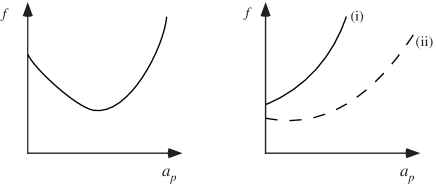
Figure 14: The free energy density $f$ as a function of the area ratio $a_{\rm p}$. (a) $f$ has a minimum for $a_{\rm p}>0$ and the tension $\tau$ vanishes. (b) $f$ has its minimum at $a_{\rm p}=0$ and the tension $\tau$ may either be positive (i) or zero (ii).

Let us consider a fluid membrane freely fluctuating in a solvent. We assume that its thickness is much smaller than the length scales describing its shape and its undulations. Its fluidity implies that all the internal degrees of freedom, related, e.g., to the hydrocarbon chain conformation, the local molecular density, etc., reach equilibrium on a fast time scale. We are thus led to the conclusion that the free energy of the membrane depends on its shape alone. In our hypotheses, we may describe its shape as a geometrical surface.

The curvature of a surface can be described by two quantities, the mean curvature $H$, and the Gaussian curvature $K$. Consider a portion of the surface around an arbitrary point O, like the one depicted in fig. 15. Draw the tangent plane through O and choose the local coordinate axes $(t^{1},t^{2},t^{3})$ so that O is their common origin, $t^{1}$ and $t^{2}$ lie on the plane, and $t^{3}=h$ is normal to it. The surface is locally represented by a quadratic form:

$$h=\frac{1}{2}\sum_{i,j=1}^{2}\Omega_{ij}t^{i}t^{j}+\ldots$$ (3.14)

The matrix $\Omega=\left(\Omega_{ij}\right)$ obviously vanishes for a locally flat surface. This expression of the distance $h$ from the tangent plane in terms of Cartesian coordinates on it, is also called the second fundamental form of the surface. The curvature is defined via the invariants of the second fundamental form, namely:

• The mean curvature $H$ is given by $H={\rm Tr}\,\Omega;$

• The Gaussian curvature $K$ is given by $K={\rm Det}\,\Omega.$

The eigenvalues $c_{1}$, $c_{2}$ of $\Omega$ are called the principal curvatures. They are the inverse of the curvature radii of the intersections of the surface with two planes containing the normal to the surface, and mutually perpendicular. The intersections of these planes with the tangent plane define the principal curvature directions. The principal curvatures are the extreme values of the curvature of any intersection of the surface with a normal plane. In the exceptional case where $c_{1}=c_{2}$, the point O is called an umbilical point, and the principal directions are not defined. The mean curvature $H=c_{1}+c_{2}$ is positive (negative) if the surface is locally mostly above (below) the tangent plane, going in the positive direction along the normal. The Gaussian curvature $K=c_{1}c_{2}$ is positive if the surface is locally on one side of the tangent plane (elliptic point), and negative if it is on both sides (hyperbolic point).

Figure 15: The tangent plane at a point O. The distance of a generic point P from it is given by $h={{1}\over{2}}\sum_{ij}\Omega_{ij}t^{i}t^{j}$. The principal directions on the surface at the point O are also drawn.

The curvatures $H$ and $K$ have a simple geometrical interpretation. Consider a small portion $S$ of the surface, and let $\Delta A$ be its area. Construct now a new surface $S^{\prime}$ by displacing each point of $S$ of a distance $\delta$ along the normal, in the direction of positive $h$. The new surface will have the area

$$\Delta A^{\prime}=\Delta A\,\left(1+\delta H+\delta^{2}K+o(\delta^{2})\right).$$ (3.15)

We now make the following assumptions on the free energy of membranes:

• The surface is smooth, and can be locally represented by the parametric equation $\vec{r}=\vec{r}(\underline{\sigma})$, where $\vec{r}$ denotes a point in three-dimensional ambient space, and $\underline{\sigma}=(\sigma^{1},\sigma^{2})$ are local coordinates of the surface. The function $\vec{r}(\underline{\sigma})$ is differentiable an arbitrary number of times.

• The free energy can be expressed as a local functional of $\vec{r}(\underline{\sigma})$ and its derivatives. This assumption rules out, for the time being, the effects of the interaction of the membrane with itself, due for example to close contacts when a part of the membrane folds on the rest.

• The free energy must be invariant under Euclidean transformations applied to $\vec{r}$ and under reparametrization transformations like $\underline{\sigma}\to\underline{\sigma}^{\prime}=\underline{\sigma}^{\prime}(\underline{\sigma})$.

It was noticed by Canham [14] and then by Helfrich [55] that these hypotheses imply that, considering only the contributions of derivatives of $\vec{r}$ up to second order, one obtains the following general expression of the free energy of a membrane:

$$F=\int_{S}{\rm d}A\,\left[\gamma+\frac{1}{2}\kappa\left(H-H_{0}\right)^{2}+\overline{\kappa}K\right].$$ (3.16)

Here ${\rm d}A$ is the area element and $\gamma$ is the area coefficient. The integral is extended over the membrane surface $S$. The coefficients $\kappa$ and $\overline{\kappa}$ are known as the rigidity and Gaussian rigidity respectively. The quantity $H_{0}$ is called the spontaneous curvature.

The free energy (3.16) has been derived only on the basis of geometrical considerations. However it is necessary to gain some insight on the terms appearing in this expression by considering in more detail the elasticity of a fluid membrane. One finds several discussions of this subject in the literature [99, 116, 57],[86, App. B].

The simplest derivation starts by considering a monolayer. Let us assume that the elastic energy per molecule in a given configuration is the sum of the energy ${\cal E}_{\rm h}$ pertaining to the heads and the energy ${\cal E}_{\rm t}$ pertaining to the tails. We take as a reference the neutral surface, where the moments of the elastic forces on heads and tails cancel. We assume for definiteness that the positive direction is towards the heads, and denote by $\delta_{\rm h}$ and $\delta_{\rm t}$ the distance of the heads and the tails, respectively, from the reference surface.

The areas $a_{\rm h}$ of the heads and $a_{\rm t}$ of the tails are given by:

$$a_{\rm h} = a\left(1+H\delta_{\rm h}+K\delta_{\rm h}^{2}+\ldots\right),$$ (3.17)

$$a_{\rm t} = a\left(1-H\delta_{\rm t}+K\delta_{\rm t}^{2}+\ldots\right),$$ (3.18)

where $a$ is the area of the molecule on the neutral surface (cf. fig. 16).

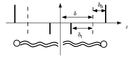
Figure 16: Simple model of a bilayer in an aqueous medium. One assumes that the stresses are localized on the heads and tails of the amphiphilic molecules. The position of the neutral surfaces is denoted by the broken lines.

We can now write, assuming a simple (Hooke-like) elasticity:

$${\cal E}_{\rm h} = \frac{1}{2}k_{\rm h}\left(\frac{a_{\rm h}-a_{{\rm h}0}}{a_{{\rm h}0}}\right)^{2},$$ (3.19)

$${\cal E}_{\rm t} = \frac{1}{2}k_{\rm t}\left(\frac{a_{\rm t}-a_{{\rm t}0}}{a_{{\rm t}0}}\right)^{2},$$ (3.20)

where $a_{{\rm h}0}$ and $a_{{\rm t}0}$ are the equilibrium values of head and tail areas, and $k_{\rm h}$ and $k_{\rm t}$ are elastic constants (with the dimensions of an energy per molecule). The elastic energy ${\cal E}$ per unit molecule can be written

$${\cal E}={\cal E}_{\rm h}+{\cal E}_{\rm t}.$$ (3.21)

For a flat membrane we can obtain from it the expression of the elastic energy of compression per unit area:

$${\cal H}^{({\rm m})}_{\rm comp}=\frac{{\cal E}}{a_{0}}=\frac{E_{0}}{a_{0}}+\frac{1}{2}k^{({\rm m})}\left(\frac{a-a_{0}}{a_{0}}\right)^{2},$$ (3.22)

where $E_{0}$ is a constant, and where the compression modulus $k^{({\rm m})}$ and the equilibrium area per molecule $a_{0}$ are respectively given by

$$k^{({\rm m})} = \frac{k_{\rm h}}{a_{{\rm h}0}}+\frac{k_{\rm t}}{a_{{\rm t}0}},$$ (3.23)

$$a_{0} = k^{({\rm m})}\bigg{/}\left(\frac{k_{\rm h}}{a_{{\rm h}0}^{2}}+\frac{k_{\rm t}}{a_{{\rm t}0}^{2}}\right)=\frac{k^{({\rm m})}}{\beta_{\rm h}+\beta_{\rm t}}.$$ (3.24)

The index $({\rm m})$ reminds us that we are dealing with a monolayer. The condition that the moments of the compression forces vanish on the neutral surface implies $\delta_{\rm h}\beta_{\rm h}=\delta_{\rm t}\beta_{\rm t}.$ We can now let the expression of the areas $a_{\rm t}$ and $a_{\rm h}$ in the expression of the elastic energy, obtaining

$${\cal F}^{({\rm m})} = {\cal H}^{({\rm m})}_{\rm comp}+{\cal H}^{({\rm m})}_{\rm bend}=$$ (3.25)

$$=\sigma^{({\rm m})}+\frac{1}{2}k^{({\rm m})}\left(\frac{a-a_{0}}{a_{0}}\right)^{2}+\frac{1}{2}\kappa^{({\rm m})}\left(H-H_{0}^{({\rm m})}\right)^{2}+\overline{\kappa}^{({\rm m})}K,$$

where

$$\sigma^{({\rm m})} = \frac{E_{0}}{a_{0}},$$ (3.26)

$$\kappa^{({\rm m})} = (\delta_{\rm h}+\delta_{\rm t})^{2}k^{({\rm m})}\frac{\beta_{\rm h}\beta_{\rm t}}{(\beta_{\rm h}+\beta_{\rm t})^{2}}=\delta_{\rm h}\delta_{\rm t}\,k^{({\rm m})},$$ (3.27)

$$\overline{\kappa}^{({\rm m})} = (a_{{\rm h}0}-a_{{\rm t}0})\frac{\beta_{\rm h}\beta_{\rm t}(\beta_{\rm h}-\beta_{\rm t})}{(\beta_{\rm h}+\beta_{\rm t})^{2}},$$ (3.28)

$$H_{0}^{({\rm m})} = \frac{\overline{\kappa}}{\kappa}\frac{1}{\delta_{\rm h}-\delta_{\rm t}}.$$ (3.29)

We see that $\kappa^{({\rm m})}>0,$ while $\overline{\kappa}^{({\rm m})}$ can be of either sign. We can now estimate the order of magnitude of the rigidities $\kappa^{({\rm m})}$, $\overline{\kappa}^{({\rm m})}$. For pure phospholipids the measured compressibility is $k\sim 50\,{\rm dyn}/{\rm cm}=5\,10^{-1}\,{\rm Jm}^{-1},$ and the distances $\delta_{\rm h},$ $\delta_{\rm t}$ are of the order of $10\,{\rm\AA}.$ We obtain therefore $\kappa^{({\rm m})}\sim 5\,10^{-20}{\rm J},$ which must be compared with the termal energy $k_{\rm B}T\sim 4.2\,10^{-21}J$ at $T=300\,{\rm K}.$ The fact that typical rigidities are only slightly larger than the thermal energy makes fluctuations important in understanding the behavior of amphiphilic membranes.

We can now consider a bilayer, by putting two monolayers, called “internal” (i) and “external” (e) on the top of each other. We assume that there are no interactions between the monolayers, so that

$${\cal F}_{\rm b}={\cal F}^{({\rm m})}_{{\rm i}}+{\cal F}^{({\rm m})}_{{\rm e}},$$ (3.30)

where the suffixes refer to the two monolayers. We denote by $a_{i}$ the area per molecule of the monolayer $i={\rm i},\,{\rm e},$ measured on its neutral surface. We can thus define the particle density $\rho_{i}$ of each monolayer, measured along a bilayer reference surface, placed midway between the two neutral surfaces of the monolayers. Let us denote by $\delta$ the distance between the bilayer reference surface and that of the monolayers. For a bilayer with heads outside, for example, we have $\delta=\delta_{\rm t}.$ We choose the positive direction on the normal, in going, e.g., from the internal to the external layer. We then have

$$\frac{1}{\rho_{{\rm i}}} = a_{{\rm i}}\,(1-H\delta+K\delta^{2}+\ldots),$$ (3.31)

$$\frac{1}{\rho_{{\rm e}}} = a_{{\rm e}}\,(1+H\delta+K\delta^{2}+\ldots).$$ (3.32)

This allows us to define the mean density $\overline{\rho}$ and the density difference $\tilde{\rho}$:

$$\overline{\rho} = \frac{\rho_{{\rm i}}+\rho_{{\rm e}}}{2},$$ (3.33)

$$\tilde{\rho} = \frac{\rho_{{\rm i}}-\rho_{{\rm e}}}{2}.$$ (3.34)

In the case where the spontaneous curvature $H_{0}$ of each monolayer vanishes, one obtains the following expression of the elastic energy density per unit area of the bilayer:

$${\cal F}_{\rm b} = \sigma_{\rm b}\overline{\rho}a_{0}+\frac{1}{2}k_{\rm b}\left(a_{0}\overline{\rho}-1\right)^{2}+\frac{1}{2}k_{\rm b}(a_{0}\tilde{\rho})^{2}$$ (3.35)

$$+a_{0}k_{\rm b}D\tilde{\rho}H+\left(2\kappa_{\rm b}+\frac{k_{\rm b}\delta^{2}}{2}\right)H^{2}+\overline{\kappa}_{\rm b}K.$$

In this equation, the bilayer parameters (denoted by the suffix (b)) are simply the sum of the corresponding parameters of the monolayers.

If the spontaneous curvature of the monolayers does not vanish, but the two monolayers are made of the same material, one obtains the same expression, but with slightly renormalized values of the elastic parameters. In either case, the spontaneous curvature $H_{0}$ of the bilayer vanishes.

The only difference with respect to the Helfrich hamiltonian lies in the terms depending on the particle densities $\overline{\rho},$ $\tilde{\rho},$ which we now discuss. The first term, $\sigma_{\rm b}\overline{\rho}a_{0},$ yields a contribution proportional to the total number $2N$ of molecules in the membrane, but independent of its geometry. It corresponds to a shift in the chemical potential of the amphiphile. As long as one considers vesicles over short time scales, so that amphiphilic molecules are not exchanged with the solvent, this term plays no role. The second term represents the energy cost necessary to induce local density fluctuations. As we have seen, the rigidity $\kappa_{\rm b}$ is of the order of $k_{\rm b}\delta_{\rm h}\delta_{\rm t}$: therefore, it costs about the same energy to bend the membrane with a radius of the order $10^{3}\delta\sim 1\,\mu{\rm m}$ as to produce a change of order $10^{-3}$ in the relative area $(A-A_{0})/A_{0},$ where $A_{0}=Na_{0}.$ From a practical point of view, therefore, the membrane can be considered incompressible and its area can be set equal to $A_{0}.$ The third term represents a coupling between the local density difference between the two monolayers and the mean curvature $H.$ Indeed, if we try to bend the membrane, the molecules contained in the interior layer are compressed with respect to those contained in the exterior layer, and therefore tend to escape.

Let us now consider a closed vesicle, formed by a bilayer with identical monolayers. If the observation times are not too long (of the order of several hours, or even a few days) the total number of molecules contained in the bilayer remains constant: on the other hand, as we have seen, the “flip-flop” times are also quite long, and therefore the number of molecules contained in each monolayer can be considered constant. Therefore the integrals of both $\overline{\rho}$ and $\tilde{\rho}$ over the whole bilayer surface are constant. In particular, that means that their average values are given by

$$\overline{\rho}_{0} = \frac{N_{\rm i}+N_{\rm e}}{2A},$$ (3.36)

$$\tilde{\rho}_{0} = \frac{N_{\rm i}-N_{\rm e}}{2A},$$ (3.37)

where $N_{\rm e,i}$ are the number of molecules in the two monolayers, and $A$ is the area of the vesicle. Therefore the term $\oint{\rm d}A\gamma\overline{\rho}a_{0}$ is independent of the bilayer shape. It is reasonable to assume, in view of the fast lateral diffusion times of the amphiphiles, that $\tilde{\rho}$ locally equilibrates faster than the vesicle shape. It will then assume locally the value dictated by the optimization of $F_{\rm b}$ when the curvatures are kept fixed. One has

$$\tilde{\rho}(\vec{r})=\tilde{\rho}_{0}+\delta\tilde{\rho}(\vec{r}),$$ (3.38)

where $\delta\tilde{\rho}$ satisfies

$$\delta\tilde{\rho}=-\tilde{\rho}_{0}-\frac{\delta}{a_{0}}H.$$ (3.39)

We can use again eq. (3.15) to show that this equation implies

$$\oint_{S}{\rm d}A\delta\tilde{\rho}=0.$$ (3.40)

If we assume that $\overline{\rho}=a_{0}^{-1}$ locally, and let the result for $\delta\tilde{\rho}$ into the expression for ${\cal F}_{\rm b}$ we obtain

$$F_{\rm b}=\oint_{S}{\rm d}A{\cal F}_{\rm b}=\oint_{S}{\rm d}A\left\{\frac{1}{2}\kappa_{\rm b}H^{2}+\overline{\kappa}_{\rm b}K\right\},$$ (3.41)

up to a term independent of the bilayer geometry.

These arguments lead thus to the conclusion that vesicles formed by symmetric bilayers are described by the Helfrich hamiltonian with a vanishing spontaneous curvature. A small asymmetry between the monolayers can be induced by a difference in the solvent: e.g., if a higher concentration in ions screens more effectively on the interior the electrostatic interaction among the heads. One is safe to assume that any induced spontaneous curvature will be rather small. However, the surface must satisfy the additional constraints, fixing the value of (i) the enclosed volume $V$, (ii) the total area $A$, and (iii) the area difference between the two monolayers, which can be expressed in terms of the integral of the mean curvature $H$:

$$\Delta A=2\delta\oint_{S}{\rm d}AH=2\delta M.$$ (3.42)

This model of a vesicle, due to Svetina et al. [115], is known as the bilayer coupling (BC) model. The earlier work on vesicle shapes had considered the spontaneous curvature as an independent parameter, and had neglected the constraint on the integral of the mean curvature. This model has is known as the spontaneous curvature (SC) model. Although the spontaneous curvature $H_{0}$ can be considered as the conjugate variable to the integral of the mean curvature $M$, the two descriptions are not equivalent. The point to keep in mind is that the Helfrich curvature energy does not grow with the size of the system as an extensive free energy, in the way one is accustomed to find in thermodynamical systems. In fact, it is scale invariant: consider a surface $S$ defined by some parametric equation of the form $\vec{r}=\vec{r}_{0}(\overline{\sigma})$. Now define the new surface $S^{\prime}$ by the parametric equation $\vec{r}=\lambda\vec{r}_{0}(\overline{\sigma})$, where $\lambda>0$. In this transformation, we have

$$H \to H^{\prime}=\lambda^{-1}H;$$ (3.43)

$$K \to K^{\prime}=\lambda^{-2}K;$$ (3.44)

$${\rm d}A \to {\rm d}A^{\prime}=\lambda^{2}{\rm d}A.$$ (3.45)

Therefore the elastic energy remains locally invariant: on the other hand, since $H$ (and therefore $M$) is multiplied by $\lambda^{-1}$, the corresponding conjugate field $H_{0}$ should be multiplied by $\lambda$ in order to keep the “scaled” constraint. Since the differential ${\cal F}_{\rm b}{\rm d}A$ of $F_{\rm b}$ remains locally invariant upon a scale transformation, it will be invariant upon all transformations which locally reduce to a scale transformation (plus translations and rotations) [119]. This form the class of conformal transformations, which in three dimensions are obtained as the group formed by translations, rotations and a three-parameter family of special conformal transformations, obtained as the combination of an inversion, a translation, and another inversion. Of course, the constraints mentioned above are not invariant in general upon such a transformation. From now on, we shall only refer to bilayers, and correspondingly drop the (b) suffix on the rigidity moduli.

4 Vesicle shapes

The theory of the equilibrium shapes of phospholipid vesicles started in 1970, when Canham [14] showed that the characteristic discoidal shape of red blood cells (erythrocytes) can be obtained by the minimization of the curvature elastic energy for a particular value of the area and enclosed volume costraints. Actually the case of the red blood cells, although of great interest, is somehow misleading, since the spectrin-ankyrin network present on the interior of the red blood cell membrane makes its properties somehow different from those of a fluid membrane [38, 8].

An extensive study of vesicle shapes was performed by Deuling and Helfrich in the seventies [34, 33]. The problem was reconsidered more recently, in particular because of the experiments of the Sackmann group [4, 70, 71], which exhibited shape transitions of single vesicles induced by changes in temperature. This prompted the research on the identification of the phase diagram of vesicle shapes (for recent reviews, see, e.g., [80], and the Proceedings contained in [82]). The interest has been further enhanced by the observation of toroidal vesicles by Mutz and Bensimon [92], which has stimulated several investigations on vescles with higher genus [107, 108, 87, 86].

In the spirit of mean field theory, the shape of a vesicle is obtained by minimization of the elastic free energy (3.16)

$$F=\oint_{S}{\rm d}A\,\left\{\frac{1}{2}\kappa H^{2}+\overline{\kappa}K\right\}.$$ (4.1)

For phospholipids, $\kappa\sim 10^{-19}$ J [37, 91]. This expression of the energy also yields a nice argument to explain why isolated membranes form vesicles at all. Indeed the elastic free energy $F$ of any given shape is independent of its scale: e.g., for a sphere one has

$$F=8\pi\kappa+4\pi\overline{\kappa}.$$ (4.2)

If the membrane is not closed, but has a free edge of length $\ell$, the free energy of the edge will be proportional to $\ell$, times some line tension $\tau,$ which is of the order of $10^{-20}$–$10^{-19}$ J nm^-1 [53, 43]. As soon as the lateral size of the membrane becomes larger than $\kappa/\tau,$ i.e., 1–10 nm, it becomes energetically favorable for the membrane to get rid of its open edge and form a closed vesicle. A detailed study of this transition, analytic at zero temperature, and via simulations at $T>0,$ is contained in ref. [7].

The bilayer is relatively permeable to water [21], much less to ions: the permeability ratio is of order $10^{9}$. On a time scale of several hours the ions enclosed in the vesicle at its formation remain there. As a consequence, any variation in the enclosed volume—due to the permeation of some amount of water—would lead to the apperance of an osmotic pressure. Equilibrium is reached when the osmotic pressure balances the membrane tension. On the other hand, the time needed to exchange amphiphilic molecules between the two layers, or between the bilayer and the solution, are of the order of several hours. Therefore, as long as we consider shorter times, we can argue that the enclosed volume $V$, the total bilayer area $A$, and the number of molecules contained in each bilayer are constant. The last constraint, as we have seen, is equivalent to a constraint on the total mean curvature $M=\oint{\rm d}A\,H.$ These constraints can be taken into account by Lagrange multipliers, which correspond to the pressure difference $p$ between the interior and the exterior, the lateral tension $\gamma,$ and a quantity $\mu$ proportional to a variation of the spontaneous curvature. In principle, one cannot rule out the possibility that a small spontaneous curvature $H_{0}$ is present. The Euler-Lagrange equations read

$$\delta\left(F+pV+\gamma A+\mu M\right)=0.$$ (4.3)

It is a consequence of the Gauss-Bonnet theorem that the Gaussian curvature term does not play any role in this variational problem. According to this theorem, the integral $\oint{\rm d}A\,K$ is a topological invariant:

$$\oint_{S}{\rm d}AK=4\pi\chi_{\rm E},$$ (4.4)

where $\chi_{\rm E}$ is the Euler-Poincaré characteristic, equal to one minus the number of “handles” of the surface: i.e., it is equal to 1 for the sphere, to 0 for the torus, to -1 for the torus with two holes… The last term in (3.16) remains therefore constant for all continuous deformations of a given surface. The variational equation depends only on the parameters $p$, $\gamma$, $\kappa$ and $H_{0}.$ The solution of the Euler-Lagrange equations will be characterized by the values $V$ of the volume, $A$ of the area, and $M$ of the total mean curvature. If we now perform the scale transformation $\vec{r}\to\lambda\vec{r}$, we have

$$V \to V^{\prime}=\lambda^{3}V;$$ (4.5)

$$A \to A^{\prime}=\lambda^{2}A;$$ (4.6)

$$M \to M^{\prime}=\lambda M.$$ (4.7)

This shape will be a solution of the same Euler-Lagrange equation, corresponding to the same value of $\kappa$, but where

$$p \to p^{\prime}=\lambda^{-3}p;$$ (4.8)

$$\gamma \to \gamma^{\prime}=\lambda^{-2}\gamma;$$ (4.9)

$$\mu \to \mu^{\prime}=\lambda^{-1}\mu.$$ (4.10)

With these substitutions, the free energy remains invariant.

We can use this scale invariance to draw the phase diagram of vesicle shape as a function of dimensionless variables. One naturally introduces the radius $R_{0}$ as the radius of the sphere having the same area $A$:

$$R_{0}=\left(\frac{A}{4\pi}\right)^{\frac{1}{2}}.$$ (4.11)

One can thus define:

• The reduced volume:

  $$v=\frac{V}{\frac{4}{3}\pi R_{0}^{3}}=6\sqrt{\pi}\frac{V}{A^{\frac{3}{2}}};$$ (4.12)

• The reduced total curvature $m$:

  $$m=\frac{M}{R_{0}}.$$ (4.13)

The resulting Euler-Lagrange equations cannot be analytically solved in general. If one looks for axisymmetric shapes one can transform these equations into a system of first-order ordinary differential equations, which can be solved numerically [34, 96]. In this way one obtains the phase diagrams shown in fig. 17, as a function of $v$ and $\Delta a=m/4\pi$.

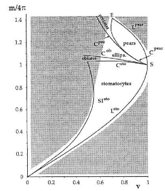
Figure 17: Phase diagram of shapes in the BC model. From K. Berndl, J. Käs, R. Lipowsky, E. Sackmann, U. Seifert, in L. Peliti (ed.) Biologically Inspired Physics (New York: Plenum, 1991).

The continuous lines $C^{\rm pear}$ and $C^{\rm sto}$ denote lines of continuous transitions at which the up/down symmetry of the vesicle shape is broken. $L^{\rm pear}$, $L^{\rm sto}$ and $L^{\rm dumb}$ denote limit shapes. The dumbbell region contains for large $v$-values prolate ellipsoids, and the discocyte region oblate ellipsoids.

The figure also contains pointed lines, labelled by numbers, which correspond to trajectories observed in actual phospholipid vesicles. The photographs of these vesicles are shown in fig. 18, together with the calculated shapes.

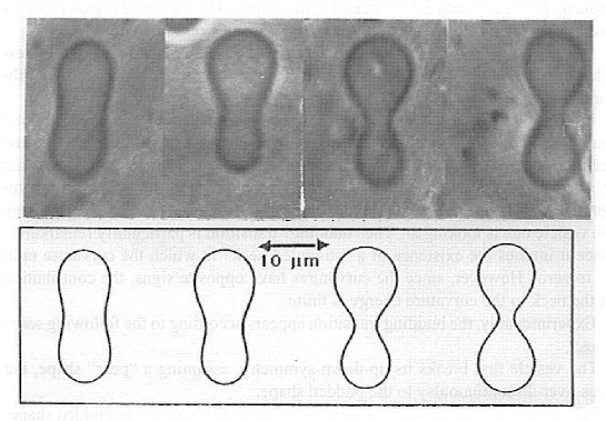
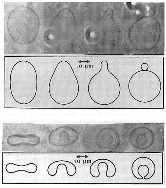
Figure 18: Demonstration (1) of a budding transition; (2) symmetric-asymmetric reentrant transition; (3) discocyte-stomatocyte transition. Vesicles of DMPC in water: the reconstructed trajectories in $(v,m)$ space correspond to the dotted lines in the previous figure. From K. Berndl, J. Käs, R. Lipowsky, E. Sackmann, U. Seifert, in L. Peliti (ed.) Biologically Inspired Physics (New York: Plenum, 1991).

In the interpretation of these experiments, the value of the reduced total curvature $m$ is inferred by the observed shape changes instead of being measured. In order to explain the transitions observed in a given vesicles, one has to assume that the inner and outer layer expand at different rates when the temperature is raised, introducing a phenomenological parameter which depends on the vesicle one is looking at. The “budding” transition is particularly remarkable, since it implies the existence of a “strangled neck” in which the curvature radii go to zero. However, since the curvatures have opposite signs, the contribution of the neck to the curvature energy is finite.

Experimentally, the budding transition appears according to the following scenarios:

• The vesicle first breaks its up-down symmetry, assuming a “pear” shape, the goes over discontinuously to the budded shape;

• The vesicle goes over continuously via a dumbbell shape to the budded shape.

While the second possibility agrees with the calculated phase diagram of the BC model, the first one has some difficulties: the BC model predicts a continuous budding transition, on the other hand the SC model does not predict the intermediate “pear” shape. A model based on area-difference elasticity has been introduced to resolve this difficulty [85]. It seems to me that the continuous elastic model of the membrane breaks down near the strangled neck, which may have an additional energy cost due to the strain it imposes on the phospholipid tails: the extra cost could turn a continuous transition into a discontinuous one.

Mutz et al. first observed toroidal vesicles in partially polymerized vesicles [92]. Vesicles of the same or higher genus have then been observed in fluid vesicles made with the same phospholipid. This observation has aroused great interest, because it opened the possibility of investigating “experimentally” a classic mathematical problem posed by Willmore [119]. He had asked in fact which shapes minimized, for each topological genus, the Willmore functional $W=\oint_{S}{\rm d}AH^{2},$ which is none other than the Helfrich Hamiltonian with zero spontaneous curvature. For genus 0 the solution is shown to be the sphere, and for genus 1 Willmore proposed the conjecture that the solution was the Clifford torus, i.e., the circular torus in which the ratio of the inner circle radius to the outer one is equal to $1/\sqrt{2}.$

However, all images of the Clifford torus upon conformal transformation correspond to the same value of $W.$ There is a family of these images—similar to tori with a non-central hole—known as Dupin cyclids. Therefore, the consideration of conformal invariance paves the way to the study of non axisymmetric shapes. Upon conformal transformations, the reduced volume $v$ and total curvature $m$ are not invariant. In particular, the reduced volume of the Dupin cyclids is always larger that the volume of the Clifford torus, which is equal to 0.71. The minimization of the curvature energy finds therefore its solution (if Willmore’s conjecture is true) if we consider the SC model (without the constraint on the total curvature) and look for surfaces with reduced volume larger that 0.71. Other forms can be obtained by the solution of the differential equations, as it had been done for vesicles of genus 0. One can check the stability of the axisymmetric forms with respect to an infinitesimal conformal transformation which breaks the symmetry. One can thus derive the phase diagram shown in fig. 19 [69].

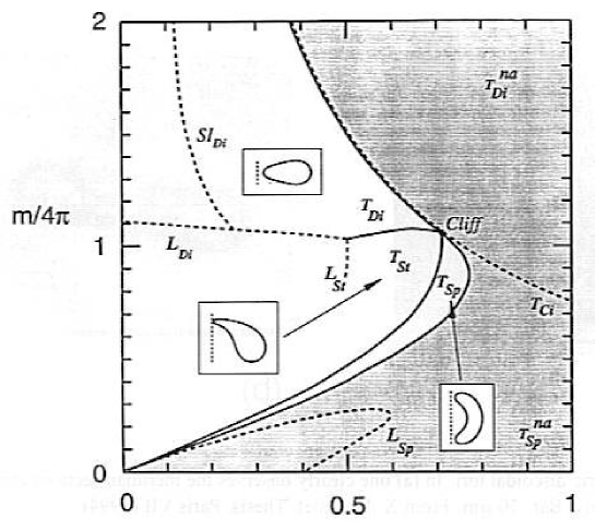
Figure 19: Phase diagram for vesicles of genus 1 in the BC model. Gray areas correspond to non axisymmetric shapes. From F. Jülicher, U. Seifert, R. Lipowsky, J. Phys. II France 3 1681 (1993).

One finds:

• A region of nonaxisymmetric tori ($T^{\rm na}$);

• A region of discoidal tori ($T_{\rm Di}$);

• A region of stomatoidal tori ($T_{\rm St}$);

• A region of spheroidal tori ($T_{\rm Sp}$).

The last three zones have boundaries on the limit curves: $SI_{\rm Di}$, where discoidal tori auto-intersect, and $L_{\rm Di},$ $L_{\rm St},$ $L_{\rm Sp}$ where the diameter of axisymmetric tori vanishes. On the continuous lines which separate $T_{\rm Di}$ from $T_{\rm St}$ and this from $T_{\rm Sp}$ the shapes cross over continuously from one family to the other. All four families have the Clifford torus Cliff in common. Circular tori form the boundary between axisymmetric and non axisymmetric shapes for $m>m_{\rm Cliff}=4\pi\times 2^{-\frac{3}{4}}\pi^{\frac{1}{2}}=4\pi\times 1.05.$ For smaller values of $m,$ this boundary is formed by spheroidal tori. Discoidal tori are equilibrium shapes only within the BC model with zero spontaneous curvature.

Experimentally [86] one finds indeed that vesicles having the Clifford torus shape turn into non axisymmetric shapes (close to Dupin cyclids) upon cooling (which induces a decrease of the bilayer area, and thus an increase in reduced volume) (see fig. 20).

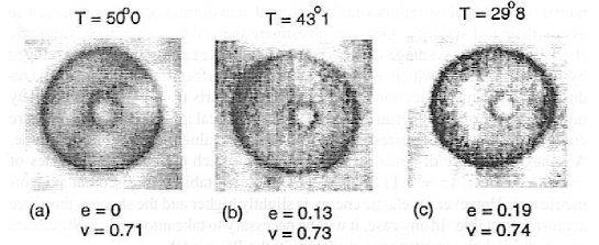
Figure 20: Breaking of axial symmetry of the Clifford torus upon cooling. The transformation is reversible. The parameter $e$ denotes the excentricity of the cyclid. The bar corresponds to 10 $\mu$m. From X. Michalet, Thesis, Paris VII (1994).

One can also observe axisymmetric discoidal tori, supporting the idea that the vesicles are described by the BC model—although one could not rule out the possibility that these shapes are merely metastable (see fig. 21).

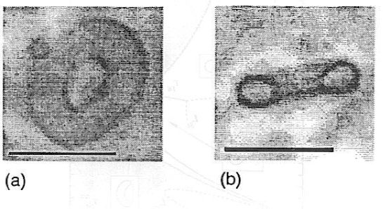
Figure 21: Axisymmetric discoidal tori. In (a) one clearly observes the meridian sections characteristic of the discoidal family. Bar: 10 $\mu$m. From X. Michalet, Thesis, Paris VII (1994).

However, one can also observe nonaxisymmetric discoidal tori, which do not appear as stable shapes in the phase diagram of the BC model with vanishing spontaneous curvature. These shapes cannot be obtained as conformal transforms of a stable axisymmetric shape. This indicates that the stability of axisymmetric shapes against infinitesimal conformal transformations is not enough to assess their full stability. One can investigate the stability of nonaxisymmetric shapes by taking advantage of powerful program Surface Evolver developed by K. A. Brakke [9], which, starting from a given surface shape, lets it evolve reducing the Willmore functional at each step. One starts from a shape obtained by image analysis of the experiment and looks for the local minimum of the curvature energy near to it—and corresponding to the same value of the reduced volume. A nonaxisymmetric discoidal torus is obtained, which corresponds to values of $v=0.52$ and $m/4\pi=1.11,$ well in the region of stability of discoidal axisymmetric tori. However, its elastic energy is slightly higher and the shape is therefore at most metastable. In any case, it will be necessary to take into account the effects of a nonvanishing spontaneous curvature in the BC model.

Vesicles of higher topology have more recently been observed. The important new fact is that for some values of the parameters $v$ and $m$ there is a one-parameter family of conformal transformations which conserves the Willmore functional and satisfies at the same time the constraints [69].

By numerically minimizing a discretized version of the Helfrich hamiltonian, Hsu, Kusner and Sullivan found that the Lawson surface L shown in fig. 22 corresponds to a minimum, with a value $F=F_{2}\simeq 1.742\times 8\pi\kappa$ [64]. This surface has a threefold symmetry axis and an additional mirror symmetry plane: this symmetry is denoted (in the Schönflies notation) by ${\cal D}_{3h}.$ Jülicher, Seifert and Lipowsky [69] developed an algorithm for minimizing the bending energy $F$ for a triangulated surface, and were able to confirm the result of ref. [64]. By applying special conformal transformations to the Lawson surface, one obtains a three-parameter family of surfaces (the Willmore surfaces ${\cal W}$) having the same value $F_{2}$ of the bending energy. By projecting the three-dimensional space ${\cal W}$ onto the two-dimensional space $(v,m),$ where $v$ is the reduced volume and $m$ is the reduced total curvature, one obtains a two-dimensional region $W$ of the plane in which a one-parameter family of special conformal transformations leaves the bending energy invariant by still satisfying the constraints.

Special conformal transformations (SCT) can be parametrized by a vector $\vec{a}=(a_{x},a_{y},a_{z}),$ defined by the transformation rule

$$\vec{r}\to\vec{r}^{\prime}=\frac{\vec{r}/r^{2}+\vec{a}}{\left(\vec{r}/r^{2}+\vec{a}\right)^{2}}.$$ (4.14)

A SCT acting on a surface with initial values $v=v_{1}$ and $m=m_{1}$ generates a new shape with $v=v_{1}(\vec{a})$ and $m=m_{1}(\vec{a}),$ where

$$v_{1}(\vec{a}) = v_{1}\left[1+A^{(v)}_{\alpha}a_{\alpha}+O(\vec{a}^{2})\right],$$ (4.15)

$$m_{1}(\vec{a}) = m_{1}\left[1+A^{(m)}_{\alpha}a_{\alpha}+0(\vec{a}^{2})\right],$$ (4.16)

in which the coefficients $\vec{A}^{(v)}$ and $\vec{A}^{(m)}$ can be expressed as

$$\vec{A}^{(v)} = 6(\vec{R}^{A}-\vec{R}^{V}),$$ (4.17)

$$\vec{A}^{(m)} = 2(\vec{R}^{A}-\vec{R}^{M}),$$ (4.18)

in terms of the center of volume $\vec{R}^{V}=\oint{\rm d}V\vec{R}/V,$ the center of area $\vec{R}^{A}=\oint{\rm d}A\vec{R}/A,$ and the center of mean curvature $\vec{R}^{M}=\oint{\rm d}AH\vec{R}/M.$ Thus, the conformal mode which conserves both $v$ and $m$ can be identified as the SCT with $\vec{a}$ obeying the differential equation

$$\frac{{\rm d}\vec{a}}{{\rm d}s}=\vec{A}^{(v)}\times\vec{A}^{(m)},$$ (4.19)

where $s$ parametrizes the path in the space ${\cal W}.$

The boundaries of the region $W$ can be determined by first introducing the button surface B shown in  22.

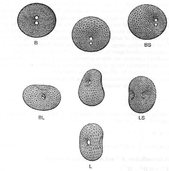
Figure 22: Willmore surfaces with bending energies $F=F_{2}\simeq 1.75\times 8\pi\kappa.$ These shapes correspond to points at the boundary of the region ${\cal W}$: The ${\cal D}_{3h}$ symmetric Lawson surface L; the ${\cal D}_{2h}$ symmetric button surface B; and examples of ${\cal C}_{2v}$ symmetric shapes along the lines $C_{BS},$ $C_{BL},$ and $C_{LS},$ respectively. From F. Jülicher, U. Seifert, R. Lipowsky, Phys. Rev. Lett. 71 452 (1993).

This surface is conformally equivalent to the Lawson surface L and corresponds to $v=0.66,$ and $m=1.084\times 4\pi.$ It has three orthogonal symmetry planes, i.e., symmetry ${\cal D}_{2h}.$ Choose the $(x,y)$ plane to be the midplane of the disk, with the centers of the two holes along the $x$ axis. By applying SCT one can define a line $C_{BL}$ of conformally equivalent surfaces of symmetry ${\cal C}_{2v}$ which connect B to L. This line is defined by $\vec{a}=(0,0,a_{z})$ with $0\leq a_{z}\leq 3.4/R_{0}.$ A further increase in $a_{z}$ breaks the threefold symmetry of L, generating the line $C_{LS}$ with ${\cal C}_{2v}$-symmetric shapes: for $a_{z}=15.5/R_{0},$ the shape along this approaches a sphere with two infinitesimal handles at $(v,m)=(1,4\pi).$ If on the other hand we break the $x$-$z$ symmetry plane of B by a SCT transformation with $\vec{a}=(0,a_{y},0),$ we obtain the line $C_{BS}$ which also approaches a sphere at $(v,m)=(1,4\pi).$ The three lines $C_{BL},$ $C_{LS}$ and $C_{BS}$ form the boundary of the region $W$.

Within this region one should be able to observe fluctuations of the shape of the vesicle among conformal transforms: this phenomenon has been named conformal diffusion and has first been observed by Michalet and collaborators [86]. Examples of this behavior are shown in fig. 23.

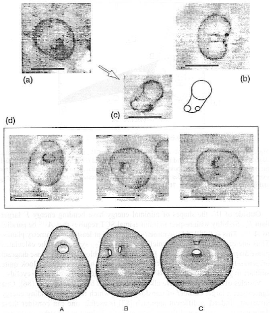
Figure 23: Example of a vesicle of type BS undergoing conformal diffusion. Bar: $10\mu{\rm m}.$ (a): View from “above”, showing the absence of symmetry planes normal to the focal plane. A small rotation leads to view (b) and eventually to view (c). The series of three views (d) shows the vesicle at intervals of a few seconds. From X. Michalet, Thesis, Paris VII (1994).

There is of course the delicate experimental problem of discriminating between conformal diffusion and ordinary thermal fluctuations.

Outside of $W$, the shapes of minimal energy have bending energy $F$ larger than $F_{2}.$ Stability with respect to infinitesimal SCT requires that $\vec{A}^{(v)}$ be parallel to $\vec{A}^{(m)}.$ This is fulfilled by symmetry if there are at least two symmetry planes. Thus one can look for shapes which have at least ${\cal C}_{2v}$ symmetry. The calculated phase diagram is shown in fig. 24.

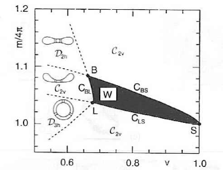
Figure 24: Phase diagram of genus-2 vesicles. Within the region $W$, the ground state is conformally degenerate. This region is bounded by the lines $C_{BS},$ $C_{BL},$ and $C_{LS}.$ The Lawson surface L and the button surface B are special point at the boundary of $W.$ Adjacent to $W,$ five different regions exist. The symmetries of the shapes within these regions are indicated. From F. Jülicher, U. Seifert, R. Lipowsky, Phys. Rev. Lett. 71 452 (1993).

For comparison, a blow up of the phase diagram of genus-1 vesicles is shown in fig. 25.

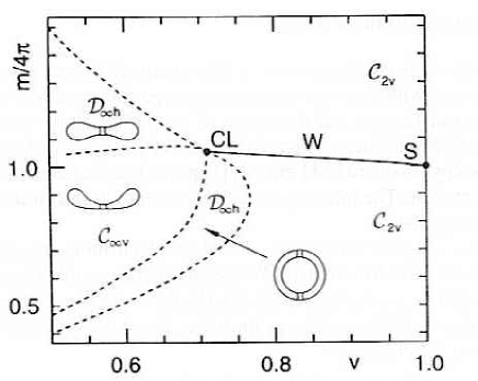
Figure 25: Phase diagram for genus-1 vesicles. The line $W$ denotes the Willmore surfaces (Dupin cyclids) starting at the Clifford torus CL. Compare with the previous figure.

One sees that the diagrams look quite similar: in particular the region $W$ corresponds to the line $W$ of Dupin cyclids.

Vesicles of higher genus have also been observed by Michalet et al. [86]. One can expect a larger number of transformations which leave the bending energy invariant. Indeed, a different approach [87] is useful: one can consider these deformations as positional fluctuations of necks linking two nearby concentric membranes. The strategy is to consider the shape of a neck of radius $a$ linking two square parallel pieces of membrane of size $L\times L$ with periodic boundary conditions. The problem breaks into a inner problem, in which the surface can be assimilated to a minimal surface (with vanishing mean curvature), and an outer problem which can be solved via an electrostatic analogy. The result is that the necks behave as a gas of free particles with a hard core repulsion of range $\ell_{\rm c}\simeq\sqrt{aL}.$ Therefore vesicles with a low density of necks will fluctuate freely: only when two necks come nearby will they feel the hard core repulsion.

The approach can be generalized to the case of $M$ membranes connected by $N$ necks: an example with $M=3$ and $N=2$ is shown in fig. 26.

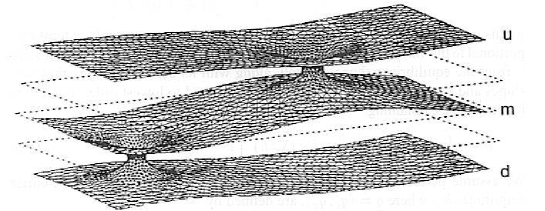
Figure 26: Example of a structure with $M=3$ membranes and $N=2$ necks connecting them. Periodic boundary conditions are understood. From X. Michalet, D. Bensimon, B. Fourcade, Phys. Rev. Lett. 72 168 (1994).

In the limit where $M\to\infty$ and $N\to\infty$ one recovers the sponge phase.

We have thus seen that the intimations of the Helfrich hamiltonian on vesicle shapes, even at the mean field level, reveal an unsuspected richness.

5 Shape fluctuations in vesicles

Red blood cells suspended in solution exhibit a remarkable flicker phenomenon, which is best seen with a phase contrast microscope and appears as a shimmering at the junction of the rim and the center of the cells. The origin of this phenomenon was debated since its first observation in 1890 [12] and until the quantitative analysis by Brochard and Lennon [11] proved beyond doubt that it was due to Brownian motion. The intensity of the phenomenon is due to the fact that the surface tension vanishes.

Indeed, let us estimate the amplitude of shape fluctuations in a membrane described by the Helfrich hamiltonian. We assume that the equilibrium shape of the membrane is planar, and we take its plane to be the $(x,y)$ plane. We represent the shape of the membrane in the Monge form, i.e., by giving the third coordinate $z,$ as a function of the other two:

$$z=h(x,y).$$ (5.1)

We set $\underline{\sigma}=(x,y).$ The hamiltonian then takes the form:

$$F=\int{\rm d}^{2}\underline{\sigma}\sqrt{1+\left(\nabla h\right)^{2}}\left[\gamma+\frac{1}{2}\kappa\left(\nabla\cdot\frac{\nabla h}{\sqrt{1+\left(\nabla h\right)^{2}}}\right)^{2}\right].$$ (5.2)

In this equation $\nabla$ denotes the two-dimensional nabla operator, and the term proportional to the Gaussian curvature is understood. We assume that the deformation $h$ from the equilibrium shape is small, along with its derivatives: i.e., that both slopes and curvatures are small. We can then expand to lowest order in $h$ and in its derivatives, obtaining

$$F\simeq\int{\rm d}^{2}\underline{\sigma}\left[\frac{1}{2}\gamma\left(\nabla h\right)^{2}+\frac{1}{2}\kappa\left(\nabla^{2}h\right)^{2}\right].$$ (5.3)

We assume periodic boundary conditions on a square of side $L$. The Fourier amplitudes $h_{\underline{q}},$ where $\underline{q}=(q_{x},q_{y}),$ are defined by

$$h_{\underline{q}}=\int{\rm d}^{2}\underline{q}{\rm e}^{{\rm i}\underline{q}\cdot\underline{\sigma}}h({\underline{\sigma}}).$$ (5.4)

In terms of these amplitudes, the Helfrich hamiltonian becomes

$$F=\frac{1}{2L^{2}}\sum_{\underline{q}}\left[\gamma q^{2}+\kappa q^{4}\right]\left|h_{\underline{q}}\right|^{2}.$$ (5.5)

By the equipartition theorem we have

$$\left<\left|h_{\underline{q}}\right|^{2}\right>=L^{2}\frac{k_{\rm B}T}{\gamma q^{2}+\kappa q^{4}}.$$ (5.6)

We see that, if the surface tension vanishes, the fluctuation amplitude diverges, at small $q,$ like $q^{-4}.$ The finite size of the membrane imposes a low $q$ cutoff at $\pi/L.$ We can then integrate the former expression to get an estimate of the fluctuation amplitude:

$$\left<h^{2}\right>=\frac{1}{(2\pi)^{2}L^{2}}\int_{\pi/L}^{\infty}{\rm d}^{2}\underline{q}\left<\left|h_{\underline{q}}\right|^{2}\right>=L^{2}\frac{k_{\rm B}T}{4\pi^{3}\kappa}.$$ (5.7)

The square amplitude diverges like $L^{2}$. If the surface tension had not vanished, we would have had a much weaker (logarithmic) divergence. As an order of magnitude, since $\kappa\sim 10^{-19}$–$10^{-20}\,{\rm J}$, taking $L\sim 8\mu{\rm m}$ as for human red blood cells, we obtain $\sqrt{\left<h^{2}\right>}\sim 0.4$–$0.7\,\mu{\rm m}.$

More generally, let us consider the fluctuations of a $D$-dimensional surface in the Monge representation, governed by a generic Hamiltonian of the form

$${\cal H}\propto\int{\rm d}^{D}\underline{\sigma}\left(\nabla^{\omega}h\right)^{2}.$$ (5.8)

For the case of the rigidity-dominated membranes we have $\omega=2,$ whereas for the case of an ordinary interface with a nonvanishing surface tension we would have $\omega=1.$ The wandering exponent $\zeta$ describes the behavior of the excursions of the membrane as a function of its lateral size $\left<h^{2}\right>\propto L^{2\zeta}$ or, equivalently, the behavior of the height-height correlation function:

$$\left<\left(h(0)-h(\underline{\sigma})\right)^{2}\right>\propto\left|\underline{\sigma}\right|^{2\zeta}.$$ (5.9)

We obtain

$$\zeta=\frac{1}{2}\left(2\omega-D\right).$$ (5.10)

We obtain therefore $\zeta=1$ for the case of membranes (whereas $\zeta=0$ for interfaces with nonvanishing surface tension), which implies that the aspect ratio of the fluctuations over lateral size does not decrease with increasing size. This means that membranes should appear “wobbled” in the same way even at the largest scales. As we shall see, the situation is even worse.

Helfrich [58] recognized the important effects of membrane fluctuations. On the one hand, the projected area $A_{\rm p}$ of the membrane is reduced with respect to its true area $A$ (see eq. (5.37) below). Moreover, the wandering of the membrane from its equilibrium configuration implies the existence of a long-range repulsion between undulating membranes, as it had already been pointed out in 1978 by Helfrich [56]. To fix one’s ideas, let us consider a membrane constrained by two parallel, planar walls, set at a distance $2d$ apart. The membrane is on average in the middle, but it collides with either wall from time to time. Collisions are separated by a typical length $L_{\rm coll}\sim d^{1/\zeta},$ where $\zeta$ is the wandering exponent. Therefore the free energy per unit area will have a repulsive contribution proportional to the density of the collisions, i.e., to $L_{\rm coll}^{-D}\sim d^{-D/\zeta}.$ This “steric repulsion” term decreases like $d^{-2}$ for membranes, i.e., just like the van der Waals attraction at short distances. One can thus expect in principles regimes in which van der Waals forces dominate, and parallel membranes are bound to each other, or in which steric repulsion dominates, and they repel each other. The transition between the two regimes is called unbinding: although it is not described by this simple argument, as we shall see later, it has been observed in actual membranes. Finally, he recognized that the rigidity modulus $\kappa$ itself is renormalized by the fluctuations, and becomes smaller and smaller for larger and larger membranes [58].

A more rigorous analysis of shape fluctuations in vesicles requires one to take into account the fact that the equilibrium shape is not planar. The necessary techniques were developed by Peterson [97]. These techniques have been recently applied to a reappraisal of the flicker phenomenon in red blood cells by Peterson, Strey, and Sackmann [98]. In general one would like to compute the variation of the elastic free energy $F$ under a slight deformation of the vesicle shape, starting from a reference equilibrium shape $S_{0}.$ It is assumed that the deformation satisfies the constraints that define the ensemble. There are many ways to parametrize the deformation: the most convenient choice is the normal gauge, in which the deformation is described by the distance $h$ of the deformed surface $S$ from the reference one $S_{0},$ measured along the normal to $S_{0}$ at each point. One then computes the variation of $F$ to second order in the deformation:

$$\delta^{2}F[h]=\frac{1}{2}\int{\rm d}\underline{\sigma}{\rm d}\underline{\sigma}^{\prime}\left.\frac{\delta^{2}F}{\delta h(\underline{\sigma})\delta h(\underline{\sigma}^{\prime})}\right|_{h=0}h(\underline{\sigma})h(\underline{\sigma}^{\prime}).$$ (5.11)

The probability of a given deformation is proportional, in the Gaussian approximation, to $\exp[-\delta^{2}F/k_{\rm B}T].$ The constraints can be taken into account in the following way. The deformation $h$ is splitted into a first-order term $h_{1},$ which satisfies the constraints to first order, and a second-order term $h_{2},$ which is chosen to enforce the constraints to second order. The first-order term $h_{1}$ parametrizes the deformation, whereas the variation of the elastic energy is given by the second-order variation of $F$ times $h_{1}^{2}$ plus the first order variation multiplied by the second-order term $h_{2}.$ Equivalently, one may consider adjusting the Lagrange multipliers in order to keep the constraints satisfied to second order.

Once the quadratic variation $\delta^{2}F$ of $F$ is obtained, one diagonalizes it by taking advantage of its symmetries: in the case of the red blood cells, the axial symmetry and the up-down symmetry. It is an extremely stringent check on the calculation that all the rigid Euclidean motions emerge as zero energy modes. The amplitudes of the fluctuating modes are obtained from the equipartition theorem, and are then summed up to obtain the fluctuation profile. Since one cannot rule out in principle the existence of a shear elasticity modulus $\mu$ in red blood cells, due to the loose ankyrin-spectrin network present on the interior of the membrane, the formalism requires a slight generalization [97, 98]. The fluctuation profile then depends on the dimensionless parameter $\epsilon=\mu R_{0}^{2}/\kappa.$ In fig. 27 the thickness fluctuation profile is shown as a function of this parameter.

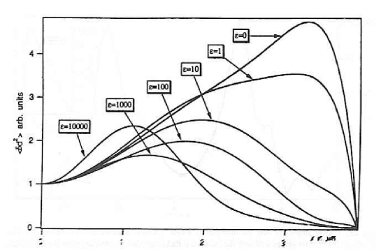
Figure 27: Thickness fluctuation profile for various values of the ratio $\epsilon=\mu R^{2}_{0}/\kappa.$ From M. A. Peterson, H. Strey, E. Sackmann, J. Phys. II France 2 1273 (1992).

We see that, as the shear elasticity is reduced, the fluctuation maximum moves toward the rim. At small values of the shear modulus, this effect is more pronounced in the BC model than in the SC model. Experimental results are shown in fig. 28. They are compatible with a very small value of the shear modulus $\mu,$ with the predictions of the BC model, and with a value of $\kappa=1.4\times 10^{-19}$ J. This value is of the order of that of pure lipid bilayers [37], but a factor two smaller than that of a mixture of a physiological lipid and cholesterol [37, 39]. It is possible that the discrepancy is due to the presence of small proteins [77], since red blood cell membranes contain about 50% proteins by weight, covering about 20% of the area.

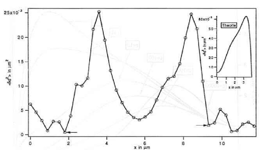
Figure 28: Flicker amplitude over the diameter of a cell. (Arrows indicate the cell boundary.) The observed distribution agrees well with the theoretical flicker amplitudes obtained from the BC model. From M. A. Peterson, H. Strey, E. Sackmann, J. Phys. II France 2 1273 (1992).

In order to be able to go beyond the Gaussian approximation, we now need to pay a closer look at fluctuations. The most convenient framework introduces the effective potential $\Gamma[\vec{r}_{0}]$ and the renormalization group [95, 73, 28, 52]. Let us consider an fluctuating membrane, whose instantaneous configuration is parametrically represented by $\vec{r}=\vec{r}(\underline{\sigma}),$ $\vec{r}\in{\bf R}^{d}$ and $\underline{\sigma}\in{\bf R}^{2}.$ The free energy ${\cal F}$ of the membrane is given in terms of the partition function

$${\cal F}=-k_{\rm B}T\log\int{\cal D}\vec{r}\exp\left\{-\frac{F[\vec{r}]}{k_{\rm B}T}\right\},$$ (5.12)

where $F[\vec{r}]$ is the Helfrich hamiltonian

$$F=\oint_{S}{\rm d}A\left[\tau_{0}+\frac{\kappa_{0}}{2}H^{2}+\overline{\kappa}_{0}K\right].$$ (5.13)

If we want to assign the membrane a given average shape $\vec{r}_{0}(\underline{\sigma}),$ we can introduce a fictitious external field $\vec{\lambda},$ coupling to the position $\vec{r},$ such that $\left<\vec{r}(\underline{\sigma})\right>_{\lambda}=\vec{r}_{0}(\underline{\sigma}).$ The effective potential $\Gamma[\vec{r}_{0}]$ is the defined as the Legendre transform of ${\cal F}$ with respect to $\lambda$:

$$\Gamma[\vec{r}_{0}]={\cal F}-\int{\rm d}A\,\vec{\lambda}\cdot\vec{r}_{0}(\underline{\sigma}).$$ (5.14)

(A precise definition needs to take into account reparametrization invariance.)

Euclidean and reparametrization invariances dictate the form of the effective potential, just as they do for the Helfrich hamiltonian [95]. Therefore

$$\Gamma[\vec{r}_{0}]=\int{\rm d}\bar{A}\left[\tau_{\rm eff}+\frac{\kappa_{\rm eff}}{2}\bar{H}^{2}+\overline{\kappa}_{\rm eff}\bar{K}+\ldots\right],$$ (5.15)

where $\bar{A}$ is the area element of the average membrane shape, and $\bar{H},$ $\bar{K}$ its curvatures. In this formula we have neglected terms which depend on higher derivatives of the average shape. This expression defines the effective parameters $\tau_{\rm eff},$ $\kappa_{{\rm eff}}$ and $\overline{\kappa}_{{\rm eff}}.$ If the equilibrium shape is flat, all curvature terms vanish at equilibrium, so that

$$\Gamma_{\rm eq}=\tau_{\rm eff}A_{\rm p}.$$ (5.16)

Therefore $\tau_{\rm eff}$ is the effective frame tension of the membrane.

Now, the effective frame tension $\tau_{\rm eff},$ must be equal to the “$q^{2}$ coefficient,” $\gamma,$ of the two-point height correlation function of the membrane, defined by

$$\left<|h_{\underline{q}}|^{2}\right>=\frac{1}{\gamma q^{2}+O(q^{4})}.$$ (5.17)

It is sufficient to recall that the effective potential $\Gamma$ is also the generating functional of the vertices, and in particular its second derivative yields the inverse of the propagator. By going over to the Monge representation of $\vec{r}_{0}$ we obtain

$$\left<|h_{\underline{q}}|^{2}\right>^{-1}=\left.\frac{\delta^{2}\Gamma}{\delta h_{-\underline{q}}\delta h_{\underline{q}}}\right|_{h=0}.$$ (5.18)

We obtain therefore $\gamma=\tau_{\rm eff}.$ In a similar way, the effective rigidity $\kappa_{\rm eff}$ can be related to the coefficient of $\left(\nabla^{2}\bar{h}\right)^{2}$ in the effective potential.

If we wish to investigate the behavior of the membrane at larger and larger distances, we can apply the renormalization group approach. The effective Wilson hamiltonian ${\cal H}_{\rm eff}(s)$ is obtained by integrating out all fluctuations whose wavenumbers $\underline{q}$ are contained in a shell $\Lambda/s<\left|\underline{q}\right|<\Lambda,$ where $s>1.$ Again by Euclidean symmetry, ${\cal H}_{\rm eff}(s)$ can be expanded in the form

$${\cal H}_{\rm eff}(s)=\int{\rm d}A\left[\tau_{\rm eff}(s)+\frac{\kappa_{\rm eff}(s)}{2}H^{2}+\overline{\kappa}_{\rm eff}(s)K+\ldots\right].$$ (5.19)

We then rescale the lengths in order to bring the upper cutoff back to $\Lambda$:

$$\vec{r}\to s\,\vec{r},\qquad\underline{q}\to s^{-1}\underline{q},$$ (5.20)

yielding the renormalized Hamiltonian

$${\cal H}(s)=\int{\rm d}A\left[\tau(s)+\frac{\kappa(s)}{2}H^{2}+\overline{\kappa}(s)K+\ldots\right].$$ (5.21)

Since the “order parameter” in our case is the length $h,$ there is no need of the additional “wavefunction” rescaling, which usually appears in critical phenomena. The relation between the effective parameters and the renormalized ones is simply

$$\kappa(s)=\kappa_{\rm eff}(s);\qquad\overline{\kappa}(s)=\overline{\kappa}_{\rm eff}(s);\qquad\tau(s)=s^{2}\tau_{\rm eff}(s).$$ (5.22)

The renormalized parameters are actually computed by integrating the renormalization flow equations, which are obtained by considering $s=1+\epsilon,$ where $\epsilon$ is infinitesimal. By the definitions of the effective potential $\Gamma$ and of the effective Wilson hamiltonian ${\cal H}_{\rm eff}(s)$ it is clear that

$$\lim_{s\to\infty}{\cal H}_{\rm eff}(s)=\Gamma.$$ (5.23)

Now, if we are considering an ensemble in which the total area $A$ of the membrane fluctuates and a frame tension $\tau$ is applied to it, we have to choose the initial condition $(\gamma_{0},\kappa_{0},\overline{\kappa}_{0})$ of the renormalization trajectory in such a way that

$$\lim_{s\to\infty}\tau_{\rm eff}(s)=\tau.$$ (5.24)

We see therefore that the essential step of the renormalization group calculation is the evaluation of ${\cal H}_{\rm eff}(s),$ where $s=1+\epsilon.$ This is quite similar to the calculation of the effective potential, only that one restricts the wavenumbers $\underline{q}$ of the fluctuations to be integrated out to the shell $\Lambda/s<|q|<\Lambda.$ This calculation can be performed perturbatively. One chooses as a reference configuration the equilibrium one $\vec{r}_{0}$ and expands in the small (normal) deformation field $\vec{h}=\vec{r}-\vec{r}_{0}.$ The effective Wilson hamiltonian ${\cal H}_{\rm eff}(s)$ can be then expanded in powers of the temperature:

$${\cal H}_{\rm eff}(s)=\sum_{\ell}{\cal H}_{\rm eff}^{\ell}(s)\left(k_{\rm\beta}T\right)^{\ell}.$$ (5.25)

If one stops at one loop level, it is sufficient to consider only the second variation $\delta^{2}$ of the Helfrich hamiltonian with respect to the deformation field $\vec{h}=\vec{r}-\vec{r}_{0}.$ The result reads

$${\cal H}_{\rm eff}(s)=F[\vec{r}_{0}]-k_{\rm B}T\log\int_{s}{\cal D}\vec{h}\exp\left(-\frac{\delta^{2}F}{k_{\rm B}T}\right).$$ (5.26)

The notation $\int_{s}$ reminds the constraint on the fluctuations.

The measure factor ${\cal D}\vec{h}$ has to be considered with somecare [28, 52, 31, 13], and has been discussed in the seminar by Thomas Powers in this School [103]. In principle it contains two contributions: one (known as the Faddeev-Popov determinant) which takes into account the volume occupied by different reparametrizations of the same surface. It is defined and discussed in Appendix B. The other (discussed in particular in refs. [13, 103]), which takes into account the fact that the actual number of degrees of freedom involved in the fluctuating surface is proportional to the number of molecules, i.e., to the actual area element ${\rm d}A$. It turns out, however, that one can simplify the problem (to the level of not worrying at all about these contributions) if one works in the normal gauge.

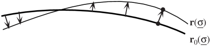
Figure 29: Definition of the normal gauge. Given a reference shape represented as $\vec{r}_{0}(\underline{\sigma}),$ the deformation is represented by the displacement $\vec{h}=\vec{r}(\underline{\sigma})-\vec{r}_{0}(\underline{\sigma})$ along the normal to the reference shape.

We consider momentarily membranes embedded in $d$-dimensional space. Let the reference shape be parametrically represented by $\vec{r}_{0}=\vec{r}_{0}(\underline{\sigma}),$ where $\vec{r}_{0}\in{\bf R}^{d}.$ The instantaneous shape of the membrane is represented by $\vec{r}=\vec{r}(\underline{\sigma}).$ In the normal gauge one imposes the condition

$$\left(\vec{r}(\underline{\sigma})-\vec{r}_{0}(\underline{\sigma})\right)\cdot\partial_{i}\vec{r}_{0}(\underline{\sigma})=0,\qquad i=1,2.$$ (5.27)

The displacement $\vec{h}(\underline{\sigma})=\vec{r}(\underline{\sigma})-\vec{r}_{0}(\underline{\sigma})$ has therefore $d-2$ independent components. In the normal gauge the Faddeev-Popov determinant $\Delta_{\rm FP}$ turns out to be local and to contribute only a (divergent) shift to the effective membrane tension $\gamma.$

The calculation of the renormalization group flow to one loop is reported in Appendix C. The result is the following [58, 95, 73, 31]:

$$s\frac{\partial\kappa(s)}{\partial s} = -\frac{3}{4\pi}\frac{k_{\rm B}T}{1+\tau(s)/\kappa\Lambda^{2}},$$ (5.28)

$$s\frac{\partial\overline{\kappa}(s)}{\partial s} = \frac{5}{6\pi}\frac{k_{\rm B}T}{1+\tau(s)/\kappa\Lambda^{2}},$$ (5.29)

$$s\frac{\partial\tau(s)}{\partial s} = 2\tau(s)+\frac{\Lambda^{2}}{4\pi}k_{\rm B}T\log\left(\frac{\kappa+\tau(s)/\Lambda^{2}}{k_{\rm B}T}\right).$$ (5.30)

The calculation is valid to one loop, hence it only holds if the terms of order $k_{\rm B}T$ are small. This implies either $\kappa>k_{\rm B}T$ or $\tau/\Lambda^{2}>k_{\rm B}T.$ Let us remark that these equations imply that the bending rigidity $\kappa$ decreases when one goes to larger and larger scales: the membrane becomes more and more crumpled. On the other hand, the Gaussian rigidity $\overline{\kappa}$ increases: although this has no effect on the behavior of an isolated membrane (whose topology is fixed), it is important as one considers ensembles of fluctuating membranes, as we shall do in the next section.

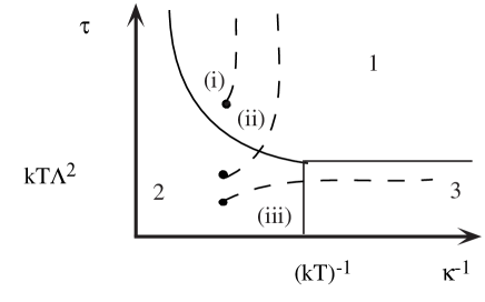
Figure 30: Different behaviors of fluid membranes with respect to fluctuations in the $(\tau,\kappa^{-1})$ plane. 1: Tension-dominated region. 2: Rigidity-dominated region. 3: Fluctuation-dominated region. Also shown are the renormalization trajectories (i)–(iii) discussed below.

This perturbative result allows us to define three different regions characterizing the fluctuations of fluid membranes:

1. Tension-dominated region:

   $$\tau>\kappa\Lambda^{2};\qquad\tau>k_{\rm B}T\Lambda^{2}.$$ (5.31)

   In this region the fluctuations are small and governed by tension $\tau$ (“drumhead model”). The flow equations can be approximated by

   $$s\frac{\partial\kappa}{\partial s}=s\frac{\partial\bar{\kappa}}{\partial s}=0;\qquad s\frac{\partial\tau}{\partial s}=2\tau.$$ (5.32)

2. Rigidity dominated region:

   $$\kappa>k_{\rm B}T;\qquad\tau<\kappa\Lambda^{2}.$$ (5.33)

   In this region fluctuations are small, but are dominated by the rigidity term. One has the following approximate flow equations:

   $$s\frac{\partial\kappa}{\partial s} = -\frac{3k_{\rm B}T}{4\pi},$$ (5.34)

   $$s\frac{\partial\bar{\kappa}}{\partial s} = \frac{5k_{\rm B}T}{6\pi},$$ (5.35)

   $$s\frac{\partial\tau}{\partial s} = \tau\left(2+\frac{k_{\rm B}T}{4\pi\kappa}\right).$$ (5.36)

   The renormalization of the surface term can be attributed to an increase of the ratio total area/projected area due to thermal fluctuations. Indeed, to leading order in $k_{\rm B}T$ this ratio is given by

   $$\frac{\left<A\right>}{A_{\rm p}}=1+\frac{k_{\rm B}T}{4\pi\kappa}\log A_{\rm p}.$$ (5.37)

3. Thermal fluctuations dominated region:

   $$\kappa<k_{\rm B}T;\qquad\tau<k_{\rm B}T\Lambda^{2}.$$ (5.38)

   In this domain perturbation theory breaks down: one expects that steric interactions and topology changes become important.

As one considers the same membrane at increasing length scale $\ell,$ the renormalization group flows will carry one from one region to another. One can find different kinds of trajectories. Starting from a given value $\kappa_{0}>k_{\rm B}T$ of the rigidity one can have:

• If the surface tension $\tau_{0}$ is large enough, the trajectory remains in the tension-dominated region at all scales, and is described by the simple drumhead model like an ordinary interface, with rigidity-induced corrections with the fixed rigidity $\kappa_{0}$.

• For smaller surface tensions, one may cross over from the rigidity-dominated region to the tension-dominated region: it exists therefore a crossover length $\ell_{\rm c}$ such that for $\ell>\ell_{\rm c}$ one is in the tension-dominated regime with some (nonzero) effective tension $\tau_{\rm eff}$ and an effective rigidity $\kappa_{\rm eff}.$ The crossover length $\ell_{\rm c}$ will be given by

  $$\ell_{\rm c}=\sqrt{\frac{\kappa_{\rm eff}}{\tau_{\rm eff}}}.$$ (5.39)

  For $\ell<\ell_{\rm c}$ one is in the rigidity-dominated regime: tension effects can be neglected, and the effective rigidity depends on the scale $\ell$:

  $$\kappa(\ell)=\kappa_{0}-\frac{3k_{\rm B}T}{4\pi}\log\left(\frac{\ell}{\ell_{0}}\right),$$ (5.40)

  where $\ell_{0}$ is the molecular size.

• If the tension is too small, there is a length scale $\ell_{\rm c}$ in which one crosses over to the fluctuation-dominated regime and the model breaks down. This length can be defined by the condition that $\kappa(\ell_{\rm c}),$ as defined by eq. (5.40), is of order $k_{\rm B}T.$ This length is known as the persistence length [45] and depends exponentially on the rigidity $\kappa_{0}$:

  $$\ell_{\rm c}=\xi\simeq\ell_{0}\exp\left(\frac{4\pi\kappa_{0}}{3k_{\rm B}T}\right).$$ (5.41)

  At larger scales the membrane will be crumpled, with a correlation length for its normals of the order of $\xi.$

François David and Emmanuel Guitter [27, 30] have considered the model with bending rigidity in the large $d$ limit. The results can be described as a phase diagram in the tension-rigidity plane. For sufficiently large surface tension $\tau,$ the system is in a “flat” phase with a finite ratio of the projected area to the total area. As one approaches a critical line $\tau_{\rm c}(\kappa_{0}),$ this ratio vanishes: on the other side of this line the surface is crumpled and the system does not exist—unless one takes into account steric interactions and topology changes. Along the critical line the frame tension remains finite. However, even before reaching the critical line, the system becomes instable with respect to nonhomogeneous fluctuations. As one reaches the transition line, the frame tension remains finite.

The effective model describing the membrane at long distances is the Liouville action model [100], introduced by Polyakov in the context of strings. It describes a Gaussian surface (defined by the vector field $\vec{r}$), coupled to a fluctuating intrinsic metric $g_{ij}.$ We discuss it briefly in Appendix D. It is usually believed that this model also applies to membranes embedded in finite-dimensional spaces. However, in this case, self-avoiding effect are probably essential in determining the actual behavior of the membrane. Moreover, it is generally believed [36] that these membranes should assume configurations characteristic of branched polymers. Since this is a nonperturbative effect, it is rather difficult to study it analytically. Cates [18] argues that it is related to an instability of the Liouville field theory with respect to the formation of “spikes”.

A way to control this instability in closed vesicles is to introduce osmotic pressure. Leibler, Singh and Fisher [79] verified by numerical studies that two-dimensional self-avoiding vesicles change continuously from a deflated state with the characteristics of branched polymers to an inflated state as the osmotic pressure $p$ is increased. This transition has been further studied by real-space renormalization group techniques [2] and by conformal group techniques [17], which have allowed to determine its critical exponents in 2-D. There have been fewer studies of the corresponding transition in 3-D. In particular, Gompper and Kroll [50] and Baumgärtner [3] have numerically shown that the deflated-inflated transition is first-order in 3-D. A finite-size scaling analysis of the deflation-inflation transition has been recently performed by Damman et al. [26].

I close this section by pointing out that the fact that the effective rigidity decreases at larger and larger length scales can be interpreted in terms of the Mermin-Wagner theorem [83], which states that a continuous symmetry cannot be spontaneously broken in two dimensions by a local Hamiltonian. In our case the continuous symmetry is the Euclidean one, which would be broken for our two-dimensional membranes if they exhibited a flat phase.

6 Interacting fluid membranes

We now consider an ensemble of fluctuating, self-avoiding membranes, following Huse and Leibler [65]. The effects of excluded volume and of the topological term $\overline{\kappa}\int{\rm d}A\,K$ are essential. We shall first go across the phase diagram, and identify the phases which may be present. We shall then examine each of them more closely.

Let us first set $\overline{\kappa}=0,$ thus effectively neglecting the topological term but allowing for changes in topology.

From a physical point of view, we are considering a solution of amphiphile in water. We assume for the time being that the bending rigidity $\kappa_{0}$ is quite large, and neglect momentarily renormalization effects. The “bare” surface tension $\tau_{0}$ appearing in the Helfrich hamiltonian is proportional to the chemical potential of the amphiphile. It can be controlled by changing the amphiphile concentration $\phi.$ For $\tau_{0}$ large and positive, i.e., for a small concentration $\phi$ of the amphiphile, the membrane breaks down into small isolated vesicles: as a consequence, the volume is separated into two components: one inside and one outside of the droplets. We can assign “spins” to each component (e.g., “down” inside and “up” outside) and we recognize a spontaneous symmetry breaking between the two components.

In principle, we could imagine to force the spins to be up on one side of the sample, and down on the other side. In this case there should be a membrane running across the sample, costing a free energy proportional to its section. In this phase, therefore, there is a nonzero surface tension $\tau$ for the membrane at a macroscopic level: Huse and Leibler [65] call it the tense droplet phase.

Increasing the amphiphile concentration (reducing $\tau_{0}$) the volume enclosed by the droplets increases. The membranes come closer to one another and are likely to form “necks” in order to increase entropy. Therefore the region of minority spins becomes connected over longer and longer distances. Well before reaching a volume fraction equal to one half, the connected regions can percolate. We thus have two infinite connected regions of unequal size. We have obtained a bicontinuous phase. The symmetry between inside and outside is still broken. Therefore there will still be a nonzero macroscopic surface tension $\tau$ between a prevalently “up” and a prevalently “down” region. The phase can therefore be called tense bicontinuous.

If $\tau_{0}$ is further reduced, the symmetry should eventually be restored. We thus obtain an isotropic random phase. This phase is analogous to the disordered phase of a ferromagnet, whereas the tense phase is analogous to the ordered one. The spin-up spin-down symmetry can be explicitly broken by introducing a spontaneous curvature $H_{0}$, or a “magnetic field” $\mu$ coupling to the spins. The transition from the tense bicontinuous to the random isotropic phase should be critical at the symmetry point ($H_{0}=\mu=0$) and belong to the Ising universality class. Both phases are also called “sponge” phases in the recent literature. In particular, the tense bicountinuous phase is called the asymmetric sponge, whereas the random isotropic is called the symmetric sponge. They are usually identified with the shear birifringent L₃ phase observed in some ternary (and also binary) mixtures.

The tense bicountinuous phase is “paradoxical”: the broken symmetry is not observable. In principle, we could have two identical-looking samples belonging to different phases, and one could notice this fact only by observing the interface which forms when the two are put in contact. Something similar happens in antiferromagnets: the order parameter of an antiferromagnet has a free choice, but it is not possible to distinguish between samples corresponding to different values of it. In principle, if one puts them in contact, one should observe an interface: in practice, we can probe its order only indirectly.

Let us now go all the way to a high concentration of amphiphile. Having to accommodate a large amount of membranes, which refuse to cross and pay energy to bend, the most likely organization is to pack them into stacks. The membranes are called lamellae in this context, and this phase is called the lamellar phase. From the symmetry point of view it is a (lyotropic) smectic A phase, and it is characterized by quasi-long range order in the positions of the lamellae, and long-range order in their orientations. The lamellae lie on parallel planes, on average, in different regions of the sample. On the other hand, the concentration-concentration correlation function of the amphiphile decays (like a power law) to an average value instead of keeping the rippled behavior characteristic of the lamellar organization at short distances.

The quasi-long range positional order can be destroyed by a defect-unbinding mechanism not unlike that underlying the Kosterlitz-Thouless transition. One thus goes over to a nematic phase, characterized by exponential decay of the concentration-concentration correlations (and therefore macroscopically homogeneous), but with long-range orientational order. Microscopically, the difference between the lamellar (smectic) and the nematic phase lies in the presence of unbound defects. There may be actually different kinds of defects. The bilayer may end at a free edge, or three bilayers meet on one line (seams), as shown in fig. 31.

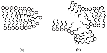
Figure 31: Examples of defects in lamellar phases: (a) edges; (b) seams. These defects are assumed to be forbidden in the simplified model of interacting fluid membranes.

In both cases, by going around the dislocation, the number of lamellae increases or decreases by one. On the other hand one may have an edge dislocation, where one lamella bends on itself, as in fig. 32, or a more complicated screw dislocation, but with a mismatch of two in lamella number.

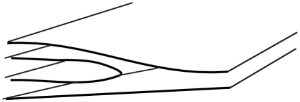
Figure 32: An edge dislocation which does not break “spin” ordering in lamellar phases.

These defects may also interfere with the “spin” order of the solvent. In a perfect lamellar phase, it is possible to assign to regions occupied by the solvent a spin, such that regions separated by a membrane have opposite spin. This is not possible if the membrane possesses free edges or seams. However, if these defects remain at a microscopical scale, this is still possible to define an ideal surface which spans the defect, and the macroscopical “spin” order is not disrupted. With the proliferation of defects, one reaches the point in which there is no macroscopically acceptable assignment of spins. In this case, spin symmetry is restored. On the other hand also the orientational order characteristic of the nematic phase will eventually undergo a transition (of the Heisenberg universality class). These considerations make it plausible that at a sufficiently high temperature (or rather, small bending rigidity $\kappa$) the nematic phase will leave the place to an isotropic phase, which we can identify with the random, isotropic phase discussed above.

The frontiers between the different phases should correspond to renormalization group trajectories. In the large rigidity region, we have seen that the renormalization group trajectories are given by

$$s\frac{\partial\kappa}{\partial s} = -\frac{3k_{\rm B}T}{4\pi},$$ (6.1)

$$s\frac{\partial\tau}{\partial s} = \tau\left(2+\frac{4k_{\rm B}T}{4\pi\kappa}\right).$$ (6.2)

Therefore, defining $\beta=k_{\rm B}T/\kappa,$ we have $\Delta\tau\sim s^{2+O(\beta)},$ while $\Delta\beta\sim\log s.$ We thus expect the trajectories to have the form

$$\tau\propto\exp\left(-\frac{8\pi\kappa}{k_{\rm B}T}\right).$$ (6.3)

The resulting phase diagram in the $(\kappa^{-1},\tau)$ plane at $\overline{\kappa}=0$ is drawn in fig. 33.

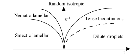
Figure 33: Phase diagram for fluctuating membranes at $\overline{\kappa}=0.$ The percolation transition between the dilute droplets and the tense bicontinuous phase does not correspond to a thermodynamic singularity. From D. Huse, S. Leibler, J. Phys. France 49 605 (1988).

Let us now consider the effects of the gaussian rigidity $\overline{\kappa},$ neglecting for the time being its renormalization. From the Gauss-Bonnet theorem we know that the integral over the surface of the Gaussian curvature $K$ is related to the number $n_{\rm c}$ of connected surface components and to the number $n_{\rm h}$ of handles:

$$\int{\rm d}AK=4\pi(n_{\rm c}-n_{\rm h}).$$ (6.4)

Let us keep a large value of the bending rigidity $\kappa.$ If we let $\overline{\kappa}$ become large and positive, structures with many handles will be favored: these structures can be built up with minimal surfaces, in which the mean curvature locally vanishes. Therefore, for both $\overline{\kappa}$ and $\kappa$ large and positive, we expect the formation of regular structures, made of minimal or almost minimal surfaces, with a great number of handles. These structures are collectively known as “plumber’s nightmares”, since they represent a pipework in which one does not know whether one is in the interior or in the exterior. An example of such structures is shown in fig. 34.

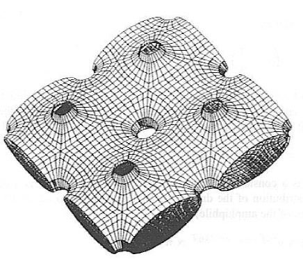
Figure 34: An example of a plumber’s nightmare structure. From D. Huse, S. Leibler, J. Phys. France 49 605 (1988).

If we go on the other side, towards large negative values of $\overline{\kappa},$ the formation of disconnected components will be favored. This can take place in the presence of a rather large concentration of amphiphile. One will observe a large concentration of droplets, which, because of their steric repulsion, will probably tend to organize in a close-packed droplet crystal.

Summing up these considerations, we obtain the phase diagram in the $(\tau,\overline{\kappa})$-plane, assuming a large value of the bending rigidity $\kappa,$ and neglecting for the time being the possible occurrence of free edges and seams, and their effects. The diagram is shown in fig. 35. Along the $\overline{\kappa}=0$ axis we recover the sequence of phases we had described before.

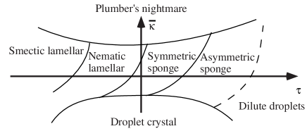
Figure 35: Phase diagram of an ensemble of nonintersecting membranes in the $(\tau,\overline{\kappa})$-plane, for fixed $\kappa\gg k_{\rm B}T.$ From D. Huse, S. Leibler, J. Phys. France 49 605 (1988).

We now discuss each of the phases in detail, and take into account the controversial consequences of defects and fluctuations.

Droplet phase

As I have mentioned above, amphiphilic vesicles are usually formed by sonication and are not assumed to be in equilibrium in usual conditions. However, there have been recently observations of droplet phases apparently at equilibrium in binary [15, 16] as well as in more complicated systems [62, 63, 61]. This phase has been named L${}_{4}.$ Experimentally, it appears in a very narrow region of the phase diagram, or with a rather special amphiphile in the case of the binary mixture.

In the equilibrium droplet phase one should observe a large polydispersity of droplet size. If one neglects the fluctuations, the elastic energy of a spherical droplet is given by

$$E_{\rm d}=8\pi\left(\kappa+\frac{\overline{\kappa}}{2}\right),$$ (6.5)

independent of its size. Because of this scale invariance, logarithmic corrections to the free energy of the droplet (which are usually neglected in the thermodynamic limit) become very important. One obtains an expression of the form

$$F_{\rm d}(n)=\alpha_{\rm d}k_{\rm B}T\ln n+F_{0},$$ (6.6)

where $F_{0}$ is a constant, and $\alpha_{\rm d}$ is a universal coefficient. As a consequence, the size distribution of the droplets becomes (taking into account the chemical potential, $\mu,$ of the amphiphile)

$$\rho_{\rm d}(n)\propto\mathop{\rm e}\nolimits^{-(F_{\rm d}(n)-\mu n)/k_{\rm B}T}\propto n^{-\alpha_{\rm d}}\mathop{\rm e}\nolimits^{-n/n^{*}},$$ (6.7)

where $n^{*}=k_{\rm B}T/|\mu|$ is a characteristic size, dictated by the amphiphile concentration. Of course, this form can only hold for $n>n_{\rm c},$ where $n_{\rm c}$ is the minimum number of amphiphilic molecules necessary to make a droplet.

The form (6.6) was first proposed by Helfrich [59]. It has been reexamined by Huse and Leibler [65], Simons and Cates [110], and more recently by Morse and Milner [90]. The contributions proportional to $\ln n$ arise from the renormalization of the elastic constant which we have mentioned before, but also by the reduction in the translational and undulational degrees of freedom, which depend on droplet size. The authors do not agree on the value of $\alpha_{\rm d}$. Part of the disagreement arises from a controversy over the coefficients, $\alpha_{\kappa}$ and $\alpha_{\overline{\kappa}},$ which appear in the renormalization of the bending constants. In the previous section, I have reported the most widely accepted results, namely $\alpha_{\kappa}=-3$ and $\alpha_{\overline{\kappa}}=10/3.$ In terms of these coefficients, we may write down the following expressions of $\alpha_{\rm d}$:

Helfrich [59], Simons and Cates [110]:	$\alpha_{\rm d}$	$=\alpha_{\kappa}+\alpha_{\overline{\kappa}}/2=-4/3;$
Huse and Leibler [65]:		$=\alpha_{\kappa}+\alpha_{\overline{\kappa}}/2+2=1/3;$
Morse and Milner [90]:		$=\alpha_{\kappa}+\alpha_{\overline{\kappa}}/2+5/2=7/6;$

The behavior of the number density of droplets containing $n$ surfactant molecules is rather different, depending on whether $\alpha_{\rm d}$ is negative or positive. If it is negative, $\rho_{\rm d}(n)$ vanishes at small $n,$ exhibits a peak for $n\simeq n^{*},$ and eventually drops exponentially. On the other hand, if $\alpha_{\rm d}>0,$ $\rho_{\rm d}(n)$ appears to diverge at small $n,$ only to be cutoff (by nonlinear effects we have not explicitly considered) for $n<n_{\rm c}.$ For $n>n_{\rm c},$ $\rho_{\rm d}(n)$ decreases, first like a power, then (for $n>n^{*}$) exponentially.

The free energy density (per unit volume) of the dilute droplet phase can be obtained by considering it an ideal-gas mixture of droplets of different sizes:

$$f=k_{\rm B}T\sum_{n}\rho_{\rm d}(n)\left[\ln\left(\rho_{\rm d}(n)\lambda^{3}\right)-1+F_{\rm d}(n)/k_{\rm B}T\right],$$ (6.8)

where $\lambda$ is the thermal de Broglie wavelength for an amphiphile molecule. Substituting the equilibrium values of $\rho_{\rm d}(n)$ in this expression, we obtain

$$f=-k_{\rm B}T\left(\rho_{\rm amph}/n^{*}+\rho_{\rm d}\right),$$ (6.9)

where $\rho_{\rm amph}=\sum_{n}n\rho_{\rm d}(n)$ is the number density of amphiphilic molecules, and $\rho_{\rm d}$ is the total number density of the droplets. The number density of amphiphilic molecules, $\rho_{\rm amph}$ is related to the volume fraction of the amphiphile, $\phi$ by the obvious relation $\phi=\rho_{\rm amph}v_{\rm amph},$ where $v_{\rm amph}$ is the volume of a single amphiphilic molecule. The total amphiphile density is dominated for any $\alpha_{\rm d}<2$ by contributions from droplets of size $n\simeq n^{*},$ yielding

$$n^{*}\simeq\left(\rho_{\rm amph}\lambda^{3}\mathop{\rm e}\nolimits^{F_{0}/k_{\rm B}T}\right)^{1/(2-\alpha_{\rm d})}.$$ (6.10)

This yields $n^{*}\sim\phi^{\zeta},$ where

$$\zeta=\cases{3/10&for $\alpha_{\rm d}=-4/3;$\cr 3/5&for $\alpha_{\rm d}=1/3;$\cr 6/5&for $\alpha_{\rm d}=7/6.$}$$ (6.11)

On the other hand, if $\alpha_{\rm d}<1,$ both $\rho_{\rm d}$ and $f$ are dominated by droplets of size $n\simeq n^{*},$ yielding

$$f\propto-\phi^{(1-\alpha_{\rm d})/(2-\alpha_{\rm d})},$$ (6.12)

which decreases as a power law as $\phi$ increases. However, if $1<\alpha_{\rm d}<2,$ $\rho_{\rm d}$ and $f$ are dominated by the contributions of small vesicles of size $n\simeq n_{\rm c},$ yielding a free energy density that is essentially independent of $\phi.$

In conclusion, I think that a careful reexamination of the calculation od the free energy of fluctuating vesicles, in particular taking into account the constraint of the mean curvature, should be done in order to clear the controversy.

Sponge phases

The volume fraction $\Phi$ of the solvent contained inside the droplets can be estimated by

$$\Phi\propto\sum_{n}n^{3/2}\rho_{\rm d}(n),$$ (6.13)

and is always of order $(n^{*})^{5/2}.$ It therefore increases with increasing amphiphile concentration, until it becomes larger than a percolation threshold $\Phi_{\rm p},$ which, for a three-dimensional space, will be smaller than one half. For $1/2>\Phi>\Phi_{\rm p},$ there will be two infinite connected regions occupied by the solvent, separated by the membrane, and of unequal volume. This is the asymmetric sponge phase, also called tense bicontinuous, because the macroscopic surface tension between two phases which differ in the choice of the minority component does not vanish. On the other hand, as the amphiphile concentration increases, the symmetry between the two components should eventually be restored, leading to the symmetric sponge (random isotropic) phase. A compact review of sponge phases is contained in ref. [105].

Several experimental observation lead to the conclusion that the shear birifringent L₃ phase, which often occurs in amphiphilic solutions exhibiting a lyotropic smectic A phase, is indeed a sponge phase.

• Conductivity measurements [44]: one considers an oil-rich phase, where the solvent is an insulator and the membrane is an inverted bilayer containing charges coming from the surfactant counterions. The membrane acts therefore as a conductor. The measured reduced conductivity is a fraction of that obtained for the same total amount of pure water plus charges. This is orders of magnitude larger than the conductivity observed for a nearby droplet phase. This indicates that the bilayers are connected and that continuous water paths are present through the sample.

• Neutron scattering [102, 44]: The scattering intensity can be divided in two regimes: the large wavevector $q$ regime, where all data fall on a universal curve corresponding to the scattering from a flat bilayer, and the small $q$ regime, where correlations between pieces of the bilayer form a broad peak. In a lamellar phase the quasi-Bragg peak due to the long-range order of the bilayer is located at $q=2\pi/d,$ where $d=\delta/\phi$ is the repeat distance of the lamellae ($\delta$ is the membrane thickness). For a random distribution of connected bilayers, one expects $d=\gamma\,\delta/\phi,$ where $\gamma$ is a number larger than 1. The peak position for the L₃ phase shows indeed a $1/\phi$ behavior, with $\gamma=1.4$–1.6.

• Freeze fracture [113]: Direct images obtained by freeze fracture of the L₃ phase show a sponge-like structure, quite similar to that of bicontinuous microemulsions, with the difference that, instead of two solvents, there is only one solvent present.

Light scattering data also yield detailed information on the organization of the sponge phase, and will be discussed later.

We can make more precise our description of the sponge phase by defining a lattice model [19, 20], inspired by the Talmon-Prager [117] and de Gennes-Taupin [45] model of microemulsions, or in a less explicit but more general way, by a Landau-Ginzburg approach [104, 20, 24, 25]. We shall dwell on the second approach. It starts from the consideration that two order parameters are necessary to describe the sponge phase: one is obviously the amphiphile concentration $\phi,$ or rather, its deviation from a reference value $\phi^{*}$:

$$\rho=\phi-\phi^{*}.$$ (6.14)

The value $\phi^{*}$ corresponds to the volume fraction at a special point of high symmetry, in fact a double critical endpoint (DCE). The second order parameter describes the breaking of the symmetry between the two infinite connected components of the space occupied by the solvent, which we arbitrarily label “inside” (I) and “outside” (O). Denoting their volume fraction by square brackets, we define

$$\eta=\frac{[{\rm I}]-[{\rm O}]}{[{\rm I}]+[{\rm O}]}.$$ (6.15)

The underlying I/O symmetry of the hamiltonian implies that $\eta$ can only enter the Landau expansion in even powers.

We can now write down the following expansion of the thermodynamic potential $\Phi=f-\mu\rho,$ where $f$ is the Helmholtz free energy density:

$$\Phi=-\mu\rho+\frac{a}{2}\rho^{2}+\frac{1}{4}\rho^{4}+\frac{A}{2}\eta^{2}+\frac{1}{4}\eta^{4}+\frac{1}{2}\eta^{2}.$$ (6.16)

This expansion starts from the point in which both $\rho$ and $\eta$ vanish, which (as we shall see) is a DCE. We have used some of the available freedom to rescale the fields and the thermodynamic potential in order to get rid of irrelevant coefficients: in this way we are left with $\mu,$ $a,$ and $A.$ This expression is very similar to that obtained in the Landau expansion of the Blume-Emery-Griffiths (BEG) model, which was originally invented to describe the superfluid/normal fluid transition in He³-He⁴ mixtures [6]. It is useful to switch (via a Legendre transformation) to the $(a,A,\rho)$ space, which is closer to the experimental situation (in which the amphiphile concentration is fixed) and also yields a slightly simpler calculation. In this space the transition lines are identified by the usual double tangent construction. We therefore consider the following expression of the free energy:

$$f(\rho,\eta)=\frac{a}{2}\rho^{2}+\frac{1}{4}\rho^{4}+\frac{A}{2}\eta^{2}+\frac{1}{4}\eta^{4}+\frac{1}{2}\rho\eta^{2}.$$ (6.17)

If we fix $\rho,$ and minimize this expression with respect to $\eta,$ we obtain a value $\eta=\eta_{\rm m}(\rho)$ and a corresponding value $f(\rho)$ of the free energy. The double tangent construction can now be applied to $f(\rho).$ This construction corresponds to the requirement of equality both of the chemical potential and of the osmotic pressure of the amphiphile:

$$\left.\frac{\partial f}{\partial\rho}\right|_{1} = \left.\frac{\partial f}{\partial\rho}\right|_{2},$$

$$f(\rho_{1})-\rho_{1}\,\left.\frac{\partial f}{\partial\rho}\right|_{1} = f(\rho_{2})-\rho_{2}\,\left.\frac{\partial f}{\partial\rho}\right|_{2}.$$ (6.18)

We obtain:

$$\eta_{\rm m}(\rho)=\cases{0,&if $\rho\geq\rho^{*},$\cr(\rho^{*}-\rho)^{1/2},&if $\rho<\rho^{*},$}$$ (6.19)

where $\rho^{*}=-A.$ Therefore

$$f(\rho)=\cases{(a/2)\rho^{2}+\rho^{4}/4,&if $\rho\geq\rho^{*},$\cr(a/2)\rho^{2}+\rho^{4}/4-(\rho^{*}-\rho)^{2}/4,&if $\rho<\rho^{*}.$}$$ (6.20)

This corresponds to a usual symmetry-breaking transition in $\eta,$ located at $\rho=\rho^{*}.$ For $\rho\geq\rho^{*},$ one has $\eta_{\rm m}(\rho)=0,$ corresponding to a symmetric state, whereas for $\rho<\rho^{*},$ one has $\eta_{\rm m}(\rho)\neq 0.$ The rest of the calculation involves solving eq. (6.18) where spinodal lines exist. A good qualitative feeling for the phase diagram can be obtained just in plotting the function $f(\rho)$ and looking for double tangents.

In total, five types of phase diagram are obtained in the $(a,\rho)$ plane, depending only on the location of $\rho^{*}$ with respect to the spinodal curves. The phase diagrams are shown in fig. 36: one goes from one to another by varying $\rho^{*}.$ The same phase diagrams are represented in the $(a,\mu)$ plane in fig. 37. The complete structure of the phase diagram can be represented in the $(a,\rho^{*},\mu)$ space as in fig. 38. We now describe in turn the five types of phase diagram.

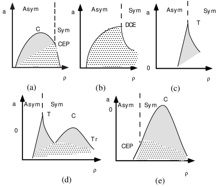
Figure 36: Schematic phase diagrams obtained from the minimization of the Landau free energy in the $(a,\rho)$ plane, corresponding to the five types discussed in the text. The transition from symmetric to asymmetric sponge can be either continuous (dashed line) or first order (solid line). T is a tricritical point, Tr a triple point, CEP a critical endpoint, DCE a double critical endpoint, and C a liquid-gas type critical point. From D. Roux, C. Coulon, M. E. Cates, J. Phys. Chem. 96 4174 (1992).

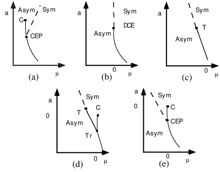
Figure 37: Phase diagrams (as above) in the $(a,\mu)$ plane. From D. Roux, C. Coulon, M. E. Cates, J. Phys. Chem. 96 4174 (1992).

• When $\rho^{*}>0,$ there is a critical line (CL) for large values of $a$ ($a>a^{*}_{1}=1/2-{\rho^{*}}^{2}$), separating the symmetric phase ($\eta_{\rm m}(\rho)=0$) from the asymmetric one. This line ends in a critical endpoint (CEP) where the CL meets a first-order line. This first-order line end at a critical point (CP) at $\rho=0,$ $a=1/2,$ which corresponds to a demixtion critical point between two asymmetric sponge phases, with different amphiphile concentration. For $a<a^{*}_{1},$ the first order line separates a symmetric from an asymmetric phase.

• When $\rho^{*}=0,$ the line of continuous transition separating the symmetric from the asymmetric phase ends at a double critical endpoint (DCE) at $\rho=0,$ $a=a_{\rm c}=1/2.$ There the shape of the coexistence curve goes as $a_{\rm c}-a\propto(\rho-\rho^{*})^{2}$ on one side to $\propto(\rho-\rho^{*})^{1/2}$ on the other side. There is no longer a separate ordinary critical point.

• When $-1/4<\rho^{*}<0,$ the symmetric and asymmetric phase are separated by a second order line for $a>a^{*}_{2}=1/2-3{\rho^{*}}^{2},$ and by a first order line for $a<a^{*}_{2}.$ These lines meet at a tricritical point.

• For $-1/2<\rho^{*}<-1/4,$ one also finds a first order line between two symmetric phases. This line ends at a critical point at $a=0,$ $\rho=0.$

• When $\rho^{*}<-1/2,$ the tricritical point T disappears and the continuous transition between symmetric and asymmetric phase ends at a critical endpoint (CEP).

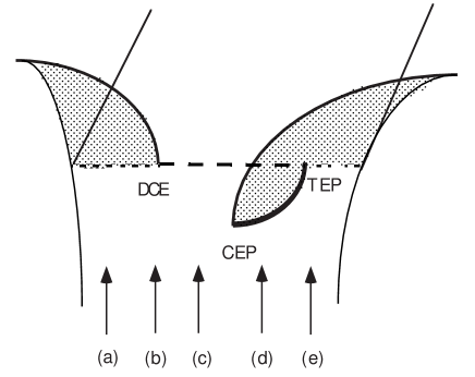
Figure 38: Representation of the Landau phase diagram in the $(a,\mu,A)$ space. Continuous line: line of critical points. Broken line: line of tricritical points. Thick line: line of triple points. Dotted line: line of critical endpoints. DCE: double critical endpoint; CE: critical endpoint; TCE: tricritical endpoint. From D. Roux, C. Coulon, M. E. Cates, J. Phys. Chem. 96 4174 (1992).

Upon looking at this phase diagram it is possible to identify the starting point of the expansion as the double critical endpoint (DCE) appearing in the diagram of Type (b). This high order critical point has in fact an “upper critical dimension” of 8/3. Therefore, the mean field treatment describes correctly the behavior around this point for three dimensional systems. On the other hand, the corrections to mean-field theory are very weak (logarithmic) around the tricritical point. One should thus expect the mean field predictions to be satisfied in a wide region for systems which happen to be near the DCE or the tricritical point T.

The occurrence of a line of tricritical points in the $(a,A,\rho)$ plane implies that, even in a binary surfactant-solvent system there is a finite probability of finding a tricritical point in a $(\phi,T)$ phase diagram, without any special adjustment of other thermodynamic variables.

Since the Landau expansion obtained above has two independent parameters (up to rescalings), and since the elastic description of bilayers has two independent elastic coefficients $\kappa$ and $\overline{\kappa},$ it should be possible to span the whole of the phase diagram by varying $\kappa$ and $\overline{\kappa}.$ In practice one can vary these quantities by adjusting concentrations of cosurfactants, salt, etc. These systems may therefore provide a testing ground for theories of higher order critical behavior.

In order to investigate the behavior of correlation function, one adds suitable gradient terms to the expansion (6.16). They involve the gradients of the two order parameters $\rho$ and $\eta,$ although only the $\rho$-$\rho$ correlations are directly observable. The most general form of the gradient terms is

$$\Delta\Phi=\frac{\gamma_{\rho}}{2}|\vec{\nabla}\rho|^{2}+\frac{\gamma_{\eta}}{2}|\vec{\nabla}\eta|^{2}+\frac{\gamma_{\rm c}}{2}\eta|\vec{\nabla}\eta\cdot\vec{\nabla}\rho|.$$ (6.21)

In the simple case in which $\gamma_{\rho}=\gamma_{\rm c}=0,$ it is possible to calculate exactly the correlations within the Gaussian approach [104]. The third term in eq. (6.21) is not quadratic in the fluctuating fields and prevents the use of the Gaussian approach when $\gamma_{\rm c}\neq 0.$ In this case, the probability distribution for $\rho(\vec{r})$ depends only on the local value of $\eta(\vec{r}).$ One can then integrate over the $\rho(\vec{r})$ field, obtaining an effective potential for the $\eta$ field:

$$\Gamma[\eta]=\int{\rm d}\vec{r}\,\left\{\frac{A^{\prime}}{2}\eta^{2}+\frac{\lambda}{4}\eta^{4}+\frac{\gamma_{\eta}}{2}|\vec{\nabla}\eta|^{2}\right\},$$ (6.22)

where $A^{\prime}=A+\mu/a,$ and $\lambda=1-a/2.$ This form implies

$$\left<\eta(\vec{r})\eta(0)\right>=\frac{\mathop{\rm e}\nolimits^{-r/\xi_{\eta}}}{4\pi\gamma_{\eta}r},$$ (6.23)

where $\xi_{\eta}=\gamma_{\eta}/A^{\prime}.$

The amphiphile concentration-concentration correlation function is defined by

$$g(\vec{r})=\left<\delta\rho(\vec{r})\delta\rho(0)\right>,$$ (6.24)

where $\delta\rho(\vec{r})=\rho(\vec{r})-\left<\rho\right>.$ It contains two contributions: the direct contribution, which in our hypotheses is very short-ranged (delta-like), and an indirect contribution, due to its coupling to the $\eta$ fluctuations. It is not difficult to see that one has in fact

$$g(\vec{r})=\frac{1}{a}\delta(\vec{r})+\frac{1}{4a^{2}}\left[\left<\eta^{2}(\vec{r})\eta^{2}(0)\right>^{2}-\left<\eta^{2}\right>^{2}\right].$$ (6.25)

Since we assume gaussian fluctuations, we have

$$\left<\eta^{2}(\vec{r})\eta^{2}(0)\right>=\left<\eta^{2}\right>^{2}+2\left<\eta(\vec{r})\eta(0)\right>^{2}.$$ (6.26)

By using the expression of the correlations of $\eta$ obtained above, we have

$$g(\vec{r})=\frac{\delta(\vec{r})}{a}+\frac{1}{4a^{2}}\frac{\mathop{\rm e}\nolimits^{-2r/\xi_{\eta}}}{(4\pi\gamma_{\eta}r)^{2}},$$ (6.27)

whose Fourier transform is

$$I(q)=C_{1}\left[C_{2}+\frac{\tan^{-1}(q\xi_{\eta}/2)}{q\xi_{\eta}/2}\right],$$ (6.28)

where

$$C_{1}=\frac{\xi_{\eta}}{16\pi a^{2}\gamma_{\eta}^{2}};\qquad C_{2}=\frac{16\pi a\gamma_{\eta}^{2}}{\xi_{\eta}}.$$ (6.29)

This expression can be compared with the results of light scattering experiments. It involves a $1/q+{\rm const.}$ behavior at large $q$ instead of the more usual (Ornstein-Zernike) one: $1/q^{2}+{\rm const.}$ The result should hold when the hypothesis of neglecting $\gamma_{\rho}$ and $\gamma_{\rm c}$ applies: i.e., near the critical symmetric-asymmetric line and away from the tricritical point.

A perturbation method [105, App. A] can be introduced to obtain the expression for $I(q)$ in the general case. The result reads

$$I(q)=\left<|\delta\rho_{q}^{2}|\right>=\frac{1}{a+\gamma_{\rho}q^{2}}+K\frac{\left(1+(\gamma_{\rm c}q^{2}/2)\right)^{2}}{(a+\gamma_{\rho}q^{2})^{2}}\frac{\tan^{-1}(q\xi_{\eta}/2)}{q\xi_{\eta}/2},$$ (6.30)

for the symmetric sponge phase, and

$$I(q) = \left<|\delta\rho_{q}^{2}|\right>=\frac{1}{a+\gamma_{\rho}q^{2}}$$ (6.31)

$$+\frac{\left(1+(\gamma_{\rm c}q^{2}/2)\right)^{2}}{(a+\gamma_{\rho}q^{2})^{2}}\left[\frac{K_{1}\left<\eta\right>^{2}}{A+\gamma_{\rho}q^{2}}+K_{2}\frac{\tan^{-1}(q\xi_{\eta}/2)}{q\xi_{\eta}/2}\right],$$

for the asymmetric sponge phase.

Two different experimental situations have been analyzed by light scattering. In the first case [104], one has studied an oil-rich sponge phase as a function of membrane concentration (this experiment will be denoted as “oil” dilution). In the system under investigation, the sponge phase undergoes a first-order transition to a phase of practically pure solvent. In the second case [24, 25], one has studied a water-rich system which exhibits a second-order phase transition between a symmetric and an asymmetric sponge phase. The transition is made apparent by a maximum turbidity line (MTL) separating the two isotropic phases. This is the line where the structure factor $I(q)$ (proportional to the osmotic compressibility) diverges at $q=0,$ corresponding to very large fluctuations in the amphiphile concentration. In this way the rather remarkable feat of exhibiting a symmetry breaking which cannot be directly observed has been achieved. This experiment will be denoted as “water” dilution. More recently, there have been careful experiments on the quaternary system Ma-octylbenzenesulfonate (OBS)/$n$-pentanol/brine [40]. These experiments challenge the picture of the asymmetric-symmetric transition given above, and will be discussed later.

The inverse scattering intensity $1/I(q)$ measured in oil dilution experiments is shown in fig. 39 as a function of the wavenumber $q.$ The form is strikingly different from the Ornstein-Zernike (dotted line), and fits well to the simple form (6.28) (solid lines). The fact that the simple expression works so well indicates that the correlation length for $\rho$ is rather small. It is possible to extract from the data the ratio of the arctan to the constant term appearing in eq. (6.28). This ratio turns out to be about 2/3, and is a measure of the relative importance of the fluctuations of $\eta$ with respect to the fluctuations of amphiphile concentration.

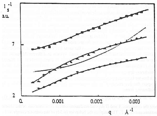
Figure 39: Plot of the inverse scattering intensity against $q$ for a sponge phase at different concentrations. Dotted line: Ornstein-Zernike form. Solid lines: eq. (133). From D. Roux, C. Coulon, M. E. Cates, J. Phys. Chem. 96 4174 (1992).

The osmotic compressibility $I(0)$ as a function of the amphiphile volume fraction $\phi$ varies approximately as $1/\phi,$ but with logarithmic corrections:

$$I(0)\propto\left(\phi\log(\phi/\phi^{*})\right).$$ (6.32)

This behavior can be understood in terms of the scaling laws [65, 101] of the free energy, which derive from the scale invariance of the Helfrich hamiltonian and the renormalization of the elastic constants. As we have seen, if all lengths are dilated by a factor $\lambda,$ the Helfrich hamiltonian remains invariant. In this transformation, the volume ratio $\phi$ remains invariant, although the surface area per unit volume is decreased by a factor $\lambda^{-1}.$ However, the membrane thickness $\delta$ is also scaled by $\lambda.$ Microstates of the original and of the rescaled system have the same energy, and therefore the two systems should possess the same free energy. In order to use this argument to describe the behavior of the same system at different dilutions, we observe that the dilated system (with volume ratio $\phi$) corresponds to the diluted system (with volume ratio $\phi/\lambda$) except that its thickness $\delta$ has been rescaled. Now the thickness appears as a cutoff in the renormalization of the elastic constants, which has we have seen produce logarithmic terms in the free energy. As a result, we expect the free energy $F$ of the solution to depend on the volume ratio $\phi$ in the following form:

$$F=k_{\rm B}T\phi^{3}(A+B\log\phi),$$ (6.33)

where the constants $A$ and $B$ depend on dimensionless combinations of the elastic constants and of $k_{\rm B}T.$ This implies the behavior (6.32) of the osmotic compressibility. The logarithmic corrections observed in $I(0)$ are therefore an experimental evidence for the renormalization of the elastic constants.

The water dilution experiments allow to exhibit the divergence of the correlation length $\xi_{\eta}$ and of the osmotic compressibility $I(0)$ at the symmetric-asymmetric transition. Experimentally in particular $I(0)\propto(\mu-\mu_{\rm c})^{-\zeta},$ where $\zeta\simeq 0.5.$ The Landau-Ginzburg approach predicts $I(0)\propto(\mu-\mu_{\rm c})^{-1/2}.$ However, the relation between density and chemical potential is singular at the transition, and the exponents undergo the so-called Fisher renormalization [41]. One has $I(0)\propto(\rho-\rho_{\rm c})^{-1}$ near the tricritical point. Near the critical point one should use nonclassical (Ising) exponents, and the Fisher renormalization has only a small effect. The result reads $I(0)\propto(\rho-\rho_{\rm c})^{-\alpha/(1-\alpha)},$ where $\alpha\simeq 0.11$ is the specific heat exponent. This yields $\zeta\simeq 0.12,$ also in contrast with the measured value. This discrepancy may arise from a crossover from critical to tricritcal behavior, but has not yet been solved.

Lamellar phases

Membranes can assume two forms that minimize the bending energy: as a stack of planar sheets, or as periodic structures of minimal surfaces (plumber’s nightmare). In both cases the mean curvature vanishes, and therefore the free energy of the structure is determined by the contribution of the gaussian rigidity and by fluctuation effects. Lamellar phases have been observed for a long time, and they are usually known as L_α phases [84].

The stability of the lamellar phases arises from a compromise between the area coefficient $\tau_{0},$ which wants to pack the layers as close as possible, and the interaction between the lamellae. The interaction between neutral membranes (for the electrostatic properties of membranes I refer to the review by D. Andelman [1]) arises from the following sources:

• A strong, short range repulsion due to the hydration interaction, yielding the interaction potential per unit area (as a function of the membrane spacing $d$) $V_{\rm h}(d)=A_{\rm h}\exp(-d/\lambda_{\rm h}).$

• A long range attraction due to the van der Waals forces:

  $$V_{\rm VW}(d) = -\frac{W}{12\pi}\left[\frac{1}{d^{2}}-\frac{2}{(d+\delta)^{2}}+\frac{1}{(d+2\delta)^{2}}\right],$$ (6.34)

  $$\sim -\frac{W}{2\pi}\frac{\delta^{2}}{d^{4}},\qquad\hbox{for }d\gg\delta.$$

  Here $\delta$ is the bilayer thickness and the parameter $W$ is known as the Hamaker constant.

• The long range steric repulsion, due to the occasional collision between lamellae [56]:

  $$V_{\rm st}(d)=c_{\rm H}\frac{(k_{\rm B}T)^{2}}{\kappa(d-\delta)^{2}}.$$ (6.35)

  Here $c_{\rm H}$ is a universal coefficient, over whose value there is some controversy [56, 49, 29].

However, one cannot simply sum up these contributions to obtain an effective potential $V_{\rm eff}(d).$ This potential has a minimum either at very short distances or at infinite separation: as a consequence one would have a first order transition between lamellar phases at high amphiphile concentration and a practically pure solvent. On the other hand very dilute lamellar phases (where $d$ can be as large as 1 m$\mu$) have been observed [76].

Lipowsky and Leibler [81] introducend a complicated functional renormalization scheme to attack the problem, and obtained a continuous transition between a state of “bound” lamellae and one of “unbound” lamellae, as the Hamaker constant $W$ crossed a critical value $W_{\rm c}.$ In this theory, the mean lamellar spacing $\bar{d}$ diverges like a power law near the transition: $\bar{d}\sim(W-W_{\rm c})^{-\psi},$ where $\psi=1.00\pm 0.03.$ This result did not appear to admit a simpler description.

Recently, Milner and Roux [88] as well as Helfrich [60] have proposed simpler (Flory-like) explanations of this continuous “unbinding” transition. However, the theory of Milner and Roux applies to the uniform lamellar phase, whereas the one by Helfrich describes the unbinding of a finite stack of $n$ layers from a wall. We shall thus dwell on the theory by Milner and Roux. First of all, one chooses the volume ratio $\phi$ of the amphiphile as the order parameter. Then the free energy is obtained in analogy with the van der Waals theory of the liquid-gas transition, by adding to the Helfrich estimate of the entropy of the stack (which only takes into account the hard-wall repulsion) a term representing the correction to the second virial coefficient due to the other interactions. In analogy with the Flory-Huggins theory of polymers, the entropy term is estimated in the absence of all correlations due to the attractive interactions, and in the correction to the virial coefficient one neglects the connectivity of the surface. This enthalpic correction is referred to “patches” of the membrane of size $\nu=\ell_{0}^{2}\delta,$ where $\ell_{0}^{2}=(\kappa/k_{\rm B}T)\delta^{2}$ is the shortest length where the membrane could bend. The result reads

$$f_{\rm lam}(\phi)=\frac{c_{\rm H}(k_{\rm B}T)^{2}}{\kappa\delta^{3}}\phi^{3}-k_{\rm B}T\chi\phi^{2}.$$ (6.36)

The coefficient $\chi$ appearing in the enthalpic correction can be given as a function of the interaction $U_{\nu}(\vec{r})$ between patches by

$$\chi=-\frac{1}{2\nu^{2}}\int{\rm d}^{3}\vec{r}\,\left\{1-\exp\left[-U_{\nu}(\vec{r})/k_{\rm B}T\right]\right\},$$ (6.37)

as long as the interaction between patches is sufficiently weak. We expect that $\chi$ vanishes linearly as the Hamaker constant reaches some critical value. The phase diagram can be obtained by minimizing with respect to $\phi$ the free energy

$$g(\chi,\mu)=f_{\rm lam}(\phi)-\mu\phi,$$ (6.38)

where $\mu$ is the chemical potential of the amphiphile. The resulting phase diagram is shown in fig. 40.

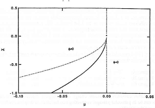
Figure 40: Phase diagram of a lamellar phase in the $(\mu,\chi)$ plane. Broken line: first order transition. Solid line: second order transition. Thin lines: spinodals. From S. T. Milner, D. Roux, J. Phys. I France 2 1741 (1992).

The expression (6.36) has the form of a Landau expansion around $\phi=0.$ In this expression, the cubic term in $\phi$ does not necessarily lead to a first order phase transition, because negative values of $\phi$ are unphysical (a similar situation arises in the mean field treatment of percolation). Therefore the order parameter vanishes at the second order transition with an exponent 1 instead of the usual mean field exponent 1/2.

Topological instabilities

We have thus found that it is possible to stabilize lamellar phases with arbitrarily small amphiphile concentrations, at least if the Hamaker constant is large enough. However, we have argued before that as the solution is diluted one should go over to isotropic or cubic phases. In order to understand this transition it is necessary to include topology changes and renormalization effects, which are absent from the previous considerations. Two recent papers deal with this problem [48, 89]. The essential point is that, while the bending rigidity $\kappa$ decreases as one goes to longer and longer length scales, the gaussian rigidity $\overline{\kappa}$ increases. Therefore structures of higher and higher genus are favoured at longer and longer scales.

In ref. [89] one starts from the expression of the Helfrich hamiltonian in terms of the principal curvatures $c_{1}$ and $c_{2}$:

$$F=\int{\rm d}A\left[\frac{1}{2}\kappa\left(c_{1}+c_{2}\right)^{2}+\overline{\kappa}\,c_{1}c_{2}\right],$$ (6.39)

and rewrites it introducing the topological rigidities $\kappa_{+}=\kappa+\overline{\kappa}/2,$ $\kappa_{-}=-\overline{\kappa}/2$:

$$F=\int{\rm d}A\left[\frac{1}{2}\kappa_{+}\left(c_{1}+c_{2}\right)^{2}+\frac{1}{2}\kappa_{-}\left(c_{1}-c_{2}\right)^{2}\right].$$ (6.40)

One has of course $\kappa=\kappa_{+}+\kappa_{-}$. When either topological rigidity vanishes, the simply connected membrane becomes unstable with respect to fluctuations leading to a different topology:

For $\kappa_{+}<0,$	towards the formation of many spherical surfaces;
for $\kappa_{-}<0,$	towards the formation of an infinite minimal surface.

Since $\kappa=\kappa_{+}+\kappa_{-},$ this instability occurs before the instability towards a continuous deformation of the membrane, which occurs when $\kappa$ becomes negative, except in the special case in which $\kappa_{+}\simeq\kappa_{-}\simeq 0.$

The topological rigidities renormalize with respect to the scale $\ell$ according to the equation

$$\kappa_{\pm}(\ell)=\kappa_{\pm}-\frac{\alpha_{\pm}k_{\rm B}T}{4\pi}\log\left(\frac{\ell}{\ell_{0}}\right).$$ (6.41)

In this equation, $\ell_{0}$ is a microscopic distance (of the order of the lateral size of an amphiphilic molecule), $\kappa_{\pm}$ are the bare values of the topological rigidites, and the coefficients $\alpha_{+}=4/3,$ $\alpha_{-}=5/3$ can be expressed in terms of the renormalization coefficients $\alpha_{\kappa}=-3,$ $\alpha_{\overline{\kappa}}=10/3$ for $\kappa$ and $\overline{\kappa}.$ This renormalization group equation defines two characteristic lengths $\xi_{\pm}\propto\exp\left(4\pi\kappa_{\pm}/(\alpha_{\pm}k_{\rm B}T)\right)$ for the onset of the topological instabilities. One expects that a lamellar phase will melt when the lamellar distance (or, better, the repeat distance $d=\delta/\phi$) becomes of the order of the smaller of these lengths.

In ref. [48] a more detailed physical picture of this transition is contained. One can distinguish three regimes [48]:

Regime A:	$-\overline{\kappa}<\frac{10}{9}\kappa,$	i.e.,	$\xi_{\overline{\kappa}}\ll\xi_{\kappa};$
Regime B:	$-\overline{\kappa}>\frac{10}{9}\kappa,$ but $|\overline{\kappa}+\frac{10}{9}\kappa|>O(1)\,k_{\rm B}T,$	i.e.,	$\xi_{\kappa}\ll\xi_{\overline{\kappa}};$
Regime C:	$|\overline{\kappa}+\frac{10}{9}|\kappa<O(1)\,k_{\rm B}T,$	i.e.,	$\xi_{\kappa}\sim\xi_{\overline{\kappa}}.$

The author considers the elastic energy of topological defects. These defects can be in particular passages connecting two lamellae, or droplets confined between the lamellae.

Let us first consider a passage connecting two lamellae a distance $d$ apart. Its curvature energy can be estimated as

$$E_{\rm p}=O(1)\,\kappa(\ell)\left(\frac{r}{\ell}\right)^{2}-4\pi\overline{\kappa}(r),$$ (6.42)

where $r$ is the size of the passage neck, and $\ell$ is the lateral size of the passage deformation region. At distances from the neck smaller than $\ell,$ the presence of the passage curves the membrane giving rise to the first term in eq. (6.42). The second term in this equation is the gaussian curvature contribution, and originates essentially from the region of the neck. Therefore the two rigidities are evaluated at different scales. (This effect is not taken into account in ref. [89]). The passage deformation region is approximately a catenoid, yielding the condition $d\simeq 2r\log(\ell/r),$ relating $r$ and $\ell.$ We let this constraint in eq. (6.42) and obtain the equilibrium energy and size of the passage, as a function of $d.$ Assuming $\kappa(d)\gg k_{\rm B}T,$ and neglecting slowly varying logarithmic factors, we obtain

$$E_{\rm p} = -\alpha_{\overline{\kappa}}k_{\rm B}T\log\frac{d}{\xi_{\overline{\kappa}}},$$ (6.43)

$$\ell_{\rm eq} = O(1)\left(\frac{\kappa(d)}{k_{\rm B}T}\right)^{1/2}d,$$ (6.44)

$$r_{\rm eq} = O(1)d.$$ (6.45)

The elastic energy of the passage decreases as $d$ increases, and becomes negative as $d$ becomes of order $\xi_{\overline{\kappa}}.$ On the other hand, the deformation region $\ell_{\rm eq}$ increases with $d.$

The interaction among passages can be represented by a hard core repulsion, with effective hard core size $\ell_{\rm eq}.$ When the area density of $n_{\rm p}$ of passages is smaller than $\ell_{\rm eq}^{-2},$ a simple grand canonical calculation yields $n_{\rm p}(d)\simeq n_{0}(d),$ with

$$n_{0}(d)=\left(\frac{\kappa(d)}{k_{\rm B}T}\right)^{2}\frac{1}{d^{2}}\left(\frac{d}{\xi_{\overline{\kappa}}}\right)^{\alpha_{\overline{\kappa}}}\propto d^{\alpha_{\overline{\kappa}}-2}=d^{4/3},$$ (6.46)

which increases with increasing $d.$ Such a growth of the passage density was observed by Harbich et al. in egg-lecithin membrane stacks [54]. The free energy of the “passage fluid” per unit membrane area is given by $F_{\rm p}(d)=-k_{\rm B}Tn_{0}(d)\sim-d^{4/3}.$ The passages begin to overlap when $d$ becomes of order $d^{*},$ where

$$d^{*}=\left(\frac{k_{\rm B}T}{\kappa(\xi_{\overline{\kappa}})}\right)^{3/\alpha_{\overline{\kappa}}}\xi_{\overline{\kappa}}\sim\xi_{\overline{\kappa}}.$$ (6.47)

In this situation, the free energy can be estimated by minimizing with respect to the passage density $n$ a trial free energy containing the contribution of the hard core repulsion:

$$F_{\rm p}(n,d)=k_{\rm B}Tn\log\left(\frac{n}{\mathop{\rm e}\nolimits n_{0}(d)}\right)-k_{\rm B}Tn\log\left(1-n\ell_{\rm eq}^{2}\right).$$ (6.48)

The first term reproduces the dilute result $n=n_{0}(d),$ while the second represents the free energy increase due to the hard-core repulsion. We obtain therefore $n_{\rm p}\simeq\ell_{\rm eq}^{-2}$ for $d\gg d^{*},$ with a free energy

$$F_{\rm p}(d) \simeq -O(1)\left(\frac{k_{\rm B}T}{\ell_{\rm eq}^{2}}\right)\log\left(n_{0}(d)\ell_{\rm eq}^{2}\right)$$ (6.49)

$$\simeq -O(1)\frac{(k_{\rm B}T)^{2}}{\kappa(d)d^{2}}\log\left(1+(d/d^{*})^{\alpha_{\overline{\kappa}}}\right).$$

This free energy corresponds to an attractive interaction between membrane pairs, which tends to keep them at a distance $d\sim\xi_{\overline{\kappa}}.$ This attraction actually dominates over the Helfrich steric repulsion

$$V_{\rm st}(d)=-c_{\rm H}\frac{(k_{\rm B}T)^{2}}{d^{2}}.$$ (6.50)

for $d>\xi_{\overline{\kappa}}.$

The free energy of the lamellar phase per unit volume is given by

$$F_{\rm lam}(\tau_{0})=\min_{d}\Phi(d,\tau_{0}),$$ (6.51)

where $\tau_{0}$ is the area coefficient (proportional to the chemical potential of surfactant) and

$$\Phi(d,\tau_{0})=\frac{1}{d}\left[\tau_{0}+F_{\rm p}(d)+V_{\rm st}(d)\right].$$ (6.52)

This expression does not include the van der Waals interaction. In the absence of the passage term, one has a single minimum for $\tau_{0}<0,$ at $d=d_{\rm eq}\sim|\tau_{0}|^{-1/2}.$ One would thus expect a swelling of the lamellar phase until $d\sim\xi_{\kappa},$ where the lamellae crumple. But the inclusion of the passage interaction changes the behavior, and $d_{\rm eq}$ remains essentially fixed at $\xi_{\overline{\kappa}}$ also for positive $\tau_{0},$ where one would expect a diluted droplet phase. The free energy of the droplet phase can be shown to be essentially zero compared to that of eq. (6.51). The lamellar phase therefore gives way to the droplet phase when the free energy (6.51) vanishes, what happens for $\tau_{0}\sim(k_{\rm B}T)^{2}/(\kappa(\xi_{\overline{\kappa}})\xi_{\overline{\kappa}})^{2}.$ This only holds in regime A, where $\xi_{\overline{\kappa}}\ll\xi_{\kappa}.$ In regime A one therefore expects the lamellar phase (with a repeat distance $d\sim d^{*}$) to remain stable also for a positive area coefficient. One would thus have a strong first-order phase transition between a passage-rich, but still orientationally ordered, lamellar phase and a dilute droplet phase.

In regime B, on the other hand, passages will be very dilute and the most important role is played by the droplets. The length scale of droplets is fixed by $\xi_{+},$ which is much smaller than $\xi_{\kappa}$ in this regime. In ref. [48] it is assumed that the elastic energy of a droplet of scale $R$ is given by $E_{\rm d}(R)=8\pi\kappa_{+}(R)=2\alpha_{+}k_{\rm B}T\log(\xi_{+}/R).$ (The results would probably have to be modified in view of the results of ref. [90].) By means of this expression, it is possible to compute the free energy, per unit area of lamella, of a polydisperse solution of droplets confined between two lamellae. The result reads

$$F_{\rm d}(d)=d\,{\cal F}_{\rm d}+f_{\rm d}(d),$$ (6.53)

where ${\cal F}_{\rm d}$ is the free energy per unit volume of the droplet phase, which in our hypotheses is given by

$${\cal F}_{\rm d}=-O(1)\frac{\kappa^{2}}{k_{\rm B}T}\left(\frac{\ell_{0}}{\xi_{+}}\right)^{2\alpha_{+}}\ell_{0}^{-3}.$$ (6.54)

The effects of the confinement are contained in $f_{\rm d}(d),$ which is given by

$$f_{\rm d}(d)=O(1)\frac{(\kappa(d))}{k_{\rm B}T}\left(\frac{d}{\xi_{+}}\right)^{2\alpha_{+}}d^{-2}\sim d^{2/3},$$ (6.55)

corresponding to an attractive interaction between the lamellae. Therefore the difference between the free energy density of the lamellar and the droplet phase exhibits a minimum at a value $d^{*}=d^{*}(\tau_{0}).$ For a critical value $\tau_{\rm c}\sim-(k_{\rm B}T)^{2}/(\kappa(d_{\rm max})d_{\rm max}^{2})$ of $\tau_{0}$ the free energy difference vanishes and the lamellar phase melts into the droplet phase. The maximal distance $d_{\rm max}$ between the lamellae is given by

$$d_{\rm max}=d^{*}(\tau_{\rm c})\sim\left(\frac{k_{\rm B}T}{\kappa(\xi_{\rm d})}\right)^{3/\alpha_{+}}\xi_{\rm d}\sim\xi_{\rm d}.$$ (6.56)

This is also the radius $R_{\rm max}$ of the largest droplets.

In this regime it should therefore be possible to observe a weak first-order transition to a dense droplet phase. This transition takes place when $d$ reaches the value $\xi_{+}.$ A transition to an isotropic sponge phase can only occur in regime C (corresponding to $d_{\rm max}\sim R_{\rm max}\sim\xi_{\overline{\kappa}}\sim\xi_{\kappa}\sim\xi_{+}$) where the creation of passages between the largest droplets is favored.

These expectations agree with those of ref. [89] in regime B and regime C. The predictions for regime A are different. In particular they contradict the prediction made in ref. [89] of a transition from the lamellar phase into a L₃ phase of multiply-connected surfaces with small mean curvature.

Free edges and gauge theories

I discuss in this subsection the elegant connection made by Huse andLeibler [66] between the sponge phases of membranes and the $Z_{2}$ gauge-Higgs models on a lattice.

When one considers real membranes, one should also take into account the possibility of free edges. Free edges (see fig. 31(a)) involve a region with strong curvature in the amphiphilic arrangement, and where contact between water and the tails of the amphiphile is eased. It is likely therefore that these defects cost a relatively high price in terms of energy per unit length. However, this price is not infinite, and it is interesting to ask how the phase diagram of the membranes is affected by introducing them.

One can stard by adding to the Helfrich hamiltonian a term

$$F_{1}=\lambda_{0}\int{\rm d}\ell,$$ (6.57)

where the integral is over all edges, and $\lambda_{0}$ is the chemical potential per unit length, of the edges “living” on the membrane. For infinite $\lambda_{0}$ edges are suppressed and the previous results hold. When $\lambda_{0}$ is finite, we start running into difficulties in separating without ambiguities “inside” (I) from “outside” (O) in the sponge and droplet phases. Moreover, it is no more possible to define an effective surface tension, as we had done in the gedankenexperiment mentioned in the discussion of the asymmetric sponge phase. Indeed, if we try to force a macroscopic interface between a prevalently “up” and a prevalently “down” spin phase, the system will prefer to introduce a macroscopic hole in the membrane, and the free energy will be higher by a term of order $L$ (instead of order $L^{2}$) with respect to a homogeneous system.

Instead, one may consider the effects of forcing a macroscopic edge through the system. Imagine to introduce an edge along a curved line ${\cal C}_{1}$ connecting points B and C, set a distance $\ell$ apart, as in fig. 41. The length of the curved line is equal to $L.$ The system must choose the return path ${\cal C}_{2}$ connecting C to B. If the free energy cost needed to create a macroscopic patch of the membrane is small, nothing prevents the system from choosing the straight line BC as ${\cal C}_{2}$ (fig. 41(a)).

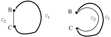
Figure 41: Theoretical construction for the definition of the macroscopic line tension. An edge (thick line) is forced in the sample, connecting points B and C along the curve ${\cal C}_{1}.$ The return path ${\cal C}_{2}$ may either be a straight line (a) or a curved line close to ${\cal C}_{1},$ depending on the energy cost of the creation of membrane patches. From D. H. Huse and S. Leibler, Phys. Rev. Lett. 66 437 (1991).

In this case, the free energy price of the free edge BC is proportional to $\ell,$ and the macroscopic line tension is nonzero. On the other hand, if the free energy cost of the membrane is large, the system prefers to return along the curve ${\cal C}_{2}$ situated very close to ${\cal C}_{1}$ (fig. 41(b)), in order to avoid creating extra surface. In this regime, the macroscopic line tension is formally zero. The first regime is expected to hold in the symmetric sponge phase. We expect the macroscopic line tension to vanish in the asymmetric sponge phase and also in the phase corresponding to the droplet phase, but in which small membrane patches with free edges are also allowed. This is the droplet-and-disc phase.

In order to understand more closely the phase diagram, let us fix the value of the microscopic line tension $\lambda_{0},$ of the rigidity $\kappa_{0},$ and let us start from a large value of the area coefficient $\tau_{0}.$ We shall be in the droplet-and-disc phase, and the edges appear as closed rings, spanned by the membrane. As $\tau_{0}$ decreases, an infinite piece of connected surface appears, although (with sufficiently large $\lambda_{0}$) the size of the edge loops remain finite: this is the asymmetric sponge regime. If we now reduce $\lambda_{0},$ one reaches a regime in which connected edge paths of infinite length are present: this is the sponge-with-free edges regime. One can picture this regime as a melt of ring polymers (the edges) of arbitrary length. These polymers are Gaussian at large lengths, and therefore have only a finite probability of coming close to themselves. However, there are an infinite number of these polymers, and different polymers will come close to each other infinitely many times. So the surface attached to one edge will almost certainly be connected to the surface attached to the other edge, and therefore one expects only one connected piece of membrane to be present.

We have therefore four different isotropic regimes: droplet-and-disc, asymmetric sponge, sponge with free edges (all three of them with a vanishing macroscopic line tension), and the symmetric sponge regime (with a nonzero line tension). Only the symmetric sponge regime is separated from the others by a bona fide phase transition.

For sufficiently large and negative $\tau_{0}$ one goes over to the orientationally ordered phases. Here, the presence of free edges is incompatible with smectic (positional) order, as we have discussed before: but we may have, or not have, a macroscopic line tension. We have therefore two nematic phases, depending on the value of the macroscopic line tension: nematic with line tension, and nematic with free edges. The resulting phase diagram in the $(\tau_{0},\lambda_{0})$ plane is sketched in fig. 42.

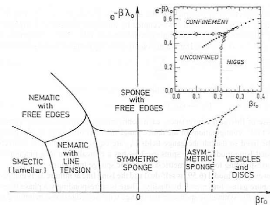
Figure 42: Schematic phase diagram for an ensemble of membranes with edges, according to D. H. Huse and S. Leibler, Phys. Rev. Lett. 66 437 (1991). The dashed lines correspond to geometric (percolation) transitions, while the solid lines show the thermodynamic phase transitions. The $\tau_{0}>0$ of the phase diagram corresponds to the phase diagram of the $Z_{2}$ gauge Higgs model shown in the inset. In the inset the dotted line is the self-duality line; the unconfined-confined transition on the vertical line has its dual equivalent in the unconfined-Higgs transition on the horizontal line.

The part of the phase diagram involving the sponge phases is in fact equivalent to the phase diagram of the $Z_{2}$ gauge-Higgs system (for a review, see, e.g., [35]). The connection can be made explicit by considering random surfaces on a lattice. The lattice length should correspond to the persistence length $\xi_{\kappa}$: at longer lengths, the bending rigidity can be neglected. Thus, let us consider a random surface living on the plaquettes of a simple cubic lattice. Label the elementary cubes by indices $i.$ One introduces Ising spins $\sigma_{i}=\pm 1$ on each elementary cube, and a gauge field $U_{ij}=\pm 1$ on each plaquette $ij$ (separating cube $i$ and cube $j$).

The plaquette $ij$ is occupied by the membrane if $\sigma_{i}U_{ij}\sigma_{j}=-1.$ The link shared by cubes $i,$ $j,$ $k,$ and $l$ is occupied by an edge (or a seam) if the number of adjacent plaquettes containing membranes is odd. This corresponds to $U_{ij}U_{jk}U_{kl}U_{li}=-1.$ The Hamiltonian corresponding to these fields is therefore

$$H=-\tau_{0}\sum_{\left<ij\right>}\sigma_{i}U_{ij}\sigma_{j}-\lambda_{0}\sum_{\left<ijkl\right>}U_{ij}U_{jk}U_{kl}U_{li}.$$ (6.58)

This hamiltonian is invariant under the gauge transformation

$$\sigma_{i}\to\epsilon_{i}\sigma_{i};\qquad U_{ij}\to\epsilon_{i}\epsilon_{j}\,U_{ij};\qquad\epsilon_{i}=\pm 1.$$ (6.59)

Because of this gauge invariance, each configuration of the membrane corresponds to $2^{N}$ configurations of the lattice gauge model. For infinite $\lambda_{0},$ the gauge may be fixed so that all the gauge fields $U_{ij}$ are equal to $+1,$ and one recovers the usual Ising model for the spins $\sigma_{i}.$ This has a critical point as a function of $\tau_{0},$ corresponding to the symmetric-asymmetric sponge transition.

However, the model (6.59) is self-dual and the Ising line at infinite $\lambda_{0}$ is mapped to the pure gauge line $\tau_{0}=0$ by duality. There is correspondingly a phase transition from the symmetric sponge to the sponge with free edges, also belonging to the Ising universality class.

Away from the $\tau_{0}=0$ or $\lambda_{0}=\infty$ lines one may exploit Monte-Carlo simulations of the $Z_{2}$ gauge system [68]. The result is that these lines of continuous transition become first-order line near the triple point where the three phases meet. A line of first-order transition also extends along the self-dual line, separating for a while the asymmetric sponge from the sponge with free edges phase, and terminating in a critical point, beyond which there is no thermodynamic singularity separating the two regimes.

As I have mentioned above, the experimental results of ref. [40] on the quaternary OBS/$n$-pentanol/brine system could not be interpreted without difficulties in the framework of the phenomenological theory of the asymmetric/symmetric transition of ref. [105]. In this system, one observes a sharp maximum of the osmotic compressibility $I(0)$ on the maximum turbidity line (MTL) far inside a one-phase region; however, the light scattering function $I(q)$ has a Ornstein-Zernike $q^{-2}$ form on the $n$-pentanol rich side of the MTL (while it deviates from this form on the $n$-pentanol poor side).

This behavior is not compatible with the predictions of ref. [105], which would imply a (weak) divergence of $I(0),$ and a different form of the scattering function, nor with the hypothesis of a tricritical behavior, because one is deep inside a one phase region (while a tricritical point is necessarily close to a two-phase region). The authors suggest to introduce a different phenomenological model, introducing a new order parameter, $m,$ linearly (and not quadratically) coupled to the amphiphile density $\rho.$ In this way one would explain both the strong divergence of $I(0)$ and the Ornstein-Zernike form of $I(q).$ The divergence is then “rounded off” because the amphiphile concentration acts as a “magnetic field” for $m,$ and the critical point is reached only for that particular value of the concentration for which the “magnetic field” vanishes.

The authors then go on to suggest that the MTL in this system can be related to the symmetric sponge/sponge-with-free-edges (S/SFE) transition considered by Huse and Leibler [66]. The idea is that the (small) alcohol molecules essentially act by reducing the line tension $\lambda_{0}$ for the formation of free edges and seams. However, I do not see how this suggestion helps in understanding the asymmetry in the form of the scattering function $I(q),$ or the apparent lack of divergence in $I(0).$ Concerning the last point the authors argue that the actual behavior of the membrane should be described by a more general model, in which edges and seams have different line tensions. However, the critical behavior of this model is still unknown.

Plumber’s nightmares

I close by a very brief discussion of plumber’s nightmare phases [65]. The free energy per unit volume of this phase as a function of the lattice constant $s$ is given by

$${\cal F}_{\rm pn}(s)\simeq C_{1}\frac{\tau_{0}}{s}+\frac{C_{2}k_{\rm B}T-C_{3}\overline{\kappa}(s)}{s^{3}}.$$ (6.60)

The density of handles is $C_{3}/(4\pi s^{3}),$ and the constants $C_{i}$ are of order unity. The lattice constant will presumably be of the order of the short-distance cutoff $\ell_{0},$ at least if the “bare” gaussian rigidity $\overline{\kappa}_{0}$ is positive. In this case, by comparing this free energy to that of the droplet phase (which is zero on the scale $\tau_{0}/\ell_{0}$) the transition to the plumber’s nightmare phase will take place when $C_{3}\overline{\kappa}_{0}\simeq C_{2}k_{\rm B}T+C_{1}\tau_{0}\ell_{0}^{2}.$ We expect the transition from the droplet phase to be strongly first-order. On the other hand one can view the transition from the lamellar side to be analogous to a “crystallization” of the passage fluid considered, e.g., in ref. [48]. In this case it should be weakly first order.

Conclusions

Unfortunately I have not been able to discuss in these notes some fascinating arguments, like the behavior of membranes with reduced symmetry (hexatic and cristalline), or made of several components. But I had presumed too much on my speed in writing and I could not abuse of the editors’ patience. I hope however that I have conveyed to you part of my fascination for this delicate field of Statistical Physics.

Appendix A Differential equations for vesicle shapes

The Euler-Lagrange equations for vesicle shapes cannot be analytically solved in general. We show in this Appendix how, limiting oneself to the consideration of axisymmetric shapes, one can transform them into a system of first-order ordinary differential equations, which can be solved numerically ([34, 96]).

The geometry is defined in fig. (43).

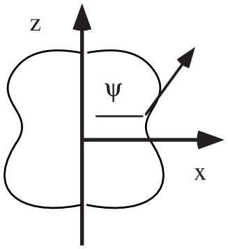
Figure 43: Axisymmetric vesicle shape: the $z$ axis is the axis of rotational symmetry.

Because of rotational symmetry, one has

$$H=c_{\rm m}+c_{\rm p},$$ (A.1)

where $c_{\rm m,p}$ are the principal curvatures (the eigenvalues of the curvature matrix $\Omega$), corresponding respectively to the meridians (m) and the parallels (p). Denoting by $\psi$ the angle between the surface normal and the $z$-axis, we have

$$c_{\rm p}=\frac{\sin\psi(x)}{x},\qquad c_{\rm m}=\cos\psi(x)\frac{{\rm d}\psi}{{\rm d}x}.$$ (A.2)

The angle $\psi(x)$ is related to the contour $z(x)$ by

$$\frac{{\rm d}z}{{\rm d}x}=-\tan\psi(x).$$ (A.3)

On the other hand, the contour $z(x)$ and the volume $V$ can be expressed in terms of $x$ and $c_{\rm p}$:

$$z(x) = z(0)-\int{\rm d}xxc_{\rm p}\left[1-(xc_{\rm p})^{2}\right]^{-\frac{1}{2}},$$ (A.4)

$${\rm d}V = \pi x^{3}c_{\rm p}\left[1-(xc_{\rm p})^{2}\right]^{-\frac{1}{2}}{\rm d}x,$$ (A.5)

$${\rm d}S = 2\pi x\left[1-(xc_{\rm p})^{2}\right]^{-\frac{1}{2}}{\rm d}x.$$ (A.6)

It is useful to replace the independent variable $x$ by the normalized surface area $s$ using the relation

$${\rm d}x=\pm\frac{2}{x}\left[1-(xc_{\rm p})^{2}\right]^{\frac{1}{2}}.$$ (A.7)

The variable $s$ ranges from $s=0$ at the upper pole to a value $s_{\rm m}$ at the dividing parallel of latitude, and then to $s=1$ at the lower pole. One has

$$\frac{{\rm d}x}{{\rm d}s}\cases{\geq 0,&for $0\leq s\leq s_{\rm m}$;\cr\leq 0,&for $s_{\rm m}\leq s\leq 1.$}$$ (A.8)

Introducing the notation $f=x^{2}$ the equations become:

$$\frac{{\rm d}c_{\rm m}}{{\rm d}s} = \pm\left(1-fc^{2}_{\rm p}\right)^{-\frac{1}{2}}\times\left\{c_{\rm p}\left[\left(c_{\rm p}-c_{0}\right)^{2}-c^{2}_{\rm m}\right]+\right.$$ (A.9)

$$+\left.\frac{2\gamma}{\kappa}c_{\rm p}+\frac{p}{\kappa}-2\left(1-fc_{\rm p}^{2}\right)\frac{c_{\rm m}-c_{\rm p}}{f}\right\};$$

$$\frac{{\rm d}c_{\rm p}}{{\rm d}s} = \pm 2\left(1-fc_{\rm p}^{2}\right)^{\frac{1}{2}}\frac{c_{\rm m}-c_{\rm p}}{f},$$ (A.10)

$$\frac{{\rm d}f}{{\rm d}s} = \pm 4\left(1-fc_{\rm p}^{2}\right)^{\frac{1}{2}}.$$ (A.11)

These equation have singularities for either $f(s)\to 0$ or $f(s)c_{\rm p}^{2}\to 1$. At the poles of the vesicles we have $f=0$, but at the same time the difference $c_{\rm m}-c_{\rm p}$ tends to zero. This yields the correct boundary condition at the poles:

$$\left.\frac{{\rm d}c_{\rm p}}{{\rm d}s}\right|_{\rm poles}=\frac{1}{3}\left.\frac{{\rm d}c_{\rm m}}{{\rm d}s}\right|_{\rm poles}.$$ (A.12)

The singularity for $f(s)c^{2}_{\rm p}\to 1$ is approached when $f(s)$ reaches an extremum, and should be removed by imposing that the factor in curly brackets in eq. (A.10) vanishes. This allows one to join the $\pm$ branches of the equations by expanding in a Taylor series around the value $s=s_{m}$ where $f(s)$ reaches the extremum.

One can then obtain the three curves $c_{\rm m}(s),$ $c_{\rm p}(s),$ $f(s),$ and the matching at those intermediate points $s_{\rm m}$ where $f(s)c^{2}_{\rm p}\to 1$ gives three nonlinear equations for the unknown boundary conditions $c_{\rm m}(s{=}0),$ $f(s{=}s_{\rm m}),$ and $c_{\rm m}(s{=}s_{\rm m}).$ A further integration yields the actual vesicle shape $z(x).$

Appendix B The Faddeev-Popov determinant

Let us consider the integral

$${\cal I}=\int{\rm d}^{2}\vec{x}\,f(\vec{x}),$$ (B.1)

where the function $f(x,y)$ is invariant upon rotations in the $(x,y)$ plane:

$$\vec{x}\to\vec{x}_{\theta}=\Omega(\theta)\cdot\vec{x},$$ (B.2)

where $\Omega(\theta)$ is a rotation matrix:

$$\Omega=\left(\begin{array}[]{cc}\cos\theta&-\sin\theta\\ \sin\theta&\cos\theta\end{array}\right).$$ (B.3)

It is then convenient to integrate the function over one line, whose images upon rotation sweep the whole two-dimensional plane. This line can be represented by an equation in $\vec{x}$:

$$\psi(\vec{x})=0.$$ (B.4)

Given any vector $\vec{x}$ there will be a value $\theta^{*}$ such that $\psi(\vec{x}_{\theta^{*}})=0.$ Using the properties of the delta function, we obtain

$$\int_{0}^{2\pi}{\rm d}\theta\delta\left(\psi(\vec{x}_{\theta})\right)=\left|\frac{\partial\psi(\vec{x}_{\theta})}{\partial\theta}\right|_{\theta^{*}}^{-1}.$$ (B.5)

Therefore

$${\cal I} = \int_{0}^{2\pi}{\rm d}\theta\int{\rm d}^{2}\vec{x}\,\delta\left(\psi(\vec{r}_{\theta})\right)\left|\frac{\partial\psi(\vec{x}_{\theta})}{\partial\theta}\right|f(\vec{r})$$ (B.6)

$$= 2\pi\int{\rm d}^{2}\vec{x}\,\delta\left(\psi(\vec{r})\right)\left|\frac{\partial\psi(\vec{x}_{\theta})}{\partial\theta}\right|_{\theta=0}f(\vec{r}).$$

The advantage of this expression is that all the quantities need only to be evaluated on (or near) the line $\psi(\vec{x})=0.$

The Faddeev-Popov determinant is the generalization of the factor introduced above to correct the effect of the integration over $\theta.$ We consider a general integral

$${\cal I}=\int{\rm d}\mu(x)\,f(x),$$ (B.7)

where the measure ${\rm d}\mu(x)$ and the function $f(x)$ are both invariant with respect to a $N$-dimensional group $G,$ whose elements $g$ can be represented via its $N$ generators $t_{\alpha}$:

$$g=\exp\left[\sum_{\alpha}\theta^{\alpha}t_{\alpha}\right].$$ (B.8)

We “fix the gauge”, introducing $N$ constraints $\psi_{\alpha}(x)=0,$ $i=1,\ldots,N.$ We then have

$${\cal I}=\int{\rm d}\mu(x)f(x)\,\prod_{\alpha=1}^{N}\delta\left(\psi_{\alpha}(x)\right)\,|\mathop{\rm Det}\nolimits(J_{\alpha\beta}(x))|\,{\rm vol}\,G,$$ (B.9)

where we have introduced the volume of the group $G,$ and

$$J_{\alpha\beta}(x)=\left.\frac{\partial\psi_{\alpha}(x)}{\partial\theta^{\beta}}\right|_{\theta=0}.$$ (B.10)

In our case, the relevant group is generated by the infinitesimal diffeomorphisms of the form

$$\underline{\sigma}\to\underline{\sigma}+\underline{\epsilon}(\underline{\sigma}).$$ (B.11)

The corresponding transformations on the $\vec{r}$ read

$$\vec{r}\to\vec{r}+\epsilon^{i}\partial_{i}\vec{r}.$$ (B.12)

Consider now a deformation $\vec{h}$ with respect to a background configuration $\vec{r}_{0}$:

$$\vec{r}(\underline{\sigma})=\vec{r}_{0}(\underline{\sigma})+\vec{h}(\underline{\sigma}).$$ (B.13)

The normal gauge is realized by imposing the constraints

$$\psi_{i}(\underline{\sigma})=\vec{h}(\underline{\sigma})\cdot\partial_{i}\vec{r}_{0}(\underline{\sigma})=0,\qquad i=1,2.$$ (B.14)

Let us compute how the constraints are affected by an infinitesimal diffeomorphism:

$$\delta\psi_{i}(\underline{\sigma}) = \delta\left(\vec{r}-\vec{r}_{0}\right)\cdot\partial_{i}\vec{r}_{0}=\delta\vec{h}\cdot\partial_{i}\vec{r}_{0}$$ (B.15)

$$= \epsilon^{j}\partial_{j}\vec{r}\cdot\partial_{i}\vec{r}_{0}$$

$$= \epsilon^{j}\left(\partial_{j}\vec{r}_{0}+\partial_{j}\vec{h}\right)\cdot\partial_{i}\vec{r}_{0}$$

$$= \epsilon^{j}\left(g_{ij}+\partial_{j}\vec{h}\cdot\partial^{i}\vec{r}_{0}\right).$$

We see that this expression is purely local. Therefore, in this gauge, the Faddeev-Popov determinant reads

$$\Delta_{\rm FP}=\prod_{\underline{\sigma}}\mathop{\rm Det}\nolimits\left[g_{ij}(\underline{\sigma})+\partial_{i}\vec{h}(\underline{\sigma})\cdot\partial_{j}\vec{r}_{0}(\underline{\sigma})\right].$$ (B.16)

In the particular case of the Monge representation, $\partial_{i}\vec{h}(\underline{\sigma})\cdot\partial_{j}\vec{r}_{0}(\underline{\sigma})=0,$ so that the Faddeev-Popov determinant is trivial.

Appendix C One-loop calculation of the renormalization group flow

In this Appendix I report the calculation of the renormalization group flow to one loop, following essentially [31, 28, 52]. We use the method of the background field. We take the reference configuration to be parametrically described by $\vec{r}_{0}(\underline{\sigma})$ and we sum over all configurations $\vec{r}(\underline{\sigma})$ such that: (i) they are sufficiently “close” to the reference one (so that the deformation $\vec{h}(\underline{\sigma})$ is small); (ii) the wavenumbers contained in the Fourer transform of $\vec{h}(\underline{\sigma})$ belong to the infinitesimal shell $\Lambda/s<|\underline{q}|<\Lambda.$ We write the effective Wilson hamiltonian ${\cal H}_{\rm eff}(s)$ as follows:

$${\cal H}_{\rm eff}(s)=-k_{\rm B}T\log\int_{s}{\cal D}\vec{h}\exp\left\{-\frac{F[\vec{r}_{0}+\vec{h}]}{k_{\rm B}T}\right\}+\int{\rm d}A\,\vec{\lambda}\cdot\vec{r}_{0},$$ (C.1)

where $\int_{s}$ is a reminder on the constraint on the fluctuation wavenumber, and $\vec{\lambda}$ is the external field needed to set $\left<\vec{r}\right>_{\lambda}=0.$ We can expand $F[\vec{r}_{0}+\vec{h}]$ in powers of $\vec{h}$ up to second order. The contribution of the first order will cancel with the second term of the rhs of eq. (C.1). We obtain

$${\cal H}_{\rm eff}(s) = F[\vec{r}_{0}]-\log\int_{s}{\cal D}\vec{h}\exp\left\{-\frac{\delta^{2}F[\vec{r}_{0}+\vec{h}]}{k_{\rm B}T}\right\}$$ (C.2)

$$= F[\vec{r}_{0}]+\frac{k_{\rm B}T}{2}\mathop{\rm Tr}\nolimits_{s}\log\left\{\frac{\delta^{2}F}{\delta h\delta h}\right\},$$

where $\delta^{2}F$ is the second variation of the Helfrich hamiltonian with respect to $\vec{h}.$

We now introduce the metric tensor $g_{ij}$ of the reference configuration $\vec{r}_{0}$:

$$g_{ij}(\underline{\sigma})=\partial_{i}\vec{r}_{0}(\underline{\sigma})\cdot\partial_{j}\vec{r}_{0}(\underline{\sigma}).$$ (C.3)

On the basis of $g_{ij}$ we can define the covariant derivative $D_{i}.$ We can then express the curvature tensor $\vec{\Omega}_{ij}$ as follows:

$$\vec{\Omega}_{ij}=D_{i}D_{j}\vec{r}_{0}.$$ (C.4)

One can check that $\Omega_{ij}$ is normal to the surface for any $i,$ $j.$ It can therefore represented by $\vec{\Omega}_{ij}=\Omega_{ij}\vec{n},$ where $\vec{n}$ is the normal unit vector. The Gaussian curvature $K$ and the square of the mean curvature $H^{2}$ are then given by

$$H^{2} = \Omega_{i}{}^{i}\Omega_{j}{}^{j};$$ (C.5)

$$2K = \Omega_{i}{}^{i}\Omega_{j}{}^{j}-\Omega_{i}{}^{j}\Omega^{i}{}_{j}.$$ (C.6)

We use the normal gauge, and represent the deformation $\vec{h}$ by the scalar $\nu,$ defined by $\vec{h}=\nu\vec{n}.$ We then have:

$$\delta^{2}F = \int{\rm d}A\,\nu\left\{\kappa\left[\Delta^{2}+\frac{1}{2}(H^{2}-4K)+2H\Omega^{ij}D_{i}D_{j}+\ldots\right]\right.$$ (C.7)

$$\left.+\tau\left[-\Delta+2K\right]\right\}\nu,$$

where we have introduced the Laplacian (with respect to the metric tensor $g_{ij}$):

$$\Delta=D_{i}D^{i}.$$ (C.8)

The gaussian curvature term drops out of the variation. We have neglected terms which are irrelevant in our approximations, being of higher order in the curvatures. When integrating upon the fluctuations, the $\mathop{\rm Tr}\nolimits_{s}\log$ term in eq. (C.2) can be replaced by $\int{\rm d}\underline{\sigma}\int_{s}{\rm d}^{2}\underline{q}(2\pi)^{-2},$ and the operator $\Delta$ by $q^{2}.$ The result reads

$${\cal H}_{\rm eff}(s) = F+\frac{k_{\rm B}T}{2}\int{\rm d}A\frac{\Lambda^{2}\epsilon}{2\pi}$$ (C.9)

$$\times\log\left\{\frac{1}{k_{\rm B}T\Lambda^{4}}\left[\kappa\Lambda^{4}+\tau\Lambda^{2}-\frac{3}{2}\kappa H^{2}\Lambda^{2}+\frac{10}{3}\kappa K\right]\right\}.$$

We can read off this formula the effective parameters:

$$\tau_{\rm eff}(s) = \tau+\epsilon\Lambda^{2}\frac{k_{\rm B}T}{4\pi}\log\left(\frac{\kappa}{k_{\rm B}T}+\frac{\tau}{k_{\rm B}T\Lambda^{2}}\right),$$ (C.10)

$$\kappa_{\rm eff}(s) = \kappa-\epsilon\frac{3k_{\rm B}T}{4\pi}\frac{1}{1+(\tau/\Lambda^{2})},$$ (C.11)

$$\overline{\kappa}_{\rm eff}(s) = \overline{\kappa}+\epsilon\frac{5k_{\rm B}T}{3\pi}\frac{1}{1+(\tau/\Lambda^{2})}.$$ (C.12)

However, this formula does not consider the contributions of the measure terms [13]. Their effect is a shift in $\tau_{\rm eff}$:

$$\tau_{\rm eff}\to\tau_{\rm eff}^{\prime}=\tau_{\rm eff}-\epsilon\frac{\Lambda^{2}}{4\pi}k_{\rm B}T\log\left(\frac{\kappa}{k_{\rm B}T}\right).$$ (C.13)

Taking into account this contribution and rescaling back the lengths we obtain the renormalized couplings, which obey the renormalization group equations

$$s\frac{\partial\tau}{\partial s} = 2\tau+\frac{\Lambda^{2}}{4\pi}k_{\rm B}T\log\left(1+\frac{\tau}{\kappa\Lambda^{2}}\right),$$ (C.14)

$$s\frac{\partial\kappa}{\partial s} = -\frac{3k_{\rm B}T}{4\pi}\frac{1}{1+(\tau/\Lambda^{2})},$$ (C.15)

$$s\frac{\partial\overline{\kappa}}{\partial s} = \frac{5k_{\rm B}T}{3\pi}\frac{1}{1+(\tau/\Lambda^{2})}.$$ (C.16)

Appendix D The Liouville model

The Liouville model is defined by the hamiltonian

$${\cal H}[\vec{r},g_{ij}]=\gamma_{0}\int{\rm d}^{2}\underline{\sigma}\sqrt{g}+\lambda\int{\rm d}^{2}\underline{\sigma}\sqrt{g}\,g^{ij}\partial_{i}\vec{r}\cdot\partial_{j}\vec{r}.$$ (D.1)

The metric tensor $g_{ij}$ fluctuates in this model, and is not induced by the membrane configuration described by $\vec{r}.$

The Liouville model is best studied in the conformal gauge where the internal metric tensor $g_{ij}$ takes the form

$$g_{ij}=\mathop{\rm e}\nolimits^{\phi}\delta_{ij}.$$ (D.2)

It is always possible to construct locally such a coordinate system (see, e.g., [28, Sec. 2.8]). In this system, the gaussian curvature reads

$$K(\underline{\sigma})=-\frac{1}{2}\mathop{\rm e}\nolimits^{-\phi(\underline{\sigma})}\left(\frac{\partial^{2}}{\partial\sigma_{1}^{2}}+\frac{\partial^{2}}{\partial\sigma_{2}^{2}}\right)\phi(\underline{\sigma}).$$ (D.3)

If we fix $\phi,$ we can integrate over the Gaussian field $\vec{r},$ obtaining an effective hamiltonian for the metric field $\phi.$ This integration can be performed via the conformal anomaly [100, 28].

Consider a scalar field $\psi(\underline{\sigma}),$ defined on a closed surface $S,$ and associate to it a hamiltonian of the form

$${\cal H}_{0}[\psi]=\frac{1}{2}\int_{S}{\rm d}^{2}\underline{\sigma}\,\sqrt{g}g^{ij}\partial_{i}\psi\partial_{j}\psi.$$ (D.4)

Integrating by parts we obtain

$${\cal H}_{0}[\psi]=\frac{1}{2}\int_{S}{\rm d}^{2}\underline{\sigma}\,\sqrt{g}\psi(-\Delta)\psi,$$ (D.5)

where $\Delta$ is the scalar Laplacian in the metric $g_{ij}$: $\Delta=g^{ij}D_{i}D_{j}.$ $D_{i}$ is the covariant derivative with respect to $\sigma^{i}.$ In the conformal gauge, the Laplacian is simply given by

$$\Delta=\mathop{\rm e}\nolimits^{-\phi(\underline{\sigma})}\left(\frac{\partial^{2}}{\partial\sigma_{1}^{2}}+\frac{\partial^{2}}{\partial\sigma_{2}^{2}}\right).$$ (D.6)

Integrating over the Gaussian field $\psi$ yields formally

$$Z=\int{\cal D}\psi\,\mathop{\rm e}\nolimits^{-{\cal H}_{0}}[\psi]\propto\left[\mathop{\rm Det}\nolimits(-\Delta)\right]^{-\frac{1}{2}}.$$ (D.7)

One can express it formally in terms of the eigenvalues $\{-\lambda_{k}\}$ of the Laplacian:

$$\mathop{\rm Det}\nolimits(-\Delta)=\prod_{k}\lambda_{k}=\exp\left(\sum_{k}\log\lambda_{k}\right).$$ (D.8)

However, this expression is ill-defined. On the one hand, the constant function belongs to the eigenvalue zero (yielding an infinite contribution). On the other hand, the sum diverges at large $k.$ One has to introduce an ultraviolet (large wavenumber) regulator $\Lambda\simeq\pi/a_{0},$ to suppress this divergence. This regulator should be introduced in a reparametrization-invariant way, which is obtained via the heat-kernel regularization.

The “heat kernel” $G(\underline{\sigma},\underline{\sigma}^{\prime};t)$ is the solution of the differential equation

$$\frac{\partial}{\partial t}G(\underline{\sigma},\underline{\sigma}^{\prime};t)=\Delta_{\sigma}G(\underline{\sigma},\underline{\sigma}^{\prime};t),$$ (D.9)

satisfying the initial condition

$$G(\underline{\sigma},\underline{\sigma}^{\prime};t{=}0)=\frac{1}{\sqrt{g(\underline{\sigma}})}\delta(\underline{\sigma}-\underline{\sigma}^{\prime}).$$ (D.10)

The extra factor on the rhs is introduced to maintain reparametrization invariance. At short times, $G(\underline{\sigma},\underline{\sigma}^{\prime};t)$ looks locally like a Gaussian, with a width proportional to $\sqrt{t},$ like a diffusion kernel. However, this diffusion takes place in a curved space. It will therefore be slower in a space of positive curvature and faster in a space of negative curvature. The asymptotic expansion of $G(\underline{\sigma},\underline{\sigma};t)$ for $t\to 0^{+}$ is indeed given by [51]

$$G(\underline{\sigma},\underline{\sigma};t)\sim\frac{1}{4\pi}\left[\frac{1}{t}+\frac{K(\underline{\sigma})}{3}+O(t)\right].$$ (D.11)

We can now define the regularized determinant of the Laplacian as follows:

$$\log\mathop{\rm Det}\nolimits^{\prime}(-\Delta_{\epsilon}) = \mathop{\rm Tr}\nolimits^{\prime}\log(-\Delta_{\epsilon})=-\mathop{\rm Tr}\nolimits^{\prime}\left[\int_{\epsilon}^{\infty}\frac{{\rm d}t}{t}\mathop{\rm e}\nolimits^{t\Delta}\right]$$ (D.12)

$$= -\int_{\epsilon}^{\infty}\frac{{\rm d}t}{t}\mathop{\rm Tr}\nolimits^{\prime}\left(\mathop{\rm e}\nolimits^{t\Delta}\right).$$

The parameter $\epsilon\sim\Lambda^{2}$ acts as a cutoff. The prime indicates that the zero eigenvalue has been suppressed. By using the expression (D.10) we obtain

$$\mathop{\rm Tr}\nolimits^{\prime}\log(-\Delta_{\epsilon})\simeq-\frac{1}{4\pi\epsilon}\int_{S}{\rm d}^{2}\underline{\sigma}\sqrt{g}-\frac{\log\epsilon}{12\pi}\int_{S}{\rm d}^{2}\sqrt{g}K+{\rm finite\ terms}.$$ (D.13)

Note that the coefficient of $1/\epsilon$ depends on the cutoff procedure used, while the coefficient of $\log\epsilon$ does not.

The finite contribution can be computed in the following way. Consider a local conformal rescaling

$$g_{ij}(\underline{\sigma})\to g_{ij}(\underline{\sigma})\mathop{\rm e}\nolimits^{\varphi(\underline{\sigma})}=g^{\prime}_{ij}.$$ (D.14)

Under such a transformation, the Laplacian changes as

$$\Delta(g)\to\Delta(g^{\prime})=\mathop{\rm e}\nolimits^{-\varphi(\underline{\sigma})}\Delta(g).$$ (D.15)

Therefore

$$\frac{\delta}{\delta\varphi(\underline{\sigma})}\mathop{\rm Tr}\nolimits^{\prime}\log(-\Delta_{\epsilon}) = -\int_{\epsilon}^{\infty}\frac{{\rm d}t}{t}\mathop{\rm Tr}\nolimits\left[t\frac{\delta\Delta}{\delta\varphi}\mathop{\rm e}\nolimits^{t\Delta}\right]$$ (D.16)

$$= \int_{\epsilon}^{\infty}\frac{{\rm d}t}{t}\sqrt{g(\underline{\sigma})}[t\Delta\mathop{\rm e}\nolimits^{t\Delta}]_{\underline{\sigma}\underline{\sigma}}$$

$$= \int_{\epsilon}^{\infty}{\rm d}t\frac{{\rm d}}{{\rm d}t}[\mathop{\rm e}\nolimits^{t\Delta}]_{\underline{\sigma}\underline{\sigma}}\sqrt{g(\underline{\sigma})}$$

$$= -[\mathop{\rm e}\nolimits^{\epsilon\Delta}]_{\underline{\sigma}\underline{\sigma}}\sqrt{g(\underline{\sigma})}=-\sqrt{g(\underline{\sigma})}G(\underline{\sigma},\underline{\sigma};\epsilon)$$

$$=- \sqrt{g(\underline{\sigma})}\left[\frac{1}{4\pi\epsilon}+\frac{K(\underline{\sigma})}{12\pi}+O(\epsilon)\right].$$

This is the conformal anomaly [100]. This result can also be written in the remarkable form:

$$\frac{\delta}{\delta\varphi(\underline{\sigma})}\mathop{\rm Tr}\nolimits^{\prime}\log(-\Delta_{\epsilon}) = \frac{\delta}{\delta\varphi(\underline{\sigma})}\left[\frac{1}{4\pi\epsilon}\int_{S}{\rm d}^{2}\underline{\sigma}\sqrt{g(\underline{\sigma})}-\frac{1}{12\pi}\int_{S}{\rm d}^{2}\underline{\sigma}\int_{S}{\rm d}^{2}\underline{\sigma}^{\prime}\right.$$ (D.17)

$$\left.\sqrt{g(\underline{\sigma})}K(\underline{\sigma})G(\underline{\sigma},\underline{\sigma}^{\prime})\sqrt{g(\underline{\sigma}^{\prime})}K(\underline{\sigma}^{\prime})\right],$$

where $G(\underline{\sigma},\underline{\sigma}^{\prime})$ is the inverse of the Laplacian in the metric $g_{ij}.$ Therefore one can integrate out the variation in $\varphi(\underline{\sigma}),$ starting, e.g., from a constant metric $g^{0}_{ij},$ conformally equivalent to $g_{ij},$ and obtain

$$\mathop{\rm Tr}\nolimits\log(-\Delta_{\epsilon}(g)) = \frac{1}{4\pi\epsilon}\int_{S}{\rm d}^{2}\underline{\sigma}\sqrt{g(\underline{\sigma})}$$ (D.18)

$$-\frac{1}{12\pi}\int_{S}{\rm d}^{2}\underline{\sigma}\int_{S}{\rm d}^{2}\underline{\sigma}^{\prime}\sqrt{g(\underline{\sigma})}K(\underline{\sigma})G(\underline{\sigma},\underline{\sigma}^{\prime})\sqrt{g(\underline{\sigma}^{\prime})}K(\underline{\sigma}^{\prime})$$

$$+{\cal F}[g^{0}]+O(\epsilon),$$

where ${\cal F}[g^{0}]$ depends only on the conformal class of the metric $g,$ and contains the logarithmically divergent part obtained in (D.13). In the conformal gauge, this expression becomes simply

$${\cal H}_{\rm Liouville}=-\frac{1}{48\pi}\int_{S}{\rm d}^{2}\underline{\sigma}\left[\frac{1}{2}(\partial\phi)^{2}-\frac{12}{\epsilon}\mathop{\rm e}\nolimits^{\phi}\right].$$ (D.19)

The finite part in eq. (D.18) is called the Liouville action [100]. The Liouville model (D.1) involves $d$ scalar fields, corresponding to the components of the field $\vec{r}.$ On the other hand, the Faddeev-Popov determinant (App. B) is nontrivial in the conformal gauge. Its contribution turns out to be also proportional to the Liouville action, but with a different coefficient. The effective hamiltonian for $\phi$ reads

$${\cal H}_{\rm eff}=\frac{26-d}{48\pi}\int_{S}{\rm d}^{2}\underline{\sigma}\left[\frac{1}{2}(\partial\phi)^{2}+\mu^{2}\mathop{\rm e}\nolimits^{\phi}\right],$$ (D.20)

where $\mu^{2}$ is a “mass” which represents the effect of the surface tension.

References

- [1] D. Andelman, Electrostatic properties of membranes: The Poisson-Boltzmann theory, in R. Lipowsky, E. Sackmann (eds.) Membranes: Their structure and conformation (Elsevier, 1994).
- [2] J. R. Banavar, A. Maritan, A. Stella, Phys. Rev. A43 5752 (1991).
- [3] A. Baumgärtner, Physica A190 63 (1992).
- [4] K. Berndl, J. Käs, R. Lipowsky, E. Sackmann, U. Seifert, Europhys. Lett. 13 659 (1990).
- [5] M. Bloom, E. Evans, O. G. Mouritsen, Quarterly Review of Biophysics 24 293 (1991).
- [6] M. Blume, V. J. Emery, R. B. Griffiths, Phys. Rev. 67 3194 (1991).
- [7] D. H. Boal, M. Rao, Phys. Rev. A 46 3037 (1992).
- [8] D. H. Boal, U. Seifert, A. Zilker, Phys. Rev. Lett. 69 3405 (1992).
- [9] K. A. Brakke, J. Exp. Math. 1 141 (1992).
- [10] F. Brochard, P.-G. de Gennes, P. Pfeuty, J. Phys. France 37 1099 (1976).
- [11] F. Brochard, J. F. Lennon, J. Phys. France 36 1035 (1975).
- [12] E. Browicz, Zbl. Med. Wiss. 28 625 (1890).
- [13] W. Cai, T. C. Lubensky, P. Nelson, T. Powers, J. Phys. II France 4 931 (1994).
- [14] P. B. Canham, J. theor. Biol. 26 61 (1970).
- [15] L. Cantù, M. Corti, M. Musolino, P. Salina, Europhys. Lett. 13 561 (1991).
- [16] L. Cantù, M. Corti, E. Del Favero, A. Raudino, J. Phys. II France 4 1585 (1994).
- [17] See the lectures by J. Cardy in this School.
- [18] M. E. Cates, Europhys. Lett 8 719 (1988).
- [19] M. E. Cates, D. Roux, D. Andelman, S. Milner, S. Safran, Europhys. Lett. 5 733 (1988); Erratum ibid. 7 94 (1988).
- [20] M. E. Cates, D. Roux, J. Phys. Cond. Matter 2 SA339 (1990).
- [21] G. Cevc (ed.), Phospholipids handbook (New York: Dekker, 1993).
- [22] G. Cevc, D. Marsh, Phospholipid bilayers: Physical principles and models (New York: Wiley, 1987).
- [23] D. Chapman, et al., Chem. Phys. Lipids 1 445 (1967).
- [24] C. Coulon, D. Roux, A. M. Bellocq, Phys. Rev. Lett. 66 1709 (1991).
- [25] C. Coulon, D. Roux, M. E. Cates, Phys. Rev. Lett. 67 3194 (1991).
- [26] B. Dammann, H. C. Fogedby, J. H. Ipsen, C. Jeppesen, Preprint Aarhus IFA-94/11.
- [27] F. David, Europhys. Lett. 2 577 (1986).
- [28] F. David, in: D. Nelson, T. Piran, S. Weinberg (eds.), Statistical mechanics of membranes and surfaces (Singapore: World Scientific, 1989) p. 157ff.
- [29] F. David, J. Phys. France Suppl. n. 23 51 C7-115 (1990).
- [30] F. David, E. Guitter, Nucl. Phys. B295 332 (1988).
- [31] F. David, S. Leibler, J. Phys. II France 1 959 (1991).
- [32] T. Davis, et al., in: J. Meunier, D. Langevin, N. Boccara (eds.), Physics of amphiphilic layers (Berlin: Springer, 1987) p. 310.
- [33] H. J. Deuling, W. Helfrich, Biophys. J. 16 861 (1976).
- [34] H. J. Deuling, W. Helfrich, J. Phys. France 37 1335 (1976).
- [35] J.-M. Drouffe, J.-B. Zuber, Phys. Rep. 102 1 (1983).
- [36] B. Durhuus, J. Fröhlich, T. Jonsson, Nucl. Phys. B225 185 (1983).
- [37] H. P. Duwe, J. Käs, E. Sackmann, J. Phys. France 51 945 (1990).
- [38] A. Elgsaeter, B. T. Stokke, A. Mikkelsen, D. Branton, Science 234 1218 (1986).
- [39] E. Evans, W. Rawicz, Phys. Rev. Lett. 64 2094 (1990).
- [40] M. Filali, G. Porte, J. Appell, P. Pfeuty, J. Phys. II France 4 349 (1994).
- [41] M. E. Fisher, Phys. Rev. 176 257 (1968).
- [42] D. Förster, Phys. Lett. 114A 115 (1986).
- [43] P. Fromherz, C. Röcker, D. Rüpper, Faraday Discuss. Chem. Soc. 81 39 (1986).
- [44] D. Gazeau, A. M. Bellocq, D. Roux, T. Zemb, Europhys. Lett. 9 447 (1989).
- [45] P.-G. de Gennes, C. Taupin, J. Phys. Chem. 86 2294 (1982).
- [46] R. E. Goldstein, S. Leibler, Phys. Rev. Lett. 61 2213 (1988).
- [47] R. E. Goldstein, S. Leibler, Phys. Rev. A40 1025 (1989).
- [48] L. Golubović, Phys. Rev. E50 R2419 (1994).
- [49] G. Gompper, D. M. Kroll, Europhys. Lett. 9 59 (1989)
- [50] G. Gompper, D. M. Kroll, Europhys. Lett. 19 581 (1992); Phys. Rev. A46 7466 (1992).
- [51] P. Greiner, Arch. Ration. Mech. and Analysis 41 163 (1971).
- [52] E. Guitter, Physique statistique et propriétés critiques des membranes, Thèse Paris VI (1989).
- [53] W. Harbich, W. Helfrich, Z. Naturforsch. 34a 1063 (1979).
- [54] W. Harbich, R. M. Servuss, W. Helfrich, Z. Naturforsch. 33a 1013 (1978).
- [55] W. Helfrich, Z. Naturforsch. 28c 693 (1973).
- [56] W. Helfrich, Z. Naturforsch. 33a 305 (1978).
- [57] W. Helfrich, Amphiphilic mesophases made of defects, in: R. Balian et al. (eds.), Physics of defects, Les Houches XXXV (Amsterdam: North-Holland, 1981).
- [58] W. Helfrich, J. Phys. France 46 1263 (1985).
- [59] W. Helfrich, J. Phys. France 47 321 (1986).
- [60] W. Helfrich, J. Phys. II France 3 385 (1993).
- [61] P. Hervé, D. Roux, A.-M. Bellocq, F. Nallet, T. Gulik-Krzywicki, J. Phys. II France 3 1255 (1993).
- [62] H. Hoffmann, C. Thunig, M. Valiente, Coll. Surf. Sci. 67 223 (1992).
- [63] H. Hoffmann, C. Thunig, U. Munkert, H. W. Meyer, W. Richter, Langmuir 8 2629 (1992).
- [64] L. Hsu, R. Kusner, J. Sullivan, J. Exp. Math. 1 191 (1992).
- [65] D. Huse, S. Leibler, J. Phys. France 49 605 (1988).
- [66] D. A. Huse, S. Leibler, Phys. Rev. Lett. 66 437 (1991).
- [67] M. J. Janiak, D. M. Small, G. G. Shipley, J. Biol. Chem. 254 6068 (1979).
- [68] G. A. Jongeward, J. D. Stack, C. Jayaprakash, Phys. Rev. D21 3360 (1980).
- [69] F. Jülicher, U. Seifert, R. Lipowsky, J. Phys. II France 3 1681 (1993).
- [70] J. Käs, E. Sackmann, Biophys. J. 60 825 (1991).
- [71] J. Käs, E. Sackmann, R. Podgornik, S. Svetina, B. Žekš, J. Phys. II France 3 631 (1993).
- [72] C. L. Khetrapal, et al., Lyotropic liquid crystals (Berlin: Springer, 1975).
- [73] H. Kleinert, Phys. Lett. A114 263 (1986).
- [74] R. D. Kornberg, H. M. McConnell, Biochemistry 10 1111 (1971).
- [75] L. D. Landau, E. M. Lifshitz, Theory of elasticity (Oxford: Pergamon, 1980).
- [76] F. Larché, J. Appell, G. Porte, P. Bassereau, J. Marignan, Phys. Rev. Lett. 56 1700 (1986).
- [77] S. Leibler, J. Phys. France 47 507 (1986).
- [78] S. Leibler, in: D. Nelson, T. Piran, S. Weinberg (eds.), Statistical mechanics of membranes and surfaces (Singapore: World Scientific, 1989) p. 45ff.
- [79] S. Leibler, R. R. P. Singh, M. E. Fisher, Phys. Rev. Lett. 59 1989 (1987).
- [80] R. Lipowsky, Nature 349 475 (1991).
- [81] R. Lipowsky, S. Leibler, Phys. Rev. Lett. 56 2541 (1986); erratum, ibid. 56 2541 (1986).
- [82] R. Lipowsky, D. Richter, K. Kremer (eds.), The structure and conformation of amphiphilic membranes (Berlin: Springer, 1992).
- [83] N. D. Mermin, H. Wagner, Phys. Rev. Lett. 17 1133 (1966).
- [84] J. Meunier, D. Langevin, N. Boccara (eds), Physics of amphiphilic layers (Berlin: Springer, 1987).
- [85] L. Miao, U. Seifert, M. Wortis, H.-G. Döbereiner, Phys. Rev. E49 5389 (1994).
- [86] X. Michalet, Etude expérimentale de vésicules phospholipidiques de genre topologique non sphérique, Thèse Paris VII (1994).
- [87] X. Michalet, D. Bensimon, B. Fourcade, Phys. Rev. Lett. 72 168 (1994).
- [88] S. T. Milner, D. Roux, J. Phys. I France 2 1741 (1992).
- [89] D. C. Morse, Phys. Rev. E50 R2423 (1994).
- [90] D. C. Morse, S. T. Milner, Europhys. Lett. 26 565 (1994).
- [91] M. Mutz, W. Helfrich, J. Phys. France 51 991 (1990).
- [92] M. Mutz, D. Bensimon, Phys. Rev. A43 4525 (1991).
- [93] D. Nelson, T. Piran, S. Weinberg (eds.), Statistical mechanics of membranes and surfaces (Singapore: World Scientific, 1989).
- [94] R. H. Pearson, I. Pascher, Nature 281 499 (1979).
- [95] L. Peliti, S. Leibler, Phys. Rev. Lett. 54 1690 (1985).
- [96] M. A. Peterson, J. Appl. Phys. 57 1739 (1985).
- [97] M. A. Peterson, J. Math. Phys. 26 711 (1985).
- [98] M. A. Peterson, H. Strey, E. Sackmann, J. Phys. II France 2 1273 (1992).
- [99] A. G. Petrov, J. Bivas, Progress Surf. Sci. 18 389 (1984).
- [100] A. M. Polyakov, Phys. Lett. B103 207 (1981).
- [101] G. Porte, J. Appell, P. Bassereau, J. Marignan, J. Phys. France 49 511 (1988).
- [102] G. Porte, J. Marignan, P. Bassereau, R. May, J. Phys. France 49 511 (1988).
- [103] T. Powers, Seminar on “Measure factors for fluctuating membranes”, this School.
- [104] D. Roux, M. E. Cates, U. Olsson, R. G. Ball, F. Nallet, A. M. Bellocq, Europhys. Lett. 10 229 (1990).
- [105] D. Roux, C. Coulon, M. E. Cates, J. Phys. Chem. 96 4174 (1992).
- [106] E. Sackmann et al., in Liquid crystals of one- and two-dimensional order (Berlin: Springer, 1980).
- [107] U. Seifert, J. Phys. A: Math. Gen. 24 L573 (1991).
- [108] U. Seifert, K. Berndl, R. Lipowsky, Phys. Rev. A 42 4768 (1991).
- [109] B. L. Silver, The physical chemistry of membranes (Boston: Allen & Unwin, 1985).
- [110] B. D. Simons, M. E. Cates, J. Phys. II France 2 1439 (1992).
- [111] S. J. Singer, Science 175 720 (1972).
- [112] G. S. Smith, E. B. Sirota, C. R. Safinya, N. A. Clark, Phys. Rev. Lett. 60 813 (1988).
- [113] R. Strey, W. Jahn, G. Porte, P. Bassereau, Langmuir 6 1635 (1990).
- [114] L. Stryer, Biochemistry 3rd ed. (New York: Freeman, 1988).
- [115] S. Svetina, A. Ottova-Lietmannova, R. Glaser, J. theor. Biol. 94 13 (1982).
- [116] I. Szleifer, D. Kramer, A. Ben-Shaul, D. Roux, W. M. Gelbart, Phys. Rev. Lett. 60 1966 (1988).
- [117] Y. Talmon, S. Prager, J. Chem. Phys. 69 2984 (1978).
- [118] D. C. Wack, W. W. Webb, Phys. Rev. Lett. 61 1210 (1988).
- [119] T. J. Willmore, Total curvature in Riemannian geometry (New York: Horwood, 1982).