Renormalization Group Study of the $\textstyle A+B\rightarrow\emptyset$ Diffusion-Limited Reaction

Abstract

The $A+B\rightarrow\emptyset$ diffusion-limited reaction, with equal initial densities $a(0)=b(0)=n_{0}$, is studied by means of a field-theoretic renormalization group formulation of the problem. For dimension $d>2$ an effective theory is derived, from which the density and correlation functions can be calculated. We find the density decays in time as $a,b\sim C\sqrt{\Delta}(Dt)^{-d/4}$ for $d<4$, with $\Delta=n_{0}-C^{\prime}n_{0}^{d/2}+\dots$, where $C$ is a universal constant, and $C^{\prime}$ is non-universal. The calculation is extended to the case of unequal diffusion constants $D_{A}\neq D_{B}$, resulting in a new amplitude but the same exponent. For $d\leq 2$ a controlled calculation is not possible, but a heuristic argument is presented that the results above give at least the leading term in an $\epsilon=2-d$ expansion. Finally, we address reaction zones formed in the steady-state by opposing currents of $A$ and $B$ particles, and derive scaling properties.

]

I Introduction

Diffusion-limited chemical reactions are known in lower dimensions to exhibit anomalous kinetics [1, 2]. That is, the evolution of the density depends strongly on fluctuations, and cannot be derived from mean-field rate equations. In this paper we apply renormalization group (RG) techniques to the two-species reaction $A+B\rightarrow\emptyset$, with the goal of determining systematically the effects of these fluctuations.

The model for the $A+B\rightarrow\emptyset$ reaction involves two types of particles, both undergoing diffusive random walks, and reacting upon contact to form an inert particle. In the density rate equation approach it is assumed that the $A$ and $B$ particles densities $a$ and $b$ are uniform, and that reactions occur at a rate proportional to the product $ab$, giving

$${da\over dt}={db\over dt}=-\Gamma ab,$$ (1)

with rate constant $\Gamma$. In the case of equal initial densities $a(0)=b(0)=n_{0}$, the solution goes as $a,b\sim(\Gamma t)^{-1}$ asymptotically, with an amplitude which is independent of the initial density.

It was first suggested by Ovchinnikov and Zeldovich [3], and later demonstrated by Toussaint and Wilczek [4], that relaxing the assumption of uniformity yields a slower density decay. In particular, Toussaint and Wilczek made the observation that if the two species have the same diffusion constants $D_{A}=D_{B}=D$, then the density difference $a-b$ obeys the diffusion equation. As a result they found, by using central limit arguments to calculate the fluctuations in $a-b$ due to equal density, random initial conditions, the asymptotic density

$$a,b\sim{\sqrt{n_{0}}\over\pi^{1/2}(8\pi)^{d/4}}\,(Dt)^{-d/4},$$ (2)

where $d$ is the dimension of space. Comparing with the result of the rate equation, we see that for $d<4$ the asymptotically dominant process is the diffusive decay of the fluctuations in the initial conditions.

Using a particular version of the model, Bramson and Lebowitz confirmed rigorously the decay exponent of Toussaint and Wilczek, finding for $d<4$

$$a,b\sim C_{d}\sqrt{n_{0}}\>t^{-d/4},$$ (3)

where $C_{d}$ is some constant which depends on the dimension $d$ [5, 6]. In their treatment they demonstrated that the two species are asymptotically segregated for $d<4$. This segregation was assumed in reference [4] in deriving Eq. (2).

Numerical simulations have confirmed the value $-d/4$ for the decay exponent in one [4, 7], two [4, 8], and three dimensions [9]. For all of these simulations restrictions were placed on the occupation number per site, and usually only single occupancy allowed. In the one-dimensional simulation of Toussaint and Wilczek the initial density was varied, and reasonable agreement was found with their analytic result, Eq. (2) [4]. However, in higher dimensions the $\sqrt{n_{0}}$ amplitude dependence, when tested, has not been observed [8, 9]. In the former case the initial average occupation number per site was kept low, whereas for the higher dimensional simulations it was necessary to start with a nearly full lattice in order to reach the asymptotic regime. This suggests that Eq. (2) might not be a universal result, but rather a limit for small initial density $n_{0}$.

While $d=4$ appears to be the upper critical dimension for homogeneous initial conditions, this is not the case when the two species are initially segregated, where instead the upper critical dimension is found to be $d=2$ [10]. That is, as a result of the segregation, a localized region forms in which nearly all reactions occur. This reaction zone exhibits scaling behavior, and the characteristic exponents are independent of the dimension $d$ when $d>2$, but crossover to dimension-dependent values for $d<2$. Hence, one of our goals in applying RG techniques is to better understand the role of the dimensions $d=2$ and $d=4$.

The problem can be mapped to a field theory by starting from a master equation description of the model [11]. From an analysis of the field theory we find that there is an upper critical dimension $d_{c}=2$, which is associated with the stochastic processes of reaction and diffusion. Hence, for $d>2$ one can replace the full field theory with an effective theory, which is valid for asymptotically late times, while for $d\leq 2$ one must instead perform an explicit renormalization group calculation.

The effective theory for $d>2$ is equivalent to the deterministic partial differential equations

$$\partial_{t}a=D_{A}\nabla^{2}a-\Gamma ab\qquad\partial_{t}b=D_{B}\nabla^{2}b-\Gamma ab$$ (4)

with stochastic, non-negative effective initial conditions. In deriving the effective theory we find that the initial distribution is finitely renormalized due to the presence of relevant initial terms, the analog of surface terms for a $t=0$ boundary in a $d+1$ dimensional theory. The resulting distribution can be characterized by a parameter $\Delta$ which depends nonuniversally on the initial density.

We demonstrate explicitly that from these equations follows generally the asymptotic segregation of the $A$, $B$ particles when $d<4$, and subsequently the universal decay exponent $-d/4$. However, the amplitude of the density decay depends on the initial conditions, and is therefore nonuniversal. It is important to note that if one uses instead central limit arguments to calculate the initial distribution which should be fed into (4), then one is implicitly making the assumption that these equations hold for all times, rather than just asymptotically. Such an assumption will get the exponent correct, but we claim that it does not, in general, predict the correct amplitude because it neglects the dynamics at short times.

For $2<d<4$ and $D_{A}=D_{B}$ we find

$$\langle a\rangle,\langle b\rangle\sim{\sqrt{\Delta}\over\pi^{1/2}(8\pi)^{d/4}}\,(Dt)^{-d/4},$$ (5)

where the angular brackets denote averages over both the processes of reaction and diffusion and the initial conditions. Here $\Delta$ is the coupling constant of the induced initial terms, and can be calculated as an expansion in the initial density, giving

$$\Delta=n_{0}-{(d+2)(d+4)\over 384(8\pi)^{d/2-1}\sin(\pi(d-2)/2)}\lambda_{\rm eff}^{d/2}n_{0}^{d/2}+\dots,$$ (6)

where $\lambda_{\rm eff}$ is a nonuniversal effective rate constant, defined in section II C and used in (48). Hence, in the small $n_{0}$ limit the amplitude is universal, and we recover the result of Toussaint and Wilczek, Eq. (2). The higher order terms in $n_{0}$ are nonuniversal, and offer a possible explanation for the deviation from $\sqrt{n_{0}}$ behavior found in the simulations [8, 9].

Our results (5) and (6) appear to disagree with those of Bramson and Lebowitz [6], for $d=4$ as well as in the case above. However, we stress that since the dependence of the amplitude on the initial density is nonuniversal there is no explicit contradiction. Our model is defined by a continuous time master equation in which the reaction occurs at a rate $\lambda$, and multiple occupancy per site of each particle type is allowed. Bramson and Lebowitz also study a continuous time model with multiple occupancy allowed, but with an instantaneous reaction [5, 6]. In this case a lattice site can only contain one type of particle. We use a finite reaction rate since this is convenient for mapping to the field theory, and because it allows one to determine better the extent of universality. However, we cannot directly relate our results to those of Bramson and Lebowitz, since the field theory techniques we use are no longer valid in the limit $\lambda\to\infty$, to which their model corresponds. We note that if our results should be valid for large but finite $\lambda$, then $\lambda_{\rm eff}$, given by (6), goes to a limiting value of the order $h^{d-2}$, where $h$ is the short distance cutoff.

For $d\leq 2$ the full field theory and the subsequent renormalization must be considered. We find that the field theory may be exactly renormalized, as was shown previously by Peliti for the one-species reactions $A+A\rightarrow A$ and $A+A\rightarrow\emptyset$ [12]. However, the $\epsilon$-expansion calculation of observables requires non-perturbative sums over all orders of the initial density $n_{0}$ and the parameter $\Delta$, and while these may be carried out straightforwardly in the one-species reaction [13], we are unable to apply these methods to the present case beyond the leading order in $\epsilon=2-d$. Thus, at least in this approach, we are not yet able to establish even the power law $t^{-d/4}$ for the density to all orders in $\epsilon$, although we believe it to be true.

We also consider the case of unequal diffusion constants, $D_{A}\neq D_{B}$, and show from the effective theory that in the small $n_{0}$ limit

$$\langle a(\delta)\rangle\sim\sqrt{Q(d,\delta)}\>\langle a(\delta=0)\rangle$$ (7)

where $\delta=(D_{A}-D_{B})/(D_{A}+D_{B})$, and

$$Q(d,\delta)={4\Bigl{[}(1+\delta)^{2-d/2}+(1-\delta)^{2-d/2}-2\Bigr{]}\over\delta^{2}(d-2)(d-4)}.$$ (8)

Therefore this falls into the same universality class, with regard to the decay exponent, as the symmetric case.

From the effective field theory for $2<d<4$ it follows that the density difference $a-b$ is at late times a gaussian random field. This, combined with the asymptotic segregation $a+b\sim|a-b|$ allows one to calculate any correlation function. We calculate exactly the equal time two-point correlation functions $\langle a(r)a(0)\rangle$ and $\langle a(r)b(0)\rangle$.

The final topic we discuss is that of reaction zones, which form whenever $A$ and $B$ particles are segregated. One example of a reaction zone is that which results from opposing currents of $A$ and $B$ particles. We apply RG methods to this steady-state case, and show that the densities and the rate of reaction have universal scaling forms. The upper critical dimension for this system is $d_{c}=2$. These results can be extended to apply to reaction zones in initially segregated systems [10, 14, 15], and also homogeneous systems for $d<4$ [16].

II The Model and the Corresponding Field Theory

The model is defined by a continuous time master equation for the probability $P(\{m\},\{n\},t)$. The set $\{m\}$ denotes the occupation numbers of $A$ particles on each lattice site, $\{n\}$ the occupation numbers of $B$ particles, and $P$ is the probability of a given configuration occurring at time $t$. The master equation for $P$ reads

$${\partial\over\partial t} P(\{m\},\{n\},t)=$$ (10)

$${\displaystyle D_{A}\over\displaystyle h^{2}}\sum_{i,j}\biggl{\{}(m_{j}+1)P(\dots,m_{i}-1,m_{j}+1\dots,t)-m_{i}P\biggr{\}}$$

$$+ {\displaystyle D_{B}\over\displaystyle h^{2}}\sum_{<ij>}\biggl{\{}(n_{j}+1)P(\dots,n_{i}-1,n_{j}+1\dots,t)-n_{i}P\biggr{\}}$$ (11)

$$+ \lambda\sum_{i}\biggl{\{}(m_{i}+1)(n_{i}+1)P(m_{i}+1,n_{i}+1,t)-m_{i}n_{i}P\biggr{\}},$$ (12)

where $D_{A}$, $D_{B}$ are the diffusion constants for $A$ and $B$ particles, $h$ is the size of the hypercubic lattice, and $\lambda$ is the microscopic reaction rate constant. In the first two curly bracket terms, which describe the diffusion of $A$ and $B$ particles, $i$ is summed over all sites, and $j$ is summed over nearest neighbors to $i$.

The initial conditions for $P$ are given by a Poissonian distribution, with the average occupation number per lattice site equal to $\bar{n}_{0}$ for each species. That is,

$$P(\{m\},\{n\},0)=e^{-2n_{0}}\prod_{i}{\bar{n}_{0}^{m_{i}+n_{i}}\over m_{i}!\>n_{i}!}.$$ (14)

A Mapping to Field Theory

The first step in mapping the master equation to a field theory is to recast it in a ‘second quantized’ form, following a procedure developed by Doi [17]. Two sets of creation and annihilation operators—$\hat{a}$, $\hat{a}^{\dagger}$ for $A$ particles and $\hat{b}$, $\hat{b}^{\dagger}$ for $B$ particles—are introduced at each lattice site. These obey the usual commutation relations:

$$[\hat{a}_{i},\hat{a}^{\dagger}_{j}]=[\hat{b}_{i},\hat{b}^{\dagger}_{j}]=\delta_{ij},$$ (15)

with all other commutators zero. The vacuum ket is defined by $\hat{a}_{i}|0\rangle=0$ and $\hat{b}_{i}|0\rangle=0$ for all $i$. In terms of these operators the state of the system at time $t$ is defined to be

$$|\phi(t)\rangle=\sum_{\{m\},\{n\}}P(\{m\},\{n\},t)\prod_{i}\bigl{(}\hat{a}^{\dagger}_{i}\bigr{)}^{m_{i}}\bigl{(}\hat{b}^{\dagger}_{i}\bigr{)}^{n_{i}}|0\rangle.$$ (16)

The master equation can be rewritten in terms of this state as

$$-{\partial\over\partial t}|\phi(t)\rangle=\hat{H}|\phi(t)\rangle,$$ (17)

with the operator

$$\hat{H}= \sum_{<ij>}\biggl{\{}{D_{A}\over h^{2}}(\hat{a}^{\dagger}_{j}-\hat{a}^{\dagger}_{i})(\hat{a}_{j}-\hat{a}_{i})+{D_{B}\over h^{2}}(\hat{b}^{\dagger}_{j}-\hat{b}^{\dagger}_{i})(\hat{b}_{j}-\hat{b}_{i})\biggr{\}}$$ (19)

$$+\lambda\sum_{i}(\hat{a}^{\dagger}_{i}\hat{b}^{\dagger}_{i}-1)\hat{a}_{i}\hat{b}_{i}.$$

The formal solution of Eq. (17) is

$$|\phi(t)\rangle=e^{-\hat{H}t}|\phi(0)\rangle.$$ (20)

The density and other averages, which are defined in the original occupation number representation, can be calculated from $|\phi(t)\rangle$ by introducing the projection state

$$\langle\>|=\langle 0|\prod_{i}e^{\hat{a}_{i}+\hat{b}_{i}},$$ (21)

in terms of which the average is

$$\langle\kern-1.42262pt\langle A(t)\rangle\kern-1.42262pt\rangle \equiv \sum_{\{m\},\{n\}}A\Bigl{(}\{m\},\{n\}\Bigr{)}\>P\Bigl{(}\{m\},\{n\},t\Bigr{)}$$ (22)

$$= \langle\>|\>\hat{A}\>e^{-\hat{H}t}|\phi(0)\rangle.$$ (23)

The operator analog $\hat{A}$ can be derived for any $A(\{m\},\{n\})$ by Taylor expanding the latter with respect to $m_{i},n_{i}$, and then substituting $m_{i}\rightarrow\hat{a}^{\dagger}_{i}\hat{a}_{i}$, $n_{i}\rightarrow\hat{b}^{\dagger}_{i}\hat{b}_{i}$. Note that

$$\langle\>|\hat{a}^{\dagger}_{i}=\langle\>|\hat{b}^{\dagger}_{i}=\langle\>|,$$ (24)

for all $i$, implying that $\hat{A}$ can be expressed solely in terms of annihilation operators by first writing it in normal ordered form.

The second quantized version of the model is mapped to a field theory by the use of the coherent state representation [11, 18]. The time evolution operator in Eq. (20) is rewritten via the Trotter formula

$$\exp(-\hat{H}t)=\lim_{\Delta t\rightarrow 0}(1-\hat{H}\Delta t)^{t/\Delta t}.$$ (25)

The right-hand side, before the $\Delta t\rightarrow 0$ limit is taken, can be regarded as a factorization of the operator into time slices, and a complete set states inserted between each factor. The identity is given in the coherent state basis by

$${\bf 1}=\int{d^{2}z\over\pi}|z\rangle\langle z|$$ (26)

where $|z\rangle$ is the normalized eigenstate of the annihilation operator with complex eigenvalue $z$:

$$|z\rangle=e^{z\hat{a}^{\dagger}-|z|^{2}/2}|0\rangle.$$ (27)

Equation (26) is generalized to a product over all lattice sites and particle species, and then the operator $(1-\hat{H}\Delta t)$ is evaluated between successive time slices, resulting as $\Delta t\rightarrow 0$ in a path integral representation of (22).

The corresponding action is

$$S=\int d^{d}x\biggl{[} \int_{0}^{t_{f}}dt\biggl{\{}a^{*}\Bigl{(}\partial_{t}-{D_{A}\over\bar{D}}\nabla^{2}\Bigr{)}a$$ (30)

$$+b^{*}\Bigl{(}\partial_{t}-{D_{B}\over\bar{D}}\nabla^{2}\Bigr{)}b-\lambda_{0}(1-a^{*}b^{*})ab\biggr{\}}$$

$$-n_{0}a^{*}(0)-n_{0}b^{*}(0)-a(t_{f})-b(t_{f})\biggr{]}.$$

where the fields $a,a^{*},b,b^{*}$ originate from the complex variables $z$ for each particle type. Time has been rescaled by the average diffusion constant $\bar{D}=(D_{A}+D_{B})/2$, and the coupling constant is given by $\lambda_{0}=\lambda h^{d}/\bar{D}$. The time derivatives above come from the overlap between time slices, and the other the curly brace terms result from the operator $\hat{H}$. The remaining terms are not integrated over time and represent the random initial state, with $n_{0}\equiv\bar{n}_{0}/h^{d}$, and the final projection state (21).

Averages, as defined in (22), are given in terms of this action by

$$\langle\kern-1.42262pt\langle A(t)\rangle\kern-1.42262pt\rangle={\int{\cal D}(a,a^{*},b,b^{*})\>A[a(t),b(t)]\>e^{-S}\over\int{\cal D}(a,a^{*},b,b^{*})\>e^{-S}}.$$ (31)

where the script ${\cal D}$ denotes functional integration. The functional $A[a,b]$ is found by directly substituting the fields $a,b$ for the annihilation operators $\hat{a},\hat{b}$ in $\hat{A}$.

The time $t_{f}$ of the projection state is arbitrary as long $t_{f}>t$, where $t$ is the time argument of the observable. This follows directly from the condition $\langle\>|\hat{H}=0$ for probability conservation. The final terms can be eliminated by making the field shifts $a^{*}=1+\bar{a}$ and $b^{*}=1+\bar{b}$. Then the reaction terms are

$$-\lambda_{0}(1-a^{*}b^{*})ab\quad\rightarrow\quad\lambda_{0}(\bar{a}+\bar{b})ab+\lambda_{0}\bar{a}\bar{b}ab.$$ (32)

Since the conserved mode $a-b$ plays an important role in the dynamics, it is useful to transform (30) to the fields $\phi,\bar{\phi},\psi,\bar{\psi}$ defined by

$$\phi={a+b\over\sqrt{2}}\qquad\bar{\phi}={\bar{a}+\bar{b}\over\sqrt{2}}\qquad\psi={a-b\over\sqrt{2}}\qquad\bar{\psi}={\bar{a}-\bar{b}\over\sqrt{2}}.$$ (33)

The $\sqrt{2}$ factors are included so that the derivative terms in (30) maintain a coefficient of unity. The subsequent action is

$$S=\int d^{d}x\biggl{[}\int dt\biggl{\{}\bar{\phi}(\partial_{t}-\nabla^{2})\phi+\bar{\psi}(\partial_{t}-\nabla^{2})\psi-\delta\bar{\psi}\nabla^{2}\phi$$ (34)

$$- \delta\bar{\phi}\nabla^{2}\psi-\lambda_{1}\bar{\phi}(\phi^{2}-\psi^{2})-\lambda_{2}(\bar{\phi}^{2}-\bar{\psi}^{2})(\phi^{2}-\psi^{2})\biggr{\}}$$ (36)

$$-n_{\phi}\bar{\phi}(0)\biggr{]},$$

where $\delta=(D_{A}-D_{B})/(D_{A}+D_{B})$, the couplings are $\lambda_{1}=\lambda_{0}/\sqrt{2}$ and $\lambda_{2}=\lambda_{0}/4$, and the initial density is $n_{\phi}=\sqrt{2}n_{0}$. This action is the starting point for our analysis. Note that, since we are considering only equal initial densities, $\langle a\rangle=\langle b\rangle=\langle\phi\rangle/\sqrt{2}$.

The mapping outlined above is a general technique, which may be applied to many different reactions, for example, the general two-species annihilation reaction $mA+nB\rightarrow\emptyset$. However, in the present work we restrict ourselves to the case $m=n=1$.

B Diagrams and Power Counting

A perturbation expansion for a given observable can be developed from (31) and (34), and expressed in the usual diagrammatic fashion. The propagators for $\phi,\psi$ are given by the first two terms in (34), and are the diffusion equation Green’s function: $G_{\phi\bar{\phi}}(k,t)=G_{\psi\bar{\psi}}(k,t)=e^{-k^{2}t}$ when $t>0$, and $G_{\phi\bar{\phi}}=G_{\psi\bar{\psi}}=0$ for $t<0$. These propagators are represented by solid and dashed lines respectively. The three- and four-point vertices, which correspond to the annihilation reaction, are shown in Fig. 1. When $\delta\neq 0$ there are also two-point vertices which connect a $\phi$ propagator to a $\psi$ propagator, and vice versa. These vertices are wave number dependent, with magnitude $k^{2}$.

FIG. 1.: Propagators and vertices for the full theory, given by the action (34).

In addition there is a source term $e^{n_{\phi}\bar{\phi}(t=0)}$. By Taylor expanding the exponential an expansion in powers of $n_{\phi}$ is generated, where the diagrams giving the $n_{\phi}^{i}$ coefficient have a source of $i$ $\phi$ propagators at $t=0$. It is useful to introduce the classical density and the classical response function, which both involve sums over all powers of $n_{\phi}$. These quantities are important because it is found that under renormalization $n_{\phi}$ flows to a strong coupling limit, and these sums are still meaningful in this limit [13]. The term ‘classical’ refers to absence of loops in the diagrams.

The classical density is defined to be the sum of all tree diagrams which contribute to the average $\langle\phi\rangle$, as shown in Fig. 2. Note that these diagrams contain only $\phi$ propagators, because of the three-point vertices in (34). This sum obeys an integral equation which can be solved exactly, giving

$$\langle\phi\rangle_{\rm cl}={n_{\phi}\over 1+n_{\phi}\lambda_{1}t}.$$ (37)

FIG. 2.: The classical density, represented by a wavy line, is given by (a) the sum over tree diagrams and (b) an integral equation.

The classical response function is defined to be the $\phi$ propagator with all possible tree diagrams branching off to $t=0$, as shown in Fig. 3. Again this can be solved exactly, giving

$$\langle\phi({\bf k},t_{2})\bar{\phi}(-{\bf k},t_{1})\rangle_{\rm cl}=e^{-k^{2}(t_{2}-t_{1})}\left(1+n_{\phi}\lambda_{1}t_{1}\over 1+n_{\phi}\lambda_{1}t_{2}\right)^{2}.$$ (38)

FIG. 3.: The classical response function, shown as a heavy line, is given by the sum of all possible tree diagrams connected to a single propagator.

In order to renormalize the field theory we must first determine the primitive divergences, for which we consider the following dimensional analysis. There is a rigid constraint that $[\bar{\phi}\phi]=[\bar{\psi}\psi]=k^{d}$, where $k$ has the dimensions of wave number. If we take the dimensions of the conjugate fields to be $[\bar{\phi}]=[\bar{\psi}]=k^{0}$, as was done for the one-species reaction [13], then a general vertex $\bar{\psi}^{i}\bar{\phi}^{j}\psi^{k}\phi^{\ell}$ is found to be relevant only for $k+\ell\leq 2$ and $d\leq 2$. Next, we observe that it is not possible to generate any vertices with $k=1$ or $\ell=1$ from the vertices in (34). Therefore all relevant vertices are exactly those present in (34), with an upper critical dimension $d_{c}=2$. We will discuss the renormalization of the theory in section III C, and for now focus on the case for $d>2$.

To elucidate the crossover which occurs for $d>2$ it is useful to consider rescaling the fields by dimensionful parameters, which is consistent as long as the conjugate fields are rescaled accordingly. Under such a rescaling the couplings $\lambda_{1}$ and $\lambda_{2}$ behave differently, although originally they are both proportional to $\lambda_{0}$. In particular, we can take

$$\phi\rightarrow\phi/\lambda_{1}\qquad\bar{\phi}\rightarrow\lambda_{1}\bar{\phi}\qquad\psi\rightarrow\psi/\lambda_{1}\qquad\bar{\psi}\rightarrow\lambda_{1}\bar{\psi},$$ (39)

which has the result of setting the $\bar{\phi}(\phi^{2}-\psi^{2})$ coupling to unity, while leaving $\lambda_{2}$ unchanged. The rescaling (39) also results in $n_{\phi}\rightarrow\lambda_{1}n_{\phi}$. This is the proper quantity to study when addressing issues of relevance and irrelevance, which can be seen by studying the diagrams generated by the action (34): whenever an additional $t=0$ line is added with weight $n_{\phi}$, there is an additional $\lambda_{1}$ required to connect it. In this system of units, then, one finds that

$$[\lambda_{2}]=k^{2-d}\qquad[\lambda_{1}n_{\phi}]=k^{2}\qquad[\delta]=k^{0}.$$ (40)

Therefore there exists a critical dimension $d_{c}=2$, above which $\lambda_{2}$ flows to zero. Doing the complete power counting method with the rescaled fields yields the same result. The initial density is a strongly relevant parameter for all $d$. The diffusion constant difference $\delta$ is always marginal whenever it is not zero.

Before turning to the consequences of the power counting for the case $d>2$, we mention another approach to this problem, which is to integrate out the conjugate fields $\bar{\psi}$ and $\bar{\phi}$ in (34). This leads to the equations of motion (for $\delta=0$)

$${\partial\over\partial t}\phi=\nabla^{2}\phi-\lambda_{1}\phi^{2}+\lambda_{1}\psi^{2}+\eta_{\phi}$$ (41)

$${\partial\over\partial t}\psi=\nabla^{2}\psi+\eta_{\psi},$$ (42)

where $\eta_{\phi},\eta_{\psi}$ are multiplicative, complex noise terms [19]. It is important to note that the physical density is not the field $\phi$, but rather the average of $\phi$ over the noise terms. These equations, without the noise terms included, are often taken as the starting point for analysis, but this approach is not generally valid. As we will show in the next section, one can neglect the noise terms only for $d>2$ and for asymptotically large times.

Equation (42) can be simplified in any dimension, since it is a linear equation, by averaging over the noise. This is an average over the stochastic process of diffusion, and not over the initial conditions. Then the averaged field $\langle\psi\rangle$ obeys the simple diffusion equation for any given initial configuration.

C Effective Field Theory for $d>2$

From the dimensional analysis and power counting above it follows that for $d>2$ the full theory given by (34) can be replaced by an effective theory in which $\lambda_{2}=0$ and $\lambda_{1}\rightarrow\lambda_{\rm eff}(\lambda_{1},\lambda_{2},\Lambda)$, where $\Lambda$ is a wave number cutoff, of the order of the inverse lattice spacing. However, in constructing such an effective theory one has to consider all possible relevant terms, consistent with the symmetry of the theory, which might be generated under renormalization. In order to identify these terms we note that this problem is analogous to that of a semi-infinite system in equilibrium statistical mechanics in $d+1$ dimensions, the analog of the boundary being the hyperplane $t=0$. While one finds, in the semi-infinite equilibrium case, that the bulk critical properties do not depend on the surface terms, nonetheless one expects surface terms to contribute to correlation functions which involve fields on the boundary [20]. All observables in our problem are given by such correlation functions, since all diagrams originate with the $n_{\phi}\bar{\phi}(0)$ term. Therefore we must check for all relevant initial terms, the $t=0$ analog of the surface terms, which might be generated, as well as those of the bulk. As mentioned above, the only relevant bulk term is that of $\lambda_{1}$.

The proper framework for determining which terms are relevant is via the rescaled fields (39). Therefore, for an initial term of the type $(\Delta^{(m,n)}/m!n!)\bar{\phi}^{m}\bar{\psi}^{n}|_{t=0}$ added to (34) we consider the dimensions of the coupling $[\lambda_{1}^{m+n}\Delta^{(m,n)}]=k^{(n+m)(2-d)+d}$. This power of $\lambda_{1}$ also follows from calculating the number of vertices required to attach a $t=0$ vertex of $\Delta^{(m,n)}$ to a given diagram. These terms are relevant when

$$d<{2(n+m)\over n+m-1}.$$ (43)

If $m+n=1$ then the initial term is relevant for all $d$. The case $m=1$ corresponds to the initial density, which has already been demonstrated to be relevant. For the case $n=1$ we first address a symmetry of the theory. When starting with equal initial densities the system is invariant under exchanging $A\leftrightarrow B$ and $D_{A}\leftrightarrow D_{B}$. Therefore the action must be invariant under the transformation $(\phi,\bar{\phi},\psi,\bar{\psi},\delta)\rightarrow(\phi,\bar{\phi},-\psi,-\bar{\psi},-\delta)$. For what follows we will consider only the case $\delta=0$, or $D_{A}=D_{B}$, in which case the symmetry forbids the generation of a initial term $\Delta^{(0,1)}\bar{\psi}$. In section IV the case $\delta\neq 0$ will be discussed, and it will be demonstrated that again no $n=1$ initial term is generated.

For $m+n=2$ symmetry allows only the generation of $\Delta^{(2,0)}$ and $\Delta^{(0,2)}$. Below we will address the calculation of these quantities, and demonstrate that $\Delta^{(0,2)}=-\Delta^{(2,0)}\equiv\Delta$. These terms are relevant whenever $d<4$, as can be seen by equation (43), and therefore must be considered when constructing an effective theory for $2<d\leq 4$. In fact, it will be shown that the term $(\Delta/2)\bar{\psi}^{2}$ is solely responsible for determining the asymptotic decay of the density. This is an important point. This system is dominated by initial terms, as opposed to the one-species reaction. Therefore techniques which utilize homogeneous source terms and look for a bulk steady state will not work for this problem. Since this initial term dominates the asymptotic behavior of the density, we identify $d_{c}^{*}=4$ as a second critical dimension of the system.

Higher order initial terms will also be relevant in the range $2<d\leq 3$. In fact, as $d\rightarrow 2$ one finds that all initial terms become relevant. While this seems to be an extreme complication, it is in fact possible to calculate exactly the asymptotic density for $2<d\leq 4$ and demonstrate that it is independent of such terms. This will be presented in the next section. We now turn to the calculation of the parameter $\Delta$.

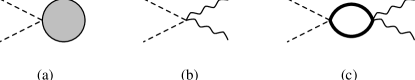
FIG. 4.: The initial term $\Delta$ is generated by diagrams of the form (a). The tree diagrams in (b) give the leading order contribution for small $n_{0}$. The leading order corrections come from the diagrams (c). For $\Delta^{(2,0)}$ the same diagrams would be used, but with the opposite sign for the $\lambda_{2}$ vertex on the left.

The diagrams which must be considered in calculating an effective initial term $(\Delta/2)\bar{\psi}^{2}$ are all those in which two $\psi$ lines exit from the left, as shown in Fig. 4(a). The sum of these diagrams gives rise to an effective term $f(t)\bar{\psi}(t)^{2}$ in the action. If the function $f(t)$ goes to zero for large $t$, and is sharply peaked enough that $\int_{0}^{\infty}dtf(t)$ is finite, then a coarse-graining in time gives $f(t)\bar{\psi}(t)^{2}\to(\Delta/2)\delta(t)\bar{\psi}(0)^{2}$, where both quantities are understood to be integrated over $t$, and $\Delta=2\int_{0}^{\infty}dt^{\prime}f(t^{\prime})$. To calculate this parameter $\Delta$ we consider first the subset of diagrams given by the tree diagrams, as shown in Fig. 4(b). These diagrams sum to give $f_{0}(t)=-\lambda_{2}/(1+n_{\phi}\lambda_{1}t)^{2}$, and so

$$\Delta_{0}=-2\lambda_{2}\int_{0}^{\infty}dt{1\over(1+n_{\phi}\lambda_{1}t)^{2}}=2n_{\phi}{\lambda_{2}\over\lambda_{1}}.$$ (44)

Therefore we conclude that this set of diagrams generates an effective initial term $\Delta_{0}=2n_{\phi}\lambda_{2}/\lambda_{1}$, or, in terms of the parameters in the master equation (10), $\Delta_{0}=n_{0}$, the initial density of each species. This will be shown to be the leading order term for a small $n_{0}$ expansion of $\Delta$. The width of the function $f_{0}(t)$ is given by $(n_{\phi}\lambda_{1})^{-1}$, and therefore we expect this coarse-grained picture to be valid for times $t\gg(n_{\phi}\lambda_{1})^{-1}$.

We can group all the diagrams in the full theory (34) which are of the form specified in Fig. 4(a) in the following way. There is a vertex $\lambda_{2}$ which is the leftmost vertex in the diagram. The lines coming into this vertex from the right can either come from mutually distinct or connected diagrams. The tree diagrams are a subset of the former group, and we argue that by letting $\lambda_{1}$ go to some bulk effective coupling $\lambda_{\rm eff}$ all diagrams of the former group are included. The connected diagrams can be grouped by the number of times they are connected, and shown in Fig. 4(c) are a set of diagrams which are connected exactly once. Again we argue that by taking $\lambda_{1}\rightarrow\lambda_{\rm eff}$ the diagrams of Fig. 4(c) give the entire contribution of the set which are connected exactly once. The sum of these diagrams is evaluated in the appendix, and is found to contribute to $\Delta$ a term which is higher order in $n_{0}$ than that given by the tree diagrams. It can be shown in general that the groups with more connections will contribute correspondingly higher order terms, and therefore this classification scheme gives rise to an expansion for $\Delta$.

Of course, an almost identical mechanism will also generate a term $\Delta^{(2,0)}\bar{\phi}(0)^{2}$, and it is straightforward to show on the grounds of symmetry that $\Delta^{(2,0)}=-\Delta$. Although this initial term is equally relevant from the renormalization group point of view, nevertheless it does not affect the late time behavior of the density. This is because it acts as a source for late time fluctuations only through the response function (38), and this is strongly damped for $t_{2}\gg t_{1}$. In contrast the response function of the $\psi$ field is simply the diffusion propagator, which has no such damping.

In summary of the discussion above, for $2<d\leq 4$ and for large times one can replace the full theory with a simplified action

$$S=\int d^{d}x\biggl{[} \int_{0}^{t}dt\Bigl{\{}\bar{\phi}(\partial_{t}-\nabla^{2})\phi+\bar{\psi}(\partial_{t}-\nabla^{2})\psi$$ (47)

$$-\lambda_{\rm eff}\bar{\phi}(\phi^{2}-\psi^{2})\Bigr{\}}-n_{\phi}\bar{\phi}(0)-{\Delta\over 2}\bar{\psi}(0)^{2}$$

$$+\hbox{other initial terms}\biggr{]},$$

where $\Delta$ is given by (6). Since the bulk theory, the terms within curly braces, is linear in $\bar{\phi}$ and $\bar{\psi}$ these fields can be integrated out to yield the equations of motion

$${\partial\over\partial t}\phi=\nabla^{2}\phi-\lambda_{\rm eff}\phi^{2}+\lambda_{\rm eff}\psi^{2}$$ (48)

$${\partial\over\partial t}\psi=\nabla^{2}\psi.$$ (49)

These are equations for classical fields with fluctuations in the initial conditions. They are often taken to be the continuum limit of the master equation (10), but we stress that only for $d>2$ and large times are these equations valid. In addition, since $\lambda_{\rm eff}<\lambda$, it is never correct to say that $\langle ab\rangle\sim\langle a\rangle\langle b\rangle$, but only that they are effectively proportional.

III Density Calculation for Equal Diffusion Constants

A Effective action: $2<d<4$

Starting with the action (47) one can calculate exactly the leading time dependence of the density, as well as correlation functions. We begin with a comment about notation. For this section and the next, where we deal with only the effective field theory, averages over the initial conditions will be denoted by angular brackets. The classical fields $\phi,\psi$ themselves represent bulk averages, or equivalently, averages over reaction and diffusion, of the same fields as written in (34). Also, the effective coupling is abbreviated to be $\lambda=\lambda_{\rm eff}$. With this notation, then, the average of equation (48) over the translationally invariant initial conditions is

$${d\over dt}\langle\phi\rangle=-\lambda\langle\phi^{2}\rangle+\lambda\langle\psi^{2}\rangle,$$ (50)

since $\nabla^{2}\langle\phi\rangle=0$.

FIG. 5.: Diagrammatic expansion for $\langle\phi\rangle$. Diagrams which contain initial terms other than $n_{\phi}$ and $\Delta$ are not shown, but are included in the sum. The only diagram in which the leftmost vertex is connected to $\psi$ fields is that of the single $\psi$ loop.

A diagrammatic expansion for $\langle\phi\rangle$ is shown in Fig. 5. Operating on both sides of this expansion with $(\partial_{t}-\nabla^{2})$, the inverse of the Green’s function propagator, gives equation (50). At this point, knowing that $\Delta$ is relevant for $d<4$, one might attempt to apply the renormalization group to try to find a nontrivial fixed point of order $4-d$. However, no such fixed point exists. This is because there are no corrections to a correlation function $\langle\psi(x_{1},t_{1})\psi(x_{2},t_{2})\bar{\psi}(0)^{2}\rangle$, so that $\Delta$ is not renormalized. It therefore flows, for $d<4$, to infinity under renormalization. This would appear to make it very difficult to sum the diagrams in Fig. 5 explicitly. However, it turns out to be possible to solve (50) exactly for late times. There is only one diagram contributing to the value of $\langle\psi^{2}\rangle$ in equation (50), which is the single $\psi$ loop. Evaluating this loop gives $\langle\psi^{2}\rangle=\Delta/(8\pi t)^{d/2}$. It is important to note that this result holds even when all possible higher order initial terms are included.

Next, consider a related problem in which $\langle\phi^{2}\rangle$ in (50) is replaced by $\langle\phi\rangle^{2}$, which is equivalent to including only the diagrams in Fig. 5 which are disconnected to the right of the leftmost vertex. This partial sum satisfies a differential equation known as Ricatti’s equation, which, though non-linear, can be solved. Let $f$ denote the function which satisfies this equation, that is,

$${d\over dt}f=-\lambda f^{2}+\lambda{\Delta\over(8\pi)^{d/2}}t^{-d/2}.$$ (51)

It will be shown below that this function $f$ provides a upper bound for the actual density, but first we will discuss the solution of this equation. It is integrable for certain values of $d$, specifically $d=4$ and $d=4\pm 4/(2s+1)$ where $s$ is a non-negative integer. For general values of $d$ a solution can be obtained by transforming the equation via the substitution $f=\dot{u}/(\lambda u)$, which gives

$$\ddot{u}={\lambda^{2}\Delta\over(8\pi)^{d/2}}t^{-d/2}u,$$ (52)

a linear, second order equation whose solution can be expressed in terms of confluent hypergeometric functions. Therefore the asymptotic behavior of $f$ is rigorously obtained, and is in fact what one naively obtains by assuming $f\sim At^{-\alpha}$ and inserting it into (51):

$$f\sim\cases{\Delta^{1/2}(8\pi t)^{-d/4}&$d<4$\cr A_{4}^{u}\>t^{-1}&$d=4$\cr(\lambda t)^{-1}&$d>4$.\cr}$$ (53)

When $d<4$ the asymptotic behavior comes from balancing the two terms on the right hand side of (51), whereas for $d>4$ it comes from balancing the $f^{2}$ and the $\dot{f}$ terms. For $d=4$ all three terms contribute, and the amplitude is

$$A_{4}^{u}={1\over 2\lambda}+\sqrt{{1\over(2\lambda)^{2}}+{\Delta\over(8\pi)^{2}}}.$$ (54)

The case of $d=4$ will be discussed in more detail in section III B. Notice that the asymptotic behavior of the solution $f$ is independent of the initial conditions. In fact, the initial conditions must be specified at some $t_{0}>0$, since the equation is singular at $t=0$. A natural choice for this initial time is that given by the coarse-graining time scale of the effective initial conditions, that is $t_{0}=(n_{\phi}\lambda)^{-1}$.

Now we show that $f$ provides an upper bound for the actual density $\langle\phi\rangle$. Our method is to derive an equation for $\chi=f-\langle\phi\rangle$ and show that asymptotically $\chi\geq 0$. Since $\phi$ is a real field in the effective theory, then $h(t)\equiv\langle\phi^{2}\rangle-\langle\phi\rangle^{2}\geq 0$. Equation (50) can be rewritten

$${d\over dt}\langle\phi\rangle=-\lambda h(t)-\lambda\langle\phi\rangle^{2}+\lambda\langle\psi^{2}\rangle,$$ (55)

and then substituting $\langle\phi\rangle=f-\chi$ gives

$${d\over dt}\chi=\lambda h+\lambda(\chi-2f)\chi.$$ (56)

Assume that $\chi(t_{0})=0$, that is we choose the initial condition for $f$ such that $f(t_{0})=\langle\phi(t_{0})\rangle$. As mentioned above, the asymptotic value of $f$ is independent of the choice of initial conditions. Since $f$ is known to be positive for all $t>t_{0}$, then from equation (56) we know that $\dot{\chi}>0$ whenever $\chi<0$. Now suppose that there exists some $t_{1}>t_{0}$ for which $\chi(t_{1})<0$. Since $\chi(t)$ is a continuous function, it follows that there must be some intermediate time $t_{0}<t<t_{1}$ for which $\chi(t)<0$ and $\dot{\chi}(t)<0$. This is in contradiction with equation (56), and therefore our assumption that there exists $\chi(t_{1})<0$ for $t_{1}>t_{0}$ is false.

We can also find a lower bound for $\langle\phi\rangle$ by noting that $\phi({\bf x},t)\geq|\psi({\bf x},t)|$ at all points $({\bf x},t)$. This is equivalent to the statement that $a({\bf x},t),b({\bf x},t)$ are at all points non-negative, when starting from any initial condition in which $a,b$ are everywhere non-negative. While this result is somewhat intuitive, it can be made more rigorous by considering the field equations (48), (49) expressed in terms of $a=(\phi+\psi)/\sqrt{2}$ and $b=(\phi-\psi)/\sqrt{2}$:

$${\partial\over\partial t}a=\nabla^{2}a-\sqrt{2}\lambda ab\qquad\qquad{\partial\over\partial t}b=\nabla^{2}b-\sqrt{2}\lambda ab.$$ (57)

Given that the fields $a,b$ are initially everywhere non-negative, then for the fields to have a negative value at a later time $t_{1}$ there must be an intermediate time $0<t_{0}<t_{1}$ for which both $a(t_{0})=0$ and $\partial_{t}a(t_{0})<0$. However, in the case where $a=0$ at a single point in space, then $a>0$ locally around the point, implying that it is a local minimum and $\partial_{t}a>0$. For a region of $a=0$ equation (57) gives $\partial_{t}a=0$ in the region and $\partial_{t}a>0$ on the boundary. Therefore the fields cannot pass through zero, and will remain non-negative.

Since $\phi\geq|\psi|$ it follows that $\langle\phi\rangle\geq\langle|\psi|\rangle$. At late times $\psi$ has a normal distribution, independent of the initial distribution, which follows from the fact that $\psi$ obeys the simple diffusion equation (49). Therefore the asymptotic value of $\langle|\psi|\rangle$ can be computed directly. The asymptotic distribution of $\psi$ is given by

$$P[\psi(t)]\propto\exp\left\{-{\psi(t)^{2}\over 2\langle\psi(t)^{2}\rangle}\right\},$$ (58)

from which it follows that

$$\langle|\psi(t)|\rangle=\sqrt{{2\over\pi}\langle\psi(t)^{2}\rangle}={(2\Delta)^{1/2}\over\pi^{1/2}(8\pi)^{d/4}}t^{-d/4}.$$ (59)

Given the upper bound $\langle\phi\rangle\leq f\sim O(t^{-d/4})$ it can be shown that $\langle\phi\rangle\sim\langle|\psi|\rangle$, that is, that the lower bound gives exactly the density. Since $\langle g^{2}\rangle\geq\langle g\rangle^{2}$ for any real $g$, then

$$\langle\phi-|\psi|\rangle^{2}\leq\langle(\phi-|\psi|)^{2}\rangle=\langle\phi^{2}\rangle+\langle\psi^{2}\rangle-2\langle\phi|\psi|\rangle$$ (60)

Using again $\phi\geq|\psi|$:

$$\langle\phi-|\psi|\rangle^{2}\leq\langle\phi^{2}\rangle-\langle\psi^{2}\rangle=-{1\over\lambda}\langle\dot{\phi}\rangle=O(t^{-1-d/4}).$$ (61)

Therefore $\langle\phi\rangle=\langle|\psi|\rangle+O(t^{-1/2-d/8})$, which gives $\langle\phi\rangle\sim\langle|\psi|\rangle$ for $d<4$. This is actually a statement about segregation in the system, implying that to leading order the density of $a+b$ is the same as $|a-b|$, or equivalently, that the minority species in each region decays faster than the majority. For $2<d<4$ then, we find

$$\langle a\rangle\sim{\Delta^{1/2}\over\pi^{1/2}(8\pi)^{d/4}}t^{-d/4},$$ (62)

as stated in section I, with $\Delta$ given by (6). Substituting the leading order term in the expansion $\Delta=n_{0}+O(n_{0}^{d/2})$ then gives the result of Toussaint and Wilczek [4]. In fact, our method is very similar to theirs, with two exceptions. First, they use a central limit argument to calculate $\Delta$, whereas we can compute it directly from the full field theory. It is reassuring that the answers agree, to leading order in $n_{0}$. The other difference is that they calculate $\langle|\psi|\rangle$, and then hypothesize the asymptotic segregation, saying $\langle\phi\rangle\sim\langle|\psi|\rangle$. Starting from the effective theory (47) we have shown rigorously that these quantities are asymptotically the same.

B Effective Action: $d\geq 4$

When $d=4$ the upper and lower bounds for the density from section III A still hold: $\langle|\psi|\rangle\leq\langle\phi\rangle\leq f$. However, it is no longer necessarily true that $\langle\phi\rangle\sim\langle|\psi|\rangle$, since the bound on the corrections, which is of order $O(t^{-1/2-d/8})$, is the same order as the density. The upper bound $\langle\phi\rangle\leq f\sim A_{4}^{u}/t$ is given by (53) and (54). Notice that for small $\lambda$ or small $\Delta$ that $A_{4}^{u}\rightarrow 1/\lambda$. Also, when $\lambda$ is large or $\Delta$ is large then $A_{4}^{u}\rightarrow\Delta^{1/2}/(8\pi)$. However, in the intermediate region there is a smooth crossover in the upper bound from the $\lambda$ dependent asymptote to the $\Delta$ dependent asymptote.

The lower bound is given by $\langle\phi\rangle\geq\langle|\psi|\rangle=A_{4}^{\ell}/t$ with $A_{4}^{\ell}=\Delta^{1/2}/8\pi^{3/2}$. For large $\Delta$, then, the upper and lower bounds differ by a factor of $\sqrt{\pi}$. The lower bound continues to decrease with $\Delta$, and therefore is not very useful in the small $\Delta$ limit. However, since the parameter $\Delta$ is dimensionless in $d=4$ one can do a perturbative expansion for small $\Delta$, which results in a better lower bound. It follows from equation (50) that the zeroth order term in this expansion is a constant, and is in fact equal to the small $\Delta$ limit of the upper bound, $\lambda^{-1}$. To the next order one has

$$\langle a\rangle={1\over\lambda t}+{\lambda\Delta\over t}+O(\Delta^{2}),$$ (63)

and it is plausible to conjecture that the amplitude is monotonically increasing with $\Delta$.

The amplitude given by Bramson and Lebowitz [6], has the form

$$A_{4}\propto\cases{\hbox{constant}&$\Delta<\Delta_{c}$\cr\Delta^{1/2}&$\Delta>\Delta_{c}$,\cr}$$ (64)

that is, the amplitude is independent of $\Delta$ for small $\Delta$. Their result seems to be at odds with our small $\Delta$ calculation. However, as discussed in section II, there are differences between our model and the one they study. Since the corrections to the small $n_{0}$ or $\Delta$ limit are non-universal, this is a possible explanation of the discrepancy.

When $d>4$ then it follows from the power counting of section II C that the $(\Delta/2)\bar{\psi}^{2}$ initial term is irrelevant. In this case the density is given asymptotically by $\langle a\rangle\sim(\lambda t)^{-1}$. The power law of the density decay is independent of the dimension of space. The amplitude $\lambda^{-1}$ will depend on the dimension and the microscopic details, but it is independent of initial terms, or equivalently initial conditions.

C Renormalization for $d\leq 2$

When $d\leq 2$ one has to consider the full theory as given by the action (34), and the subsequent renormalization. Although (50) is still valid formally, since the noise in (41) averages to zero, we can no longer apply the upper and lower bounds of the previous section since, in the presence of the imaginary noise term, $\phi$ is no longer real.

Much of the contents of this section is directly related to the one-species calculation of Ref. [13], in which more details can be found. The primitively divergent vertex functions were identified by power counting in section II B, and were found to be those with two lines coming in and two or fewer lines going out. These primitive divergences are used to define a renormalized coupling, following conventional RG methods [22]. It is found that all the vertices in the action (34) renormalize identically, with the primitive divergences given by the bubble sums shown in Fig. 6.

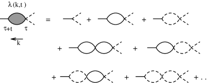
FIG. 6.: The sum of diagrams which contribute to the primitively divergent vertex function $\lambda_{i}(k,t)$. Shown here is the case $i=1$, with the $\psi$ propagators for the incoming external legs.

In this sum all diagrams of a given number of loops come in with the same sign, since replacing a $\phi$ loop with a $\psi$ loop, for example, introduces always two negative signs (see Fig. 1). At the order of $n$ loops there are $2^{n}$ diagrams, so these form a geometric sum, with the ratio given by $2$ times the value of a single loop. Denoting this sum by $\lambda_{i}(k,t)$ where $i=1,2$ labels the number of outgoing lines, then the Laplace transform, $\lambda_{i}(k,s)=\int_{0}^{\infty}dt\>e^{-st}\lambda_{i}(k,t)$ is given by

$$\lambda_{i}(k,s)={\lambda_{i}\over 1+[4/(8\pi)^{d/2}]\,\lambda_{2}\,\Gamma(\epsilon/2)(s+k^{2}/2)},$$ (65)

where $\epsilon=2-d$. The renormalized coupling is defined in terms of an arbitrary normalization scale $\kappa$, which has dimensions of wave number: $g_{R}=\kappa^{-\epsilon}\lambda_{2}(k=0,s=\kappa^{2})$. Then the $\beta$ function is

$$\beta(g_{R})=\kappa{\partial\over\partial\kappa}g_{R}=-\epsilon g_{R}+{4\epsilon\over(8\pi)^{d/2}}\Gamma\left(\epsilon\over 2\right)g_{R}^{2}$$ (66)

which gives a fixed point $g_{R}^{*}=O(\epsilon)$.

Let the density $n(t)=\langle a(t)\rangle=\langle b(t)\rangle$. Since the density is independent of the normalization scale, then $dn/d\kappa=0$, which leads to the Callan-Symanzik equation

$$\biggl{[}2t{\partial\over\partial t}- dn_{\phi}{\partial\over\partial n_{\phi}}-d\Delta{\partial\over\partial\Delta}+\beta(g_{R}){\partial\over\partial g_{R}}+d\biggr{]}n(t,g_{R},n_{\phi},\Delta)$$ (68)

$$=0.$$

The solution is found by the method of characteristics to be

$$n(t,g_{R},n_{\phi},\Delta)=(\kappa^{2}t)^{-d/2}n(\kappa^{-2},\tilde{g}_{R},\tilde{n}_{\phi},\tilde{\Delta}),$$ (69)

where in the asymptotic limit of large $\kappa^{2}t$ the running coupling has the limit $\tilde{g}_{R}\rightarrow g_{R}^{*}$. However, the running initial couplings go as $\tilde{n}_{\phi}=n_{\phi}(\kappa^{2}t)^{d/2}$ and $\tilde{\Delta}=\Delta(\kappa^{2}t)^{d/2}$, that is, they flow to a strong coupling limit.

The solution (69) is used to calculate the asymptotic density in the following way: the density is calculated as an expansion in $g_{R}$ and $n_{\phi}$, and this expansion is put into the right-hand side of (69). Then, in the limit of large $\kappa^{2}t$, the coupling expansion will yield an $\epsilon$ expansion, but only if the behavior at large $\tilde{n}_{\phi}$ and $\tilde{\Delta}$ is controlled. This may be done if the diagrams may be grouped into sums over all powers of $\tilde{n}_{\phi}$ and $\tilde{\Delta}$, which, when summed, yield a well-defined limit. In the one-species case this grouping was relatively simple. The series may be put in the form of a sum of terms $g_{R}^{n}\tilde{n}_{\phi}f_{n}(g_{R}\tilde{n}_{\phi})$, where $n$ counts the number of loops in a given diagram. The term $n=0$ corresponds to the sum of tree diagrams, given by the solution of the simple rate equation, so that $f_{0}(g_{R}\tilde{n}_{\phi})\propto(g_{R}\tilde{n}_{\phi})^{-1}$ as $\tilde{n}_{\phi}\to\infty$. By explicit calculation, it is then possible to show that the $f_{n}$ for $n>0$ behave in a similar manner. Since $g_{R}\to g_{R}^{*}=O(\epsilon)$, this lead to the result that $n(t)\sim A/t^{d/2}$ where the amplitude $A$ is in principle calculable to any order in $\epsilon$. In the present case, the series may similarly be organized as a sum of terms of the form $g_{R}^{n}\tilde{n}_{\phi}f_{n}(g_{R}\tilde{n}_{\phi},g_{R}^{2}\tilde{\Delta})$, where now the $n=0$ term is given by the sum of diagrams in Fig. 5. This is given by the solution of (50), which, by the analysis of the previous section, implies that $f_{0}(g_{R}\tilde{n}_{\phi},g_{R}^{2}\tilde{\Delta})\propto(g_{R}^{2}\tilde{\Delta})^{1/2}/(g_{R}\tilde{n}_{\phi})$ in this limit. However, unlike the single species case, $n$ does not simply count the loops, since already at $n=0$ there are arbitrarily many $\psi$ loops. In addition, while it is possible to identify those diagrams appearing at $n=1$ for example, it is difficult to see how to express their sum in terms of a suitable generalization of (50), and thereby evaluate it. Assuming that their asymptotic behavior is independent of $n_{0}$ and thus of $\tilde{n}_{\phi}$, there are three conceivable ways in which these higher order terms could affect the result. They either diverge less slowly than ${\tilde{\Delta}}^{1/2}$ as $\tilde{\Delta}\to\infty$, in which case the $n=0$ result gives the leading behavior, which would then yield the same result as for $d>2$; or they all behave like ${\tilde{\Delta}}^{1/2}$, in which case the density behaves as $t^{-d/4}$ but with an amplitude which has a nontrivial expansion in powers of $\epsilon$; or they diverge more strongly, in which case the density no longer behaves as $t^{-d/4}$ for $d<2$. Since this last possibility is in conflict with numerical experiments and rigorous results (albeit for slightly different models), it is unlikely to be correct.

When $d=2$ the running coupling goes to zero as $(\ln t)^{-1}$ for $t\rightarrow\infty$, rather than to an order $\epsilon$ fixed point. Therefore the leading order terms for an $\epsilon$ expansion of the amplitude become the exact asymptotic amplitude, with correction terms which go as $(\ln t)^{-1}$. Therefore, if our conjecture is correct, then density should be given exactly by (62) in the large $t$ limit.

IV Density Calculation for Unequal Diffusion Constants

When the two species of particles no longer have equal diffusion constants, then the vertices which depend on $\delta$ must be included in the full theory. Then for $d>2$ an effective theory can be developed, just as before, with the resulting action

$$S=\int d^{d}x\biggl{[} \int_{0}^{t}dt\Bigl{\{}\bar{\phi}(\partial_{t}-\nabla^{2})\phi+\bar{\psi}(\partial_{t}-\nabla^{2})\psi-\bar{\psi}\delta\nabla^{2}\phi$$ (72)

$$-\bar{\phi}\delta\nabla^{2}\psi+\lambda\bar{\phi}(\phi^{2}-\psi^{2})\Bigr{\}}-n_{\phi}\bar{\phi}(0)-{\Delta\over 2}\bar{\psi}(0)^{2}$$

$$+\dots\biggr{]}.$$

The effective theory describes classical fields which evolve via the deterministic equations of motion

$${\partial\over\partial t}\phi=\nabla^{2}\phi+\delta\nabla^{2}\psi-\lambda\phi^{2}+\lambda\psi^{2}$$ (73)

$${\partial\over\partial t}\psi=\nabla^{2}\psi+\delta\nabla^{2}\phi,$$ (74)

which follows from integrating out the $\bar{\phi},\bar{\psi}$ degrees of freedom in the bulk component of (72). From these equations the density can be calculated exactly by using the same methods as before. First, equation (73) is averaged over the initial conditions to yield equation (50), just as in the $\delta=0$ case. The solution to Ricatti’s equation again provides an upper bound $\langle\phi\rangle\leq f\sim\sqrt{\langle\psi(t)^{2}\rangle}$, although the value of $\langle\psi(t)^{2}\rangle$ is changed. It will be shown that $\langle\psi^{2}\rangle\propto t^{-d/2}$, so the upper bound decays with the same exponent as before. Since the fields are real and $\phi\geq|\psi|$, it then follows that $\langle\phi\rangle\sim\langle|\psi|\rangle$ for $d<4$, as shown in (61). Furthermore, it will be shown that asymptotically $\psi(t)$ has a normal distribution, so the density is given exactly by $\langle a\rangle=\langle\phi\rangle/\sqrt{2}\sim\sqrt{\langle\psi^{2}\rangle/\pi}$. Therefore the only change in the asymptotic density from the $\delta=0$ case is due to the change in the value of $\langle\psi(t)^{2}\rangle$.

A Calculation of $\langle\psi(t)^{2}\rangle$

The initial terms in the effective theory are in general changed by the presence of $\delta$ in the full theory, and therefore must be computed again. One can show that, as before, no $\Delta^{(0,1)}\bar{\psi}$ initial term is generated. For any diagram which ends with a single $\psi$ line, the last vertex (first from the left) must be a $\delta k^{2}$ vertex. However, this external line has $k=0$, and so all of these diagrams have no contribution. To leading order $\Delta=n_{0}$ is unchanged, as can be seen from the diagrams in Fig. 4: the leading order contribution to $\Delta$ comes from diagrams composed of no loops, and so all lines carry wave number $k=0$ and are unaffected by the $\delta k^{2}$ vertex. The correction terms to the small $n_{0}$ limit of $\Delta$ will likely be of the same order as before, $O(n_{0}^{d/2}\lambda^{d/2})$, but with a different amplitude. This amplitude could be calculated, although it would require a generalization of the response functions discussed below. It will be shown the asymptotic value of $\langle\psi^{2}\rangle$ depends only on $\Delta$, and so the other surface terms can be neglected.

There are new response functions generated in the bulk theory. With $\delta=0$ there was just a bare $\psi$ propagator and a $\phi$ response function. In this theory there are instead four response functions, which connect $\phi,\psi$ to $\bar{\phi},\bar{\psi}$ in each possible way, as shown in Fig. 7. Each of these response functions, represented by double lines, is an infinite sum over all possible numbers of $\delta k^{2}$ vertices inserted.

FIG. 7.: The response functions for the case $\delta\neq 0$, and the coupled equations they satisfy.

These response functions can be found exactly via coupled integral equations, also shown in Fig. 7. For our purposes, since just the leading term for small $n_{0}$ is being calculated, we need only the form of the response functions when the earlier time argument is set to zero. To calculate the higher order terms in the expansion $\Delta=n_{0}+\dots$ one needs to derive these response functions with $t_{1}\neq 0$. Setting $t_{2}=t$, $t_{1}=0$ in the equations represented by diagrams (a) gives

$$G(k,t)=e^{-k^{2}t}+\delta k^{2}\int_{0}^{t}dt^{\prime}e^{-k^{2}(t-t^{\prime})}F(k,t^{\prime})$$ (75)

$$F(k,t)=\delta k^{2}\int_{0}^{t}dt^{\prime}e^{k^{2}(t-t^{\prime})}\left(1+n_{\phi}\lambda t^{\prime}\over 1+n_{\phi}\lambda t\right)^{2}G(k,t^{\prime}),$$ (76)

or, in terms of $f,g$ defined by $G(k,t)=e^{-k^{2}t}g(k,t)$ and $F(k,t)=e^{-k^{2}t}f(k,t)$

$$g(k,t)=1+\delta k^{2}\int_{0}^{t}dt^{\prime}f(k,t^{\prime})$$ (77)

$$f(k,t)=\delta k^{2}\int_{0}^{t}dt^{\prime}\left(1+n_{\phi}\lambda t^{\prime}\over 1+n_{\phi}\lambda t\right)^{2}g(k,t^{\prime}).$$ (78)

Differentiating equations (77) and (78) with respect to $t$ gives

$$f(k,t)={1\over\delta k^{2}}\dot{g}(k,t)$$ (79)

$${\partial\over\partial t}\left[(1+n_{\phi}\lambda t)^{2}f(k,t)\right]=\delta k^{2}(1+n_{\phi}\lambda t)^{2}g(k,t)$$ (80)

Substituting for $f$ into the lower equation and manipulating the expression gives a remarkably simple equation for $g$

$${\partial^{2}\over\partial t^{2}}[(1+n_{\phi}\lambda t)g]=\delta^{2}k^{4}[(1+n_{\phi}\lambda t)g]$$ (81)

which has the general solution

$$g(k,t)={1\over 1+n_{\phi}\lambda t}\left[A\cosh(\delta k^{2}t)+B\sinh(\delta k^{2}t)\right].$$ (82)

From the integral equation (77) one finds the conditions $g(k,0)=1$, which implies $A=1$, and $g(0,t)=1$, which then implies $B=n_{0}\lambda/(\delta k^{2})$. Therefore the explicit form of $G(k,t)$, and from (79) $F(k,t)$, is calculated:

$$G(k,t)={e^{-k^{2}t}\over 1+n_{\phi}\lambda t}\left[\cosh(\delta k^{2}t)+{n_{\phi}\lambda\over\delta k^{2}}\sinh(\delta k^{2}t)\right],$$ (83)

$$F(k,t)={e^{-k^{2}t}\over(1+n_{\phi}\lambda t)^{2}} \biggl{[}\biggl{(}1+n_{\phi}\lambda t-{n_{\phi}^{2}\lambda^{2}\over\delta^{2}k^{4}}\biggr{)}\sinh(\delta k^{2}t)$$ (85)

$$+{n_{\phi}^{2}\lambda^{2}t\over\delta k^{2}}\cosh(\delta k^{2}t)\biggr{]}.$$

The other response functions, $H(k,t)$ and $J(k,t)$, defined in diagram Fig. 7, can be found via similar methods. The coupled integral equations shown in Fig. 7(b), written in terms of $h=e^{k^{2}t}H$ and $j=e^{k^{2}t}J$, are

$$h(k,t)={1\over(1+n_{\phi}\lambda t)^{2}}+\delta k^{2}\int_{0}^{t}dt^{\prime}\left(1+n_{\phi}\lambda t^{\prime}\over 1+n_{\phi}\lambda t\right)^{2}j(k,t^{\prime})$$ (86)

$$j(k,t)=\delta k^{2}\int_{0}^{t}h(k,t^{\prime}).$$ (87)

Differentiating both equations with respect to $t$ and substituting to eliminate $h$ gives the equation

$${\partial^{2}\over\partial t^{2}}[(1+n_{\phi}\lambda t)j]=\delta^{2}k^{4}[(1+n_{\phi}\lambda t)j]$$ (88)

which has the general solution

$$j(k,t)={1\over 1+n_{\phi}\lambda t}\left[A\cosh(\delta k^{2}t)+B\sinh(\delta k^{2}t)\right].$$ (89)

The condition that $j(k,0)=0$ implies $A=0$. The general solution of $h$ can be found from (89), and then the condition that $h(k,0)=1$ implies $B=1$. Therefore $H$ and $J$ are given by

$$H(k,t)={e^{-k^{2}t}\over(1+n_{\phi}\lambda t)^{2}} \biggl{[}(1+n_{\phi}\lambda t)\cosh(\delta k^{2}t)$$ (91)

$$-{n_{\phi}\lambda\over\delta k^{2}}\sinh(\delta k^{2}t)\biggr{]}$$

$$J(k,t)={e^{-k^{2}t}\over(1+n_{\phi}\lambda t)}\sinh(\delta k^{2}t).$$ (92)

FIG. 8.: The generalization of the simple $\psi$ loop of Fig. 5 to the case of $\delta\neq 0$.

In section III A the value of $\langle\psi^{2}\rangle$ was calculated from the simple loop shown in Fig. 5. The generalization of this calculation is given by the diagrams shown in Fig. 8, which are composed of the $G(k,t)$ and $J(k,t)$ response functions. The surface couplings $\Delta^{(0,2)}\neq-\Delta^{(2,0)}$ beyond the leading small $n_{0}$ terms, and so the couplings are labeled $\Delta$ and $\Delta^{\prime}$ respectively. It should be noted that unlike the $\delta=0$ case, these are not the only diagrams which contribute to $\langle\psi^{2}\rangle$. Examples of other diagrams, and arguments for why they are irrelevant, will be given below. First, we compute those of Fig. 8, which give

$$\langle\psi(t)^{2}\rangle=\int{d^{d}k\over(2\pi)^{d}}[\Delta\,G(k,t)^{2}-\Delta^{\prime}J(k,t)^{2}].$$ (93)

Substituting (83) and (92) into the equation above, and rewriting the integral in terms of the variable $u=k^{2}t$ gives

$$\langle\psi(t)^{2}\rangle = {t^{-d/2}\over(4\pi)^{d/2}\Gamma(d/2)(1+n_{\phi}\lambda t)^{2}}\int_{0}^{\infty}du\>u^{d/2-1}e^{-2u}$$ (94)

$$\mbox{}\times \biggl{[}\Delta\cosh^{2}(\delta u)-\Delta^{\prime}\sinh^{2}(\delta u)+{\Delta n_{\phi}\lambda t\over\delta u}\sinh(2\delta u)$$ (96)

$$\mbox{}+\Delta\left(n_{\phi}\lambda t\over\delta u\right)^{2}\sinh(\delta u)^{2}\biggr{]}.$$

Each term in the square brackets gives a convergent integral for $d>0$. Therefore we can take the large $t$ limit before integrating, and only calculate the leading term in $t$, which is found to be that on the far right in the brackets. Consequently, the value of $\Delta^{\prime}$ is unimportant.

Evaluating this integral gives

$$\langle\psi^{2}\rangle={\Delta\over(8\pi)^{d/2}}Q(d,\delta)\>t^{-d/2}$$ (97)

where

$$Q(d,\delta)={4\left[(1+\delta)^{2-d/2}+(1-\delta)^{2-d/2}-2\right]\over\delta^{2}(d-2)(d-4)}.$$ (98)

From (97) it follows that $Q\sim\langle\psi^{2}\rangle_{\delta}/\langle\psi^{2}\rangle_{0}$, in the small $n_{0}$ limit. This function $Q$ is non-singular at $\delta=0$, and satisfies $Q(d,0)=1$. While $Q$ appears to be divergent at $d=2,4$, it is actually finite everywhere except $d\geq 4$ and $\delta=\pm 1$. It is likely that the limits of $t\rightarrow\infty$ and $\delta\rightarrow\pm 1$ do not necessarily commute, and that a separate treatment for the case of an immobile species, at least in this singular case, would be required. For $d<4$ this function has finite values as $\delta\rightarrow\pm 1$, but the slope at $\delta=\pm 1$ is infinite for $d\geq 2$.

FIG. 9.: A plot of $\sqrt{Q}=\langle a\rangle_{\delta}/\langle a\rangle_{0}$ for integer values of $d$.

While the calculation of $Q(d,\delta)$ is only strictly valid for $2<d<4$, it is nonetheless interesting to consider its limits for the integer dimensions from $d=1$ to $d=4$, motivated by section III C on $d\leq 2$, in which it was conjectured that the “classical” amplitude is also the leading term in an $\epsilon$ expansion for $d=2-\epsilon$. From (98)

$$Q(d,\delta)=\cases{{\displaystyle 4\over\displaystyle 3\delta^{2}}[(1+\delta)^{3/2}+(1-\delta)^{3/2}-2]&$d=1$\cr\vskip 6.0pt plus 2.0pt minus 2.0pt\cr{\displaystyle(1-\delta)\ln(1-\delta)+(1+\delta)\ln(1+\delta)\over\displaystyle\delta^{2}}&$d=2$\cr\vskip 6.0pt plus 2.0pt minus 2.0pt\cr{\displaystyle 4\over\displaystyle\delta^{2}}[2-\sqrt{1+\delta}-\sqrt{1-\delta}]&$d=3$\cr\vskip 6.0pt plus 2.0pt minus 2.0pt\cr{\displaystyle-\ln(1-\delta^{2})\over\displaystyle\delta^{2}}&$d=4$\cr}$$ (99)

Since the density goes as $\sqrt{\langle\psi^{2}\rangle}$, the function $\sqrt{Q(d,\delta)}$ is plotted in Fig. 9 for integer values of $d$. The density amplitude increases monotonically with $|\delta|$, but is not changed remarkably for modest values of $\delta$.

FIG. 10.: (a) An example of one of the diagrams besides those of Fig. 8 which contribute to $\langle\psi^{2}\rangle$, and (b) the effective bulk vertices that all such diagrams contain.

There are other diagrams which give contributions to $\langle\psi^{2}\rangle$, unlike the $\delta=0$ case. Some of these are shown in Fig. 10(a). All of these diagrams have the similar feature that they contain one of the two sub-diagrams in Fig. 10(b). These sub-diagrams give rise to effective vertices of the form $\lambda^{\prime}\bar{\psi}\nabla^{2}\psi^{2}$ and $\lambda^{\prime}\bar{\psi}\nabla^{2}\phi^{2}$ in the bulk theory. However, such vertices are irrelevant, which follows from power counting, and so the diagrams which arise from them must be sub-leading in time. Therefore we conclude that asymptotically the value of $\langle\psi^{2}\rangle$ is given by (97) and (98).

B Demonstration that $\psi(t)$ has a Normal Distribution

In order for the calculation of $\langle\psi^{2}\rangle$ to give the amplitude of the density it is necessary that $\psi(t)$ have a normal distribution. When $\delta=0$ this follows directly from the simple diffusion equation satisfied by $\psi$, or equivalently, from central limit arguments. However, $\psi$ evolves via equation (74) for $\delta\neq 0$, and so it needs to be shown that it still flows to a normal distribution. What we will show is that the random variable $t^{d/4}\psi$ flows to a static normal distribution, the width of which was calculated above.

Consider $\langle\psi^{n}\rangle$, where $n$ is even. There is one diagram in which $n$ response functions $G(k,t)$ are connected in pairs to $n/2$ initial terms $(\Delta/2)\bar{\psi}^{2}$. This diagram contains $n/2$ loops, and is therefore of order $t^{-nd/4}$. It was shown above replacing any of the $G(k,t)$ loops with $J(k,t)$ response functions connected to $(\Delta^{\prime}/2)\bar{\phi}^{2}$ gives a lower order contribution. Similarly, any other diagrams, which would originate from considering higher order surface terms, will involve more than $n/2$ loops, and will therefore decay faster in time. For $n$ odd one finds that there are no diagrams for $\langle\psi^{n}\rangle$ which decay as slowly as $t^{-nd/4}$. That is, for $n$ odd, $\lim_{t\rightarrow\infty}\langle(t^{d/4}\psi)^{n}\rangle=0$. Since the distribution of the variable $t^{d/4}\psi$ has only even moments as $t\rightarrow\infty$, and these moments are just multiples of $\langle(t^{d/4}\psi)^{2}\rangle$, generated by all possible pair contractions, then the distribution is normal.

V Correlation Functions for $2<d<4$

When $d>2$, one can use the classical action to calculate the correlation functions. Consider the distribution of the random variable $t^{d/4}\phi({\bf x},t)$ with $2<d<4$. From section III A we know that $\langle t^{d/4}\phi-t^{d/4}|\psi|\rangle\rightarrow 0$ as $t\rightarrow\infty$. Furthermore, from equation (61) it follows that, as $t\rightarrow\infty$, $\langle(t^{d/4}\phi-t^{d/4}|\psi|)^{2}\rangle\rightarrow 0$. This suggests that the distributions $P[t^{d/4}\phi]\sim P^{\prime}[t^{d/4}|\psi|]$ as $t\rightarrow\infty$. The latter distribution is known exactly, as $t^{d/4}\psi$ is at late times given by a static normal distribution.

It is not correct to say that asymptotically $\phi$ and $|\psi|$ are everywhere equal, since this would imply that there are no regions in which the densities $a$ and $b$ are both non-zero. However, the reaction regions, those in which both densities are non-zero, become negligibly small for large $t$, and the corrections to setting $\phi$ equal to $|\psi|$ in calculating correlation functions will be subleading in time. Stated another way, the leading term in both $\langle\phi_{1}\phi_{2}\rangle$ and $\langle|\psi_{1}||\psi_{2}|\rangle$ is of order $t^{-d/2}$. To this order the two random variables $\phi$ and $|\psi|$ have identical distributions. This is in contrast to a quantity such as $\phi^{2}-\psi^{2}$, which is measuring a subleading term relative to $t^{-d/2}$.

We can use the property that $t^{d/4}\phi$ is given by the absolute value of a gaussian random field to calculate correlation functions. This is similar to what is done is the dynamics of phase ordering, where the order parameter field can be mapped to an auxiliary field which is assumed to be a gaussian random field. This analogy will be discussed further below.

Since $\phi$ and $|\psi|$ are given by the same distribution, we conclude $\langle\phi_{1}\phi_{2}\rangle\sim\langle|\psi_{1}||\psi_{2}|\rangle$, where the labels indicate the positions ${\bf x}_{1}$ and ${\bf x}_{2}$ at time $t$. The correlation function $\langle|\psi_{1}||\psi_{2}|\rangle$ can be calculated exactly by using the fact that, asymptotically, $\psi(t)$ has a normal distribution. The joint probability distribution $P[\psi_{1},\psi_{2}]$ is then also normal, so

$$P[\psi_{1},\psi_{2}]={\sqrt{4\alpha^{2}-\beta^{2}}\over 2\pi}\exp\left\{-\alpha\psi_{1}^{2}-\alpha\psi_{2}^{2}-\beta\psi_{1}\psi_{2}\right\},$$ (100)

where we have used translational invariance to set $\langle\psi_{1}^{2}\rangle=\langle\psi_{2}^{2}\rangle$. The constants $\alpha$ and $\beta$ are determined by the values of $\langle\psi^{2}\rangle$ and $\langle\psi_{1}\psi_{2}\rangle$, which are evaluated from the diagrams. The latter we have only calculated for $\delta=0$, or equal diffusion constants, so we consider that case first. For notational convenience we define $\langle\psi^{2}\rangle\equiv C(t)=\Delta/(8\pi t)^{d/2}$. The diagram shown in Fig. 11(a) is used to calculate the correlation function $\langle\psi({\bf k})\psi({\bf-k})\rangle$, from which one finds

$$\langle\psi_{1}\psi_{2}\rangle=\int{d^{d}k\over(2\pi)^{d}}e^{i{\bf k}\cdot({\bf x}_{1}-{\bf x}_{2})}\langle\psi({\bf k})\psi({\bf-k})\rangle.$$ (101)

When $\delta=0$ then $\langle\psi({\bf k})\psi({\bf-k})\rangle=\Delta e^{-2k^{2}t}$, and

$$\langle\psi_{1}\psi_{2}\rangle=C(t)\exp(-r^{2}/8t)\equiv C(t)f(r^{2}/t)$$ (102)

where $r=|{\bf x}_{1}-{\bf x}_{2}|$. In terms of (102) we find for $\alpha,\beta$

$$\alpha={1\over 2C(1-f^{2})}\qquad\qquad\beta={f\over C(1-f^{2})}.$$ (103)

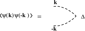
FIG. 11.: The diagram for $\langle\psi({\bf k})\psi({\bf-k})\rangle$, when $\delta=0$.

With these values substituted into (100), one can calculate

$$\langle\phi_{1}\phi_{2}\rangle \sim \langle|\psi_{1}||\psi_{2}|\rangle=\int_{-\infty}^{\infty}d\psi_{1}\int_{-\infty}^{\infty}d\psi_{2}\>|\psi_{1}||\psi_{2}|\,P[\psi_{1},\psi_{2}]$$ (104)

$$= {2C\over\pi}\left[\sqrt{1-f^{2}}+f\arctan\left(f\over\sqrt{1-f^{2}}\right)\right].$$ (105)

This correlation function can be used to find the correlation functions $\langle a_{1}a_{2}\rangle$ and $\langle a_{1}b_{2}\rangle$. Specifically

$$\langle a_{1}a_{2}\rangle={1\over 2}\langle\phi_{1}\phi_{2}+\psi_{1}\psi_{2}\rangle,$$ (106)

which gives for the connected part $\langle a_{1}a_{2}\rangle_{c}=\langle a_{1}a_{2}\rangle-\langle a\rangle^{2}$,

$$\langle a_{1}a_{2}\rangle_{c}=$$ (107)

$${\Delta\over\pi(8\pi t)^{d/2}}\left[{\pi\over 2}f-1+\sqrt{1-f^{2}}+f\arctan\left(f\over\sqrt{1-f^{2}}\right)\right]$$ (108)

For large $r$, $f=\exp(-r^{2}/8t)$ is small, giving

$$\langle a_{1}a_{2}\rangle_{c}\sim{\Delta\over 2(8\pi t)^{d/2}}e^{-r^{2}/8t}.$$ (110)

Similarly, $\langle a_{1}b_{2}\rangle=\langle\phi_{1}\phi_{2}-\psi_{1}\psi_{2}\rangle/2$, so that

$$\langle a_{1}b_{2}\rangle_{c}=$$ (111)

$${\Delta\over\pi(8\pi t)^{d/2}}\left[-{\pi\over 2}f-1+\sqrt{1-f^{2}}+f\arctan\left(f\over\sqrt{1-f^{2}}\right)\right]$$ (112)

which for large $r$ goes as

$$\langle a_{1}b_{2}\rangle_{c}\sim-{\Delta\over 4(8\pi t)^{d/2}}e^{-r^{2}/8t}.$$ (114)

A plot of these connected correlation functions is shown in Fig. 12. The signs $\langle a_{1}a_{2}\rangle>0$ and $\langle a_{1}b_{2}\rangle<0$ can be understood for short distances to be a consequence of the segregation. Given an $A$ particle at a particular point, there is an increased probability that a nearby particle is also an $A$, and a decreased probability that it is a $B$.

FIG. 12.: The correlation functions $\langle a(r,t)a(0,t)\rangle_{c}$ and $\langle a(r,t)b(0,t)\rangle_{c}$ plotted as functions of $r/\sqrt{t}$. The vertical axis is given in units of $\Delta(8\pi t)^{-d/2}$.

For the case $\delta\neq 0$ one has $\langle\psi^{2}\rangle=C(t)Q(d,\delta)$, as given by (97). The generalization of $\langle\psi({\bf k})\psi({\bf-k})\rangle$, shown in Fig. 11, behaves for small $k$ the same as when $\delta=0$. Therefore, for large $r$ one still has $\langle\psi_{1}\psi_{2}\rangle=Cf$. When this is put in the expressions for $\langle a_{1}a_{2}\rangle$ and $\langle a_{1}b_{2}\rangle$ one finds that the large $r$ behavior is given by (110) and (114) is unaffected by $\delta\neq 0$.

While these correlation functions and other quantities can be calculated, they ultimately rely on the stronger statement that $\psi$ is a gaussian random field, and that $\phi\sim|\psi|$. The topology of the domains is determined by the random field, with the boundaries between $a$ regions and $b$ regions given by the zeroes of $\psi$. This topology is completely equivalent to an analogous situation in phase ordering. It has been suggested that in the phase ordering of a scalar order parameter an invertible, non-linear mapping from the order parameter field to an auxiliary field results in the latter being a gaussian random field [23]. Usually this mapping is chosen to be the solution of a single kink, for example the hyperbolic tangent profile. While this method is no longer believed to be quantitatively correct [24], it does provide a useful picture of the structure of the domains. Again, the zeroes of this gaussian random field determine the boundaries between the equilibrated phase.

The difference between these systems lies in how correlation functions are calculated from the random field. In the reaction-diffusion case one is interested in the correlation functions of the field itself, and of the absolute value of the field. Neither of these quantities exhibit remarkable behavior. In the phase ordering one argues that at late times the mapping between the order parameter field and the gaussian field goes to a step function, and therefore order parameter correlations are given by the correlations of the sign of the random field. These sharp boundaries give rise to more interesting features, such as non-analytic terms in the small $r$ limit of the correlation function, or correspondingly power law tails for large wave number in the Fourier transform.

VI Reaction Zones

It was shown in section III A that for $d<4$ the particles segregate asymptotically into regions of purely $A$ or $B$ particles. As a result of this segregation there exist interfaces between the two species, and all reactions occur in the interfacial regions. These reaction zones have interesting scaling properties. For example, the width of the interface goes as $t^{\alpha}$ with the exponent $\alpha<1/2$. Also, the nearest neighbor distance distribution of the particles in the reaction zone is found to have a characteristic length $\ell_{\rm rz}$ that goes as a power of $t$, with an exponent which differs from that of the bulk system, where $\langle a\rangle^{-1/d}\sim t^{1/4}$. To derive these properties we begin with a related steady-state problem.

Consider a system with a source of $A$ particles located at the boundary $x=-L$ which maintains a fixed current $J\hat{\bf x}$, and a similar source $-J\hat{\bf x}$ of $B$ particles positioned at $x=L$. These opposing currents will establish a steady-state profile, in which the average densities will be functions of the transverse coordinate $x$. For a given current $J$ one can choose $L$ to be large enough that the reactions are localized to an interfacial region of width $w\ll L$. In this case, it is found that the densities in the reaction zone, where $|x|\lesssim w$, have universal scaling forms. Also of interest is the reaction rate $R(x)=\lambda_{0}\langle a(x)b(x)\rangle$, which exhibits scaling, and which is used to define the width of the reaction zone.

The power counting of section II B showed that the four-point vertices were irrelevant for $d>2$. Therefore $R(x)\sim\lambda_{\rm eff}\langle a\rangle\langle b\rangle$ in the asymptotic limit—which will be shown to be the small $J$ limit—and the problem reduces to the differential equations of the effective theory:

$${\partial\over\partial t}\langle a\rangle =\nabla^{2}\langle a\rangle-\lambda_{\rm eff}\langle a\rangle\langle b\rangle$$ (115)

$${\partial\over\partial t}\langle b\rangle =\nabla^{2}\langle b\rangle-\lambda_{\rm eff}\langle a\rangle\langle b\rangle.$$ (116)

From these equations it has been shown that

$$R\sim J^{4/3}f(xJ^{1/3}),\qquad d>2,$$ (117)

implicitly by Gálfi and Rácz [14], and later explicitly by Ben-Naim and Redner [15]. From (117) one identifies the width $w\sim J^{-1/3}$, and the characteristic length of the particle distribution within the reaction zone $\ell_{\rm rz}\equiv\langle a(x=0)\rangle^{-1/d}\sim J^{-2/3d}$. The latter quantity is derived in Ref. [16].

For $d\leq 2$ one does not have simply differential equations, and the full field theory must be taken into account. We begin by observing that the current $J_{A}$ is given by $a^{*}\partial_{x}a$ in the notation of section II B, and similarly for $J_{B}$. From dimensional analysis $[J]=k^{d+1}$.

We proceed with the renormalization of the theory, as was sketched in section III C. A normalization scale $\kappa$ is introduced, and used to define the renormalized coupling $g_{R}$. Since physical quantities, such as the width, cannot depend on $\kappa$, then

$$\kappa{d\over d\kappa}w=\left[\kappa{\partial\over\partial\kappa}+\beta(g_{R}){\partial\over\partial g_{R}}\right]w(J,g_{R},\delta,\kappa)=0.$$ (118)

Note that, since there are no diagrams which can dress the two-point vertices in (34), $\delta$ does not get renormalized, and therefore does not appear in equation above. From dimensional analysis one has

$$\left[\kappa{\partial\over\partial\kappa}+(d+1)J{\partial\over\partial J}+1\right]w(J,g_{R},\delta,\kappa)=0.$$ (119)

Combining these equations gives the Callan-Symanzik equation

$$\left[(d+1)J{\partial\over\partial J}-\beta(g_{R}){\partial\over\partial g_{R}}+1\right]w=0.$$ (120)

with the solution

$$w(J,g_{R},\delta)=\kappa J^{-1/(d+1)}w(\kappa^{d+1},\tilde{g}_{R},\delta).$$ (121)

In the small $J$ limit then $\tilde{g}_{R}\rightarrow g_{R}^{*}$, and the right-hand side is given by

$$w\sim J^{-1/(d+1)}f(\delta,\epsilon),\qquad d<2.$$ (122)

Following the same procedure for any dimensionful quantity results in the scaling behavior being given by dimensional analysis. That is, $\ell_{\rm rz}\sim w$,

$$\langle a\rangle,\langle b\rangle\sim J^{d/(d+1)}F_{a,b}(x\,J^{1/(d+1)}),$$ (123)

and

$$R(x)\sim J^{(d+2)/(d+1)}G(x\,J^{1/(d+1)}).$$ (124)

Note that these results imply that
$R\sim J^{(2-d)/(d+1)}\langle a\rangle\langle b\rangle$. This can be shown explicitly by calculating $R\propto\langle ab\rangle=\lambda(J)\langle a\rangle\langle b\rangle$, where $\lambda(J)$ is given by the bubble sum shown in Fig. 6, with $s=J^{2/(d+1)},k=0$. In the small $J$ limit then $\lambda(J)\sim J^{(2-d)/(d+1)}$.

Since the current $J$ may be thought of as being due to localized sources of $A$ and $B$ particles at $x=\pm L$ respectively, the coupling constant power counting arguments are formally the same as those of Ref. [13] (see Sec. III C), in which the sources are localized at $t=0$.[26] Thus the various scaling functions above may, in principle, be calculated as an expansion in $g_{R}^{*}=O(\epsilon)$, in which the leading term is given by the solution of the rate equations (115). The next order corrections to the reaction profile have been computed in Ref. [26], where it was shown that the fluctuation corrections lead to a universal power law tail in this function.

For $d=2$ one has $\tilde{g}_{R}\sim 1/|\ln J|$ for small $J$, and the leading order result is therefore found by substituting this behavior into the solution of the rate equation (115). This leads to the results

$$w \propto \left(|\ln J|\over J\right)^{1/3},$$ (125)

$$R(x) \sim \lambda(J)\langle a\rangle\langle b\rangle$$ (126)

$$\sim J^{4/3}|\ln J|^{-1/3}G(x\,J^{1/3}|\ln J|^{-1/3}),$$ (127)

$$\ell_{\rm rz} \propto J^{-1/3}|\ln J|^{-1/6}.$$ (128)

As was discussed in Ref. [16], the corresponding results for the time-dependent cases of segregated initial conditions or of randomly homogeneous initial conditions is given by substituting $J\propto t^{-1/2}$ or $J\propto t^{-(d+2)/4}$ (with $d=2$), respectively, in the above formulas. These results, for the case of segregated initial conditions, have been obtained recently via heuristic arguments by Krapivsky [27].

Calculation of the leading correction term for $\Delta$

In order to calculate the first order correction term to the expansion $\Delta=\Delta_{0}+\dots$ we must first comment on the bulk diagrams which generate $\lambda_{\rm eff}$. The effective coupling can be calculated as an expansion in the bare couplings, via the diagrams shown in Fig. 13. The loop integrals in this expansion require the cutoff $\Lambda$, and one finds

$$\lambda_{\rm eff}=\lambda_{2}-\lambda_{2}^{2}{4\Lambda^{d-2}\over(8\pi)^{d/2}(d-2)}+O(\lambda_{2}^{3}).$$ (129)

FIG. 13.: The expansion for the effective coupling constant. The wave number integrals are regulated by a cutoff $\Lambda$.

If the response functions in the loop of Fig. 4(c) were instead just propagators, then this set of diagrams would be included into those of Fig. 4(b) when the substitution $\lambda_{2}\rightarrow\lambda_{\rm eff}$ is made via (129). Therefore, the terms which are new and constitute a correction to $\Delta_{0}$ are those in Fig. 4(c) with the propagator loop subtracted out. We define the large $t$ limit of these diagrams to be $\Delta_{1}$, that is

$$\Delta_{1}=4\lambda_{2}^{2}n_{\phi}^{2}\int_{0}^{\infty} dt_{2}\int_{0}^{t_{2}}dt_{1}{d^{d}k\over(2\pi)^{d}}\biggl{[}{e^{-2k^{2}t}(1+n_{\phi}\lambda_{1}t_{1})^{2}\over(1+n_{\phi}\lambda_{1}t_{2})^{4}}$$ (131)

$$-{\Lambda^{d-2}\over(8\pi)^{d/2}(d-2)(1+n_{\phi}\lambda_{1}t_{2})^{2}}\biggr{]}.$$

Performing the wave number integral with the $\Lambda$ cutoff imposed in the same manner as in (129) gives $\displaystyle\Delta_{1}={4\lambda_{2}^{2}n_{\phi}^{2}\over(8\pi)^{d/2}}\int_{0}^{\infty}{dt_{2}\over(1+n_{\phi}\lambda_{1}t_{2})^{4}}$ (132) $\displaystyle\times\int_{0}^{t_{2}}dt_{1}\biggl{[}{(1+n_{\phi}\lambda_{1}t_{1})^{2}\over(t_{2}-t_{1}-\Lambda^{-2})^{d/2}}-{\Lambda^{d-2}\over d-2}(1+n_{\phi}\lambda_{1}t_{2})^{2}\biggr{]}.$ (133) The $t_{1}$ integral can be evaluated as a Laplace convolution integral, and the cutoff dependent terms cancel. The remaining $t_{2}$ integral is

$$\Delta_{1}={-8\lambda_{2}^{2}n_{\phi}^{2}\over(8\pi)^{d/2}(d-2)} \int_{0}^{\infty}{dt_{2}\>t_{2}^{1-d/2}\over(1+n_{\phi}\lambda_{1}t_{2})^{4}}$$ (135)

$$\times \biggl{[}1+{4n_{\phi}t_{2}\over 4-d}+{8n_{\phi}^{2}t_{2}^{2}\over(4-d)(6-d)}\biggr{]}.$$ (136)

This integral can be done exactly, giving

$$\Delta_{1}={\lambda_{2}^{2}\over\lambda_{1}^{2}}(n_{\phi}\lambda_{1})^{d/2}{(d+2)(d+4)\over 48(8\pi)^{d/2-1}\sin(\pi d/2)}.$$ (137)

In terms of the initial density $n_{0}$ and the effective coupling then one finds the result (6) for $\Delta$. Evaluating the diagrams such as those in Fig. 4(c), but containing more loops will then give the higher order terms in this small $n_{0}$ expansion of $\Delta$.

REFERENCES

- [1] V. Kuzovkov and E. Kotomin, Rep. Prog. Phys. 51, 1479 (1988).
- [2] A. A. Ovchinnikov, S. F. Timashev, and A. A. Belyy, Kinetics of Diffusion Controlled Chemical Processes, (Nova Science, New York, 1989).
- [3] A. A. Ovchinnikov and Ya. B. Zeldovich, Chem. Phys. 28, 215 (1978).
- [4] D. Toussaint and F. Wilczek, J. Chem. Phys. 78, 2642 (1983).
- [5] M. Bramson and J. L. Lebowitz, J. Stat. Phys. 62, 297 (1991).
- [6] M. Bramson and J. L. Lebowitz, J. Stat. Phys. 65, 941 (1991).
- [7] K. Kang and S. Redner, Phys. Rev. Lett. 52, 955 (1984).
- [8] S. Cornell, M. Droz, and B. Chopard, Physica A 188, 322 (1992).
- [9] F. Leyvraz, J. Phys. A 25, 3205 (1992).
- [10] S. Cornell and M. Droz, Phys. Rev. Lett. 70, 3824 (1993).
- [11] L. Peliti, J. Physique 46, 1469 (1985).
- [12] L. Peliti, J. Phys. A 19, L365 (1986).
- [13] B. P. Lee, J. Phys. A, 27, 2633 (1994).
- [14] L. Gálfi and Z. Racz, Phys. Rev. A 38, 3151 (1988).
- [15] E. Ben-Naim and S. Redner, J. Phys. A 25, L575 (1992).
- [16] B. P. Lee and J. Cardy, Phys. Rev. E, 50, 3287 (1994).
- [17] M. Doi, J. Phys. A 9, 1465 (1976); M. Doi, J. Phys. A 9, 1479 (1976).
- [18] L. S. Schulman, Techniques and Applications of Path Integration, (Wiley, New York, 1981) p. 242 ff.
- [19] M. Howard, private communication.
- [20] H. W. Diehl, in Phase Transitions and Critical Phenomena, edited by C. Domb and J. L. Lebowitz (Academic, New York, 1986), Vol. 10.
- [21] G. N. Watson, A Treatise on the Theory of Bessel Functions, (Cambridge, Cambridge, 1952).
- [22] see for example D. J. Amit, Field Theory, the Renormalization Group, and Critical Phenomena, (World Scientific, Singapore, 1984).
- [23] G. Mazenko, Phys. Rev. Lett. 63, 1605 (1990); G. Mazenko, Phys. Rev. B 42, 4487 (1990).
- [24] C. Yeung, Y. Oono, and A. Shinozaki, Phys. Rev. E 49, 2693 (1994).
- [25] S. Cornell, M. Droz, and B. Chopard, Phys. Rev. A 44, 4826 (1991).
- [26] M. Howard and J. Cardy, in preparation.
- [27] P. L. Krapivsky, preprint.