arch-ive/9411132

Correlation Length and Average Loop Length of the Fully-Packed Loop Model

Anton Kast

Department of Physics
University of California at Berkeley
Berkeley, California 94720, USA

The fully-packed loop model of closed paths covering the honeycomb lattice is studied through its identification with the $sl_{q}(3)$ integrable lattice model. Some known results from the Bethe ansatz solution of this model are reviewed. The free energy, correlation length, and the ensemble average loop length are given explicitly for the many-loop phase. The results are compared with the known result for the model’s surface tension. A perturbative formalism is introduced and used to verify results.

1 Review of the FPL model

In a recent article [1] Blöte and Nienhuis performed numerical investigations of what they termed the fully-packed loop (FPL) model. This is a statistical model where the ensemble is the set of all combinations of closed paths on the honeycomb lattice that visit every vertex and do not intersect. The Boltzmann weight of such a filling set of paths is just the exponential of the number of paths, i.e. the energy of a configuration is the number of closed loops used to cover the lattice. An example of a fully-packed configuration of loops on this lattice is shown in Figure 1. The partition function for this model may be represented as

$$Z_{FPL}(n)=\sum_{C}n^{P(C)}$$ (1.1)

where the sum is over all $C$, the coverings of the vertices of the hexagonal lattice by closed nonintersecting paths, $P(C)$ is the number of paths in the covering $C$, and $n$ is a generalized activity. This model was originally studied for its interest as the low-temperature limit of the $O(n)$ vector lattice models [2, 3]. In this limit, the dimensionality of vectors $n$ is just the activity $n$ in equation (1.1).

Figure 1: An example of a fully-packed loop configuration. With periodic boundary conditions, this configuration has 11 loops.

The partition function (1.1) is apparently the generating function for the numbers of ways to cover the hexagonal lattice by any number of closed paths. Its calculation in the thermodynamic limit is an interesting combinatorial problem.

More recently, Batchelor, Suzuki and Yung [4] pointed out that previous authors [5, 6] had exploited an identification of the FPL model with the integrable lattice model associated to the quantum group $sl_{q}(3)$ [7]. This integrable model is a vertex model on the square lattice where each link of the lattice can be in one of three states, and the vertex weights are given by the R-matrix for $sl_{q}(3)$ as in Figure 2. The R-matrix depends on a deformation parameter $\gamma=\log(q)$, as well as a spectral parameter $\theta$ typical of integrable theories. Denoting the $sl_{q}(3)$ partition function as $Z_{sl_{q}(3)}(\gamma,\theta)$, the precise idenfication is

$$Z_{FPL}(e^{\gamma}+e^{-\gamma})=\left.(e^{\gamma}-e^{-\gamma})^{-N}Z_{sl_{q}(3)}(\gamma,\theta)\right|_{\theta=-\gamma}$$ (1.2)

where $N$ is the volume of the lattice (the number of hexagonal faces). Since the model is integrable, much exact information can be derived. In particular, the model’s Bethe equations have been constructed and solved.

Figure 2: The definition of vertex weights in the integrable lattice model associated to $sl_{q}(d+1)$. $\gamma$ and $\theta$ are parameters of the model. States on edges are labelled by roman indices with $(d+1)$ possible values. In the formula, $\Delta_{ab}=\frac{a-b}{|a-b|}+2\frac{b-a}{d+1}$.

One of the more important results that have been derived in this way is the existence of a phase transition in the model (1.1) at $n=2$ [6, 8]. At larger $n$, larger numbers of loops are favored and at smaller $n$ configurations with fewer loops are favored. It has been conjectured that this transition is between a large-$n$ phase where the average loop length is finite and a small-$n$ phase where this average is infinite.

In section 3 a simple relation between the free energy of the FPL model and the ensemble average length of loops is derived. From the known solution to the Bethe equations of the $sl_{q}(3)$ integrable lattice model, the free energy is identified and used to graph the exact value of the average loop length as a function of $n$.

Identifying $n=e^{\gamma}+e^{-\gamma}$, it becomes apparent that $n>2$ corresponds to the integrable model for $\gamma$ real and $0<n<2$ corresponds to $\gamma$ purely imaginary. The former phase is known [7] to be massive, in the sense that there is a gap in the spectrum of eigenvalues of the transfer matrix between the leading eigenvalue and the next-leading eigenvalue. By standard arguments [10], this implies a finite correlation length. The gap tends to zero as $\gamma$ goes to zero, showing that $n=2$ is a critical point of the model (1.1).

In section 4 this correlation length is studied by considering the spectrum of eigenvalues of this transfer matrix. The spectrum may be deduced directly from the model’s Bethe equations. In the case that the transfer matrix is symmetric and therefore has real eigenvalues, the correlation length is related to the maximum eigenvalue $\Lambda_{\rm max}$ and next-leading eigenvalue $\Lambda_{1}$ by

$$\xi^{-1}=\log\frac{\Lambda_{\rm max}}{\Lambda_{1}}.$$ (1.3)

2 Review of $sl_{q}$ integrable models

The R-matrix of the $sl_{q}(d+1)$ quantum group is an $(n+1)^{2}\times(n+1)^{2}$ matrix that may be interpreted as a matrix of Boltzmann weights of a vertex model on the square lattice as shown in Figure 2. Since this matrix satisfies the Yang-Baxter equation, the associated transfer matrix commutes with itself evaluated at differing values of the spectral parameter and the model is exactly solvable by a recursive set of $d$ nested Bethe ansätze [7].

The formula for eigenvalues of the transfer matrix for the range of parameters, $\theta>-\frac{1}{2}\gamma$ and $\gamma$ real and positive, is

$$\Lambda=\prod_{k}\frac{\sinh(i\lambda_{k}+\frac{1}{2}\gamma-\theta)}{\sinh(i\lambda_{k}-\frac{1}{2}\gamma-\theta)}$$ (2.1)

where the product is over roots, $\lambda_{k}$ of a set of Bethe equations and we have neglected terms that do not contribute in the thermodynamic limit. In this limit the $\lambda_{k}$ are distributed in the interval $[-\pi/2,\pi/2]$ with the density,

$$\rho_{\rm max}(\lambda)=\sum_{m=-\infty}^{\infty}e^{2im\lambda}\frac{1}{\pi}\frac{\sinh(dm\gamma)}{\sinh[(d+1)m\gamma]}.$$ (2.2)

For eigenvalues near the maximum eigenvalue, the changes in the distribution are parameterized by the locations of holes $\theta^{q}_{h}$, $q=1\cdots d$, $h=1\cdots N_{q}$, according to

$$\rho(\lambda)-\rho_{\rm max}(\lambda)=\sum_{m=\infty}^{\infty}e^{2im\lambda}\sum_{q=1}^{d}\frac{-1}{\pi}e^{|m\gamma|}\frac{\sinh[(d+1-q)m\gamma]}{\sinh[(d+1)m\gamma]}\sum_{h=1}^{N_{q}}e^{-2im\theta^{q}_{h}}.$$ (2.3)

The numbers of holes are constrained to satisfy the relation,

$$\sum_{q=1}^{d}qN_{q}={\rm multiple\;of\;}(n+1).$$ (2.4)

The formulas (2.1), (2.3) may be combined in the thermodynamic limit to yield a formula for eigenvalues of the transfer matrix of the integrable model,

$$\log\Lambda=\int^{\pi/2}_{-\pi/2}\rho(\lambda)\log\left[\frac{\sinh(i\lambda+\frac{1}{2}\gamma-\theta)}{\sinh(i\lambda-\frac{1}{2}\gamma-\theta)}\right]\,d\lambda.$$ (2.5)

3 Free energy and average loop length

The formulas of the preceding section in the case $d=2$ yield directly the free energy density of the model (1.1) for the $n>2$ phase as the logarithm of the maximum eigenvalue of the transfer matrix, rescaled by the factor of equation (1.2). This free energy was actually derived in 1970 by Baxter [8] as the solution to a weighted three-coloring problem on the honeycomb lattice. The free energy density of the FPL model in the $n>2$ phase is

$$F_{FPL}(n) \equiv \lim_{N\rightarrow\infty}\frac{1}{N}\log Z_{FPL}(n)$$ (3.1)

$$= \log\left\{q^{1/3}\prod_{m=1}^{\infty}\frac{(1-q^{-6m+2})^{2}}{(1-q^{-6p+4})(1-q^{-6p})}\right\}$$

where $n=q+q^{-1}$, and $q=e^{\gamma}>1$. This function has an essential singularity at $q=1$. The free energy for $n<2$ and with periodic boundary conditions is given in integral form in [4].

It is interesting to note that for both phases, the free energy density gives the ensemble average length of loops. Since a configuration $C$ on a lattice of $N$ faces has $2N$ occupied links, the total length of loops is always $2N$. The average loop length of configuration $C$ is therefore $2N/P(C)$. If we define the ensemble average loop length $L_{N}(n)$ by

$$L_{N}(n)=\frac{1}{Z_{FPL}(n)}\sum_{C}\frac{2N}{P(C)}n^{P(C)},$$ (3.2)

then from inspection of equation (1.1) it is clear that

$$\frac{d}{dn}\left[L_{N}(n)Z_{FPL}(n)\right]=\frac{2N}{n}Z_{FPL}(n).$$ (3.3)

The general solution to this equation can be written up to quadrature by direct integration:

$$L_{N}(n)=\frac{1}{Z_{FPL}(n)}\int^{n}_{C}\frac{2N}{n^{\prime}}Z_{FPL}(n^{\prime})dn^{\prime}$$ (3.4)

where the lower limit of integration is an undetermined constant. In terms of the free energy density $F_{FPL}=(1/N)\log Z_{FPL}$, this becomes

$$L_{N}(n)=2Ne^{-NF_{FPL}(n)}\int^{n}_{C}\frac{e^{NF_{FPL}(n^{\prime})}}{n^{\prime}}dn^{\prime}.$$ (3.5)

The integral in equation (3.5) can be evaluated by steepest descent. The result is

$$L_{N}(n)=\frac{2N}{n}\exp\left(-Nn\frac{dF_{FPL}}{dn}(n)\right)\left[\frac{\exp\left[Nn^{\prime}\frac{dF_{FPL}}{dn}(n^{\prime})\right]}{N\frac{dF_{FPL}}{dn}(n^{\prime})}\right]^{n}_{C}.$$ (3.6)

The constant of integration may now be determined from the known value of $L_{N}(n)$ at $n\rightarrow\infty$. As will be shown in section 5, in this limit $Z_{N}(n)\simeq 3n^{N/3}$, $\frac{dF_{FPL}}{dn}(n)\simeq 1/3n$, and $L_{N}(n)=6$. These imply that $C=-\infty$, so in the thermodynamic limit

$$L_{N}(n)=\frac{2}{n\frac{dF_{FPL}}{dn}}.$$ (3.7)

In this calculation we have neglected corrections of order $1/N$ to $L_{N}(n)$.

A graph of the ensemble average loop length versus $n$ in the large-$n$ phase is shown in Figure 3. This verifies the conjecture of [6] that loop length diverges at the critical point.

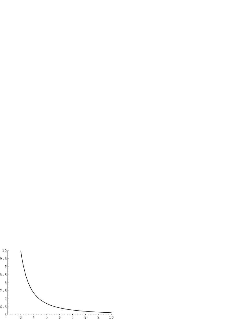
Figure 3: This is a graph of the average loop length of the FPL model versus $n$, the fugacity of loops. The critical point is at $n=2$.

4 Correlation length

To obtain the correlation length, we must compute the expression (2.5) for the minimal hole distribution. When $d=2$, there are two choices for the $N_{q}$. Either $N_{1}=3$ and $N_{2}=0$, or $N_{1}=1$ and $N_{2}=1$. In each case, the eigenvalue gap is minimized for holes at $\theta^{q}_{h}=\frac{\pi}{2}$ where the sum in equation (2.3) after integration in (2.5) is oscillatory. The transfer matrix of the model is symmetric at the point $\theta=-\frac{1}{2}\gamma$, and its eigenvalues are then real. After setting $\theta$ to this value, the correlation length of the model is given by equation (1.3).

Considering the case $N_{1}=3$ and $N_{2}=0$, we denote the next-leading eigenvalue for this hole distribution as $\Lambda_{30}$. The equation (2.5) together with the formula for densities (2.3) gives

$$\log\frac{\Lambda_{30}}{\Lambda_{\rm max}}=\sum_{m=-\infty}^{\infty}\phi_{m}\left(-\frac{1}{\pi}\right)e^{|m\gamma|}3(-1)^{m}\frac{\sinh(2m\gamma)}{\sinh(3m\gamma)}$$ (4.1)

where $\phi_{m}$ are the integrals over roots,

$$\phi_{m}\equiv\int^{\pi/2}_{-\pi/2}e^{2im\lambda}\log\left[\frac{\sinh(i\lambda+\frac{1}{2}\gamma-\theta)}{\sinh(i\lambda-\frac{1}{2}\gamma-\theta)}\right]\,d\lambda.$$ (4.2)

The integral in equation (4.2) can easily be performed by contour integration. After introducing the variables $q=e^{\gamma}$ and $z=e^{\theta}$, the result for $-\frac{1}{2}\gamma<\theta<0$ is

$$\int^{\pi/2}_{-\pi/2}e^{2im\lambda}\log\left[\frac{\sinh(i\lambda+\frac{1}{2}\gamma-\theta)}{\sinh(i\lambda-\frac{1}{2}\gamma-\theta)}\right]\,d\lambda=\left\{\begin{array}[]{ll}\frac{\pi}{m}[1-(z^{2}q^{-1})^{m}],&m>0\\ -2\pi\log z,&m=0\\ \frac{\pi}{m}[1-(z^{2}q)^{m}],&m<0\end{array}\right..$$ (4.3)

Substituting this result into equation (4.1) gives

$$\log\frac{\Lambda_{30}}{\Lambda_{\rm max}}=2\log z+3\sum_{m>0}\frac{(-1)^{m}}{m}(z^{2m}-z^{-2m})\left(\frac{q^{2m}-q^{-2m}}{q^{3m}-q^{-3m}}\right).$$ (4.4)

After expanding the demoninator of the summand in a power series in $q^{-1}$, this may be resummed to the form,

$$\log\frac{\Lambda_{30}}{\Lambda_{\rm max}}=2\log z-3\sum_{m\geq 0}\log\left[\frac{(1+z^{2}q^{-1}q^{-6m})(1+z^{-2}q^{-5}q^{-6m})}{(1+z^{-2}q^{-1}q^{-6m})(1+z^{2}q^{-5}q^{-6m})}\right].$$ (4.5)

This form is now convergent at the symmetric point, $\theta=-\frac{1}{2}\gamma$ or equivalently $z^{2}=q^{-1}$. We may therefore evaluate it there to obtain the correlation length according to equation (1.3),

$$\xi^{-1}=3\log\left\{q^{1/3}\prod_{m>0}\frac{(1+q^{2}q^{-6m})(1+q^{4}q^{-6m})}{(1+q^{-6m})(1+q^{6}q^{-6m})}\right\}$$ (4.6)

This is the desired result, the correlation length of the FPL model where $n=q+q^{-1}$ and $q>1$, or equivalently $q=+\sqrt{n^{2}-4}$.

The other possible choice of holes, $N_{1}=1$ and $N_{2}=1$ may be computed in the same way to give

$$\log\frac{\Lambda_{\rm max}}{\Lambda_{11}}=\log\left\{q\prod_{m>0}\frac{(1+q^{2}q^{-6m})(1+q^{3}q^{-6m})(1+q^{3}q^{-6m})(1+q^{4}q^{-6m})}{(1+q^{-6m})(1+qq^{-6m})(1+q^{5}q^{-6m})(1+q^{6}q^{-6m})}\right\}.$$ (4.7)

This quantity is greater than (4.6) for all $q>1$, so it is not the inverse correlation length. For large $q$, the inequality may be seen by considering the limiting forms of expressions (4.6) and (4.7). Rigorously, the multiplicands in (4.7) may be seen to be greater than those in  (4.6) term by term in $m$.

5 Perturbative analysis

The FPL model has a natural large-$n$ expansion which allows simple perturbative verifications of results.

When $n$ is large, the dominant configurations are those with large numbers of loops. The perturbative procedure is to approximate the sum over states by including the configurations with the highest numbers of loops.

On a hexagonal lattice with number of faces $N$ a multiple of three, there are three configurations with the maximum possible number of loops. In these states, one out of every three faces has a small loop around it and these small loops lie on a triangular lattice. A sample is shown in Figure 4. These three configurations differ by translations and each has $N/3$ loops.

Figure 4: A sample from a configuration with the maximum number of loops.

The smallest change in the number of loops that can be made is to introduce a defect somewhere in one of the maximal configurations, as shown in Figure 5. There are $2N/3$ different such defects that can be introduced and each reduces the number of loops by 2.

Figure 5: A configuration with two fewer than the maximum number of loops.

Introducing defects in this way, we can reach all possible configurations. To see that this is so, we can represent a configuration by labelling the links on the lattice that do not contain part of a path. One of every three links is unoccupied, and every vertex touches one unoccupied link. These unoccupied links form a dimer configuration for the vertices of the lattice. If we draw rhombuses around every dimer and interpret the resulting picture as the projection of the edges of a stack of cubes, we see that a FPL configuration is equivalent to a stack of cubes. Such an identification is shown in Figure 6.

Figure 6: An example of the identification of FPL configurations and stacks of cubes. One rhombus is drawn centered on each unoccupied link.

In this new representation, the action of inserting a defect is just the action of adding or removing a cube. This identification is exhibited in Figure 7. The result then follows that since every stack of cubes can be made by adding or removing cubes, every FPL configuration can be made from one of the maximal ones by inserting some combination of defects.

Figure 7: In the cube representation, introducing a defect is adding or removing a cube.

To obtain an approximation for the free energy, consider first the maximal state shown in Figure 4. For a lattice of $N$ faces, this configuration has $(N/3)$ loops. There are 3 such configurations corresponding to the three-fold translational degeneracy of the state. To lowest order then $Z_{FPL}=3\,n^{N/3}[1+O(n^{-1})]$. This result was used in section 3 to determine the asymptotics of the average loop length.

Allowing defects, there are $(2N/3)$ locations for a defect and each defect reduces the number of loops by two. Defects may be applied in any number and in any combination, giving the usual sum over disconnected diagrams. We can write this as the exponential of the connected diagram (one defect) and we will be correct except for the effects of excluded volumes which begin with two-defect connected diagrams and are therefore higher order. To the next order, $Z_{FPL}=3\,n^{N/3}\exp[(2N/3)n^{-2}]\exp[O(n^{-4})]$.

Perturbatively calculating the FPL free energy, we see that

$$F_{FPL}(n)=\frac{1}{3}\log(n)+\frac{2\,n^{-2}}{3}+O(n^{-4}),$$ (5.1)

in conformity with Baxter’s result shown in equation (3.1).

This point of view incidentally leads to a simple expression for the entropy density of the FPL configurations at $n=1$. At this point, all configurations are weighted equally and $Z_{FPL}$ is just the number of configurations, or the exponential of the entropy. Then calculating the partition function is just the problem of counting the number of coverings of the honeycomb lattice by paths, which is the number of different possible stacks of cubes, which is the old combinatorial problem of counting plane partitions. Elser [12] has calculated the asymptotics of plane partitions for large arrays of numbers.

The result applied to this case is entirely dependent on the shape of the boundary, even in the thermodynamic limit. This is to be expected when $n=1$, because this is in the small-$n$ phase where the model is critical. For a lattice of $N$ faces and free boundary conditions, the maximum entropy is obtained for a hexagon-shaped boundary and in that case the partition function is asymptotically

$$Z_{FPL}(1)=\exp\left[N\left(\frac{3}{2}\log 3-2\log 2\right)\right].$$ (5.2)

6 Comparison with surface tension

The ground state of the $sl_{q}(d)$ integrable lattice model is $(d+1)$-fold degenerate. This implies the existence of a notion of interfacial tension $S(\gamma)$ away from the critical point between regions of differing antiferromagnetic polarization. By considering finite-size corrections, de Vega [9] has derived transcendental equations for this interfacial tension and computed the asymptotic behavior of $S$ in the limits $\gamma\rightarrow 0$ and $\gamma\rightarrow\infty$.

Scaling arguments originally due to Widom [11] predict that the scaling relation, $S\xi\sim 1$ should hold near the critical point, $\gamma\rightarrow 0$ or equivalently $n\rightarrow 2^{+}$. It would be interesting to test this relation in this case, but we know of no explicit expression for the interfacial tension.

Away from the critical point however, a comparison can be made. The asymptotic behavior of the interfacial tension for $\gamma\rightarrow\infty$ was extracted by deVega, and the result is

$$S(\gamma)=\frac{d}{d+1}\gamma+O(1).$$ (6.1)

In the case of the FPL model, $d=2$, $n=e^{\gamma}+e^{-\gamma}$, and

$$S(n)=\frac{2}{3}\log(n)+O(1).$$ (6.2)

This result may be compared with a perturbative calculation. Consider the sum over FPL states at large-$n$ with the constraint that boundary conditions are fixed to cause frustration in the bulk, as in Figure 8. The configuration in that figure has the maximum number of loops possible and is the analog of the configuration shown in Figure 4. Denoting the sum over defects in this configuration by $Z^{\prime}_{FPL}$, the interfacial tension is defined to be the change in free energy per unit length of the interface:

$$\frac{Z^{\prime}_{FPL}}{Z_{FPL}}\sim e^{-LS}$$ (6.3)

where $L$ is the vertical size of the lattice.

Figure 8: An interface separating two regions of differing polarization.

For a lattice of N faces, the maximum number of loops possible in the presence of the constraint is $(N/3)-(2L/3)$ instead of $(N/3)$. The maximal state in the presence of the constraint is now $3\times 2^{2L/3}$-fold degenerate, because there are $(2L/3)$ locations near the interface where defects may be freely introduced without changing the number of loops. To lowest order therefore,

$$Z_{FPL} \simeq 3n^{N/3}$$ (6.4)

$$Z^{\prime}_{FPL} \simeq 32^{2L/3}n^{(N-2L)/3}.$$ (6.5)

Reading off the exponents, we have from equation (6.3) the result that

$$S(\gamma)=\frac{2}{3}\log(n)+O(1).$$ (6.6)

Equation (6.6) is apparently consistent with the large-$\gamma$ asymptotics derived in [9].

Equation (6.6) together with equation (4.6) show that $S\xi\neq 1$ in the FPL model. More generally, from the correlation length calculation it is clear that for large $\gamma$ the leading behavior of the correlation length for any value of $d$ will always be $\gamma$, and the leading behavior of $S$ is always $\gamma d/(d+1)$.

Acknowledgement

The author is grateful to Professor Nikolai Reshetikhin for many helpful conversations.

References

• [1] H.ย W.ย J.ย Blรถte, B.ย Nienhuis, Phys. Rev. Lett 72, 1372 (1994).
• [2] B.ย Nienhuis, Phys. Rev. Lett. 49, 1062 (1982).
• [3] E. Domany, D. Mukamel, B. Nienhuis, A. Schwimmer, Nucl. Phys. B190, 279 (1981).
• [4] M.ย T.ย Batchelor, J.ย Suzuki, C.ย M.ย Yung, preprint cond-mat 9408083, August 1994.
• [5] S.ย O.ย Warnaar, B.ย Nienhuis, J. Phys. A 26, 2301 (1993).
• [6] N.ย Yu.ย Reshetikhin, J. Phys. A 24, 2387 (1991).
• [7] O.ย Babelon, H.ย J.ย de Vega, C.ย M.ย Viallet, Nucl. Phys. B200 266 (1982); Nucl. Phys. B220 283 (1983).
• [8] R.ย J.ย Baxter, J. Math. Phys. 11, 784 (1970).
• [9] H.ย J.ย de Vega, J. Phys. A: Math. Gen. 20, 6023 (1987).
• [10] R.ย J.ย Baxter, Exactly Solved Models in Statistical Mechanics, New York, Academic, 1982.
• [11] B.ย Widom, J. Chem. Phys. 43, 3892 (1965).
• [12] V.ย Elser, Ph.D. Thesis, University of California, Berkeley, 1984.