Refined Simulations of the Reaction Front for Diffusion-Limited Two-Species Annihilation in One Dimension.

Abstract

Extensive simulations are performed of the diffusion-limited reaction A$+$B$\to 0$ in one dimension, with initially separated reagents. The reaction rate profile, and the probability distributions of the separation and midpoint of the nearest-neighbour pair of A and B particles, are all shown to exhibit dynamic scaling, independently of the presence of fluctuations in the initial state and of an exclusion principle in the model. The data is consistent with all lengthscales behaving as $t^{1/4}$ as $t\to\infty$. Evidence of multiscaling, found by other authors, is discussed in the light of these findings.

]

I Introduction

There has been a lot of recent interest in the scaling behaviour of the reaction front that exists between regions of initially separated reagents A and B that perform Brownian motion and annihilate upon contact according to the reaction scheme A$+$B$\to 0$[2, 3, 4, 5, 6, 7, 8, 9, 10, 11, 12, 13, 14, 15, 16, 17, 18, 19]. The evolution of the particle densities $a(x,t)$ and $b(x,t)$ at position $x$ and time $t$ is governed by the equations

$${\partial a\over\partial t} = D{\partial^{2}a\over\partial^{2}x}-R,$$ (1)

(2)

$${\partial b\over\partial t} = D{\partial^{2}b\over\partial^{2}x}-R,$$ (3)

where $R$ is the reaction rate per unit volume, and the diffusion constant $D$ has been assumed equal for both species. For the Boltzmann equation ansatz $R=kab$, the solution to the resulting partial differential equations with the initial condition

$$a(-x,0)=a_{0}\theta(x)=b(x,0),$$ (4)

where $\theta$ is the Heavyside function, has the scaling property

$$R=t^{-\alpha-(1/2)}\Phi\left({x\over t^{\alpha}}\right)\quad\hbox{ for }x\ll t^{1/2},$$ (5)

with $\alpha={1\over 6}$[2]. This result may be understood by considering the steady-state solutions to Eqs. (2) for boundary conditions $a(-x)\to J|x|/D$, $a(x)\to 0$, $b(-x)\to 0$ and $b(x)\to Jx/D$ as $x\to\infty$. Under these conditions, there are opposing constant currents $J$ of either species, and it can be shown [10, 16] that the resulting reaction profile is of the form

$$R_{ss}=J^{1+\lambda}\Phi_{ss}\left({xJ^{\lambda}}\right),$$ (6)

with $\lambda={1\over 3}$ Returning to the the time-dependent case, the quantity $(a-b)$ obeys a diffusion equation, whose solution for initial conditions (4) is

$$a-b={2a_{0}\over\sqrt{\pi}}\int_{0}^{x/(2\sqrt{Dt})}\exp\left(-{y^{2}}\right)dy.$$ (7)

Let us assume that the reaction takes place within a region of width $w\sim t^{\alpha}$, with $\alpha<{1\over 2}$. The profiles for $w\ll x\ll t^{1/2}$ are of the form $a\propto a_{0}x/t^{1/2}$, so there is a current of particles arriving the origin of the form $J=D\partial_{x}a\sim t^{-{1/2}}$. The characteristic timescale on which this current varies is $(d\log J/dt)^{-1}\propto t$, whereas the equilibration time for the front is of order $(w^{2}/D)\sim t^{2\alpha}\ll t$. The front is therefore formed quasistatically, and so Eq. (5) may be obtained from (6) simply by writing $J\propto t^{-{1/2}}$.

Simulations and experiments appear to confirm these results when the spatial dimension $d$ is two or greater[3, 4, 5, 7]. In dimension less than two, strong correlations between the motions of the two species cause the Boltzmann approximation $R=kab$ to break down. However, the solution to the steady state problem is still of the form (6), albeit with a different exponent $\lambda=1/(d+1)$[16, 18]. If the results from the steady-state may still be used, this would lead again to dynamical scaling of the form (5), with $\alpha={1\over 4}$ in $d=1$. Simulations using a one-dimensional Probabilistic Cellular Automata (PCA) model appeared to verify the dynamical scaling form (5), though with $\alpha=0.293\pm 0.005$[6]. Monte-Carlo simulations also found $\alpha\approx 0.30\pm 0.01$[9].

However, a recent article by Araujo et al [17] has challenged the validity of the scaling form (5). This article reported Monte Carlo (MC) simulations in one dimension, using an algorithm where the A and B particles always react on contact and so are unable to cross over each other. The right-most A particle (RMA) is therefore always to the left of the left-most B particle (LMB). Defining $l_{AB}$ as the separation between the RMA and LMB, and $m$ as the midpoint between them, Araujo et al found that the probability distributions $P_{l}$ and $P_{m}$ of these quantities displayed dynamic scaling, with characteristic lengthscales $t^{1/4}$ and $t^{3/8}$ respectively. Meanwhile, the different moments of the reaction profile were described by a continuous spectrum of lengthscales between $t^{1/4}$ and $t^{3/8}$. More specifically, defining

$$l^{(q)} \equiv \left(\int_{0}^{\infty}l_{AB}^{q}P_{l}(l_{AB})dl_{AB}\right)^{1/q}$$ (8)

$$m^{(q)} \equiv \left(\int_{-\infty}^{\infty}|m|^{q}P_{m}(m)dm\right)^{1/q}$$ (9)

$$x^{(q)} \equiv \left({\displaystyle\int_{-\infty}^{\infty}|x|^{q}R(x,t)dx\over\displaystyle\int_{-\infty}^{\infty}R(x,t)dx}\right)^{1/q},$$ (10)

Araujo et al found that $l^{(q)}\sim t^{1/4}$ and $m^{(q)}\sim t^{3/8}$, but $x^{(q)}\sim t^{\alpha_{q}}$ with ${1\over 4}\leq\alpha_{q}<{3\over 8}$ increasing monotonically with $q$. They also proposed the following form for $R$:

$$R(x,t)\approx t^{-{1/4}}\left({x\over t^{1/4}}\right)^{-2}\exp\left(-{|x|\over t^{3/8}}\right),$$ (11)

which predicted values of $\alpha_{q}$ that were in good agreement with their numerical findings (the prefactor $t^{-{1/4}}$, essential for consistency, is missing in [17]). The authors of [17] argued that Poisson noise in the initial state causes the reaction centre to wander anomalously as $m\propto t^{3/8}$, invalidating the use of the steady state results.

In this paper, I first describe extensive simulations of this system, using two independent models—the PCA model used in [6], and a MC model similar to that of Araujo et al in [17]. I find that dynamical scaling appears to hold for $P_{l}$, $P_{m}$, and $R$, independently of the existence of Poisson fluctuations in the initial state and of the presence of an exclusion principle. While I confirm the result $l^{(q)}\sim t^{1/4}$, I find instead that both $m^{(q)}$ and $x^{(q)}$ appear to scale as $t^{\alpha}$, with $\alpha\approx 0.28\pm 0.01$, independently of $q$. The high statistics and wide time domain accessible in the PCA simulations show that this exponent is decreasing monotonically in time, consistent with the asymptotic result $\alpha={1\over 4}$ predicted by the analogy with the steady-state result. The measured forms of $P_{l}$, $P_{m}$ and $R$ are found to be described by very simple analytic forms to high accuracy. I then discuss the validity of the fluctuation argument used by Araujo et al to explain the result $m\sim t^{3/8}$. An exact calculation of a related quantity suggests that the wandering of the reaction centre should instead be of the order $\sim t^{1/4}$, which is not sufficient to make the use of the steady-state analogy invalid. Some of these results have been discussed in a previous publication[19].

II Monte-Carlo Model

A Description of Model

The model described in Ref. [17] consists of independent random walkers with no exclusion principle. In the interests of computational efficiency, I used a model which is identical provided the site occupation number is not too large, but whose site updates may be effected using a lookup-table algorithm. In this way, it was possible to obtain statistics equivalent to the simulations in [17] in the space of a few days.

The model has an ‘exclusion principle’, in that no more than $2l_{p}$ particles of each type are allowed per site. In the diffusion step, each of these particles moves onto a neighbouring site, in such a way that no more than $l_{p}$ particles may move from a given site in the same direction at once. This constraint automatically satisfies the ‘exclusion principle’. If there are $l_{p}$ or less particles on a site, then the direction in which each particle moves is chosen independently at random. If there are more than $l_{p}$ particles, the same redistribution method is used for the ‘holes’—i.e. the probability of $j$ particles moving to the right when the occupation number is $k$ is the same as $(l_{p}-j)$ particles moving to the right when the occupation number is $(2l_{p}-k)$. The diffusion constant for this model is $1\over 2$.

In these simulations, the value $l_{p}=13$ was used (this was the largest value that could be implemented efficiently). Since the average density was 1 or less, the frequency of events where the occupation is greater than $l_{p}$ is of order $e^{-1}/(l_{p}+1)!\approx 4\times 10^{-12}$, so these events are extremely rare (the simulations represent 21000 samples of 4000 sites over 25000 timesteps, so the expected total number of such events is less than 10). The influence of such events on the results is still smaller, since the probability of a large number of particles spontaneously moving in the same direction is low (e.g. 14 independent walkers move in the same direction with probability $2^{-13}\approx 10^{-4}$). Moreover, the universality class for the scaling properties is not expected to depend on such events, as the reactions take place in the zone where the density is low. These results may therefore justifiably described as equivalent to those reported in [17]. The Fortran implementation of this algorithm performed $1.4\times 10^{7}$ site updates per second on a HP 9000/715/75 workstation.

One timestep consists of moving all the particles, followed by a reaction step. The pure diffusion algorithm has a spurious invariance, in that particles initially on even sites will always be on even sites after an even number of timesteps, and will be on odd sites at odd timesteps (and contrarily for particles initially on odd sites). In accordance with the prescription in [17] that an A particle never be found to the right of a B particle, it is important that the reaction takes account of particles of different types crossing over each other (i.e. an A-particle at site $i$ hopping to $i+1$ at the same time that a B-particle at $i+1$ hops to site $i$). The reaction algorithm first removed such particles, then annihilated any remaining A and B particles occupying the same site. This is illustrated in Fig.  1. Four sites are shown, with initially two sites occupied by A-particles (represented above the line, labeled 1–5) and two occupied by B-particles (beneath the line, labeled 6–10). In the diffusion step, each particles moves onto a neighbour at random, producing the state (ii). The reaction first deletes the A-B pair (4,6) that crossed over, leading to state (iii), then removes the pairs that sit at the same site, giving a final state (iv). If the ‘delete crossing’ step were not present, the reaction step would simply remove the pair (4,8) from state (ii), leading to a state where there are B-particles to the left of A particles.

FIG. 1.: Illustration of the Monte Carlo reaction-diffusion algorithm, showing the diffusion step and the two stages of the reaction step that first remove particles that have crossed over and then react those that are at the same site.

B Simulation Results

An approximation to a Poissonian initial state of average density unity was prepared by performing 16 attempts to add an A-particle, with probability $1/16$, to each of the first 2000 sites of a 4000-site lattice. The other half of the lattice was similarly populated with B-particles. At the boundaries, particles that attempted to leave the system were allowed to do so, but a random number (distributed binomially between 0 and 16, average $1\over 2$) of particles was allowed to re-enter the system at the end sites. The average density at the extremities was thus kept at the value unity.

In order to mimic the simulations in [17] as closely as possible, instantaneous measurements were made of $l_{AB}$, $m$, and the concentration profiles of the product and reagents at times 1000, 2500, 5000, 7500,…, 25000. These were then averaged over 21000 independent initial conditions. The quantities $l^{(q)}$ and $m^{(q)}$ were measured from the probability distributions over the samples, and a quantity $X^{(q)}$ was defined as

$$X^{(q)}=\left({\displaystyle\int x^{q}C(x,t)\,dx\over\displaystyle\int C(x,t)\,dx}\right)^{1/q},$$ (12)

where $C\equiv\int R\,dt$ is the profile of the reaction product. This quantity differs from $x{(q)}$, but since $\int C\,dx\propto t^{1/2}$, and provided that $x^{(q)}$ behaves as a power of $t$, Eq. (5) of [17] shows that they should have the same scaling behaviour.

From Eq. (2), the difference in the particle densities, $(a-b)$, obeys a simple diffusion equation, whose solution is given by (7). Any finite-size effects in the data would first show up in deviations of the particle profiles from the values they would have for an infinite system. Figure 2 shows a plot of $(a-b)$ as a function of $(x/t^{1/2})$ for three time values, displaying excellent rescaling. A simpler test of finite-size effects is to show that the total C-particle number $\Sigma_{C}\equiv\int C\,dx$ is proportional to $t^{1/2}$. The inset to Fig. 2 confirms that $\Sigma_{C}\cdot t^{-{1/2}}$ is indeed independent of time.

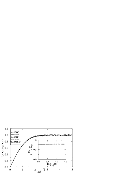
FIG. 2.: Scaling plot of the density difference $a(x,t)-b(x,t)$ for the MC data with random initial condition. Inset: bias plot for the total number of C particles $\Sigma_{C}\equiv\int C(x,t)\,dx$.

Figure 3 is a log-log plot of $X_{*}^{(q)}$, $m_{*}^{(q)}$, and $l_{*}^{(q)}$ as a function of time, where

$$X_{*}^{(q)}(t) \equiv \xi_{q}X^{(q)}(t)$$ (13)

$$m_{*}^{(q)}(t) \equiv \mu_{q}m^{(q)}(t)$$ (14)

$$l_{*}^{(q)}(t) \equiv \lambda_{q}l^{(q)}(t),$$ (15)

and $\xi_{q}$, $\mu_{q}$, and $\lambda_{q}$ are constants that will be defined later. The straight lines are fits to the last 8 points for $X_{*}^{(2)}$, $m_{*}^{(2)}$, and $l_{*}^{(1)}$. The gradients for least squares fits to the curves in Fig. 3 are listed in Table I. The exponent describing $l^{(q)}$ is close to $\frac{1}{4}$, as was found in [17]. However, the results for $m^{(2)}$ and $X^{(2)}$ differ dramatically from those of Araujo et al. Firstly, the exponent describing $m(t)$ appears to be close to $0.29$, instead of 0.375 as they found. Secondly, the exponents describing $X^{(q)}$ appear to be independent of $q$. This means that $C(x,t)$, and by implication $R(x,t)$, obeys a simple scaling form, in contrast to the anomalous form (11).

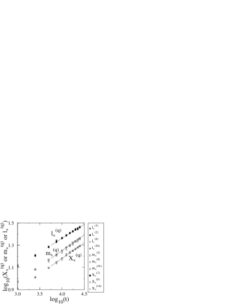
FIG. 3.: Log-log plot of $l_{*}^{(q)}$, $m_{*}^{(q)}$, and $X_{*}^{(q)}$ (see text) from the MC simulations with Poisson initial conditions.

To investigate for a trend in the exponents describing these quantities, the effective exponent (defined as the gradient between successive points in Fig. 3) is plotted as a function of $1/\log_{10}(t)$ in Fig. 4. The data for $l^{(1)}$ and $m^{(2)}$ are far too noisy for any information to be obtained. The exponent for $X^{(2)}$ appears to to decrease slowly in time, but the time window in these simulations is too narrow for conclusive deductions to be made.

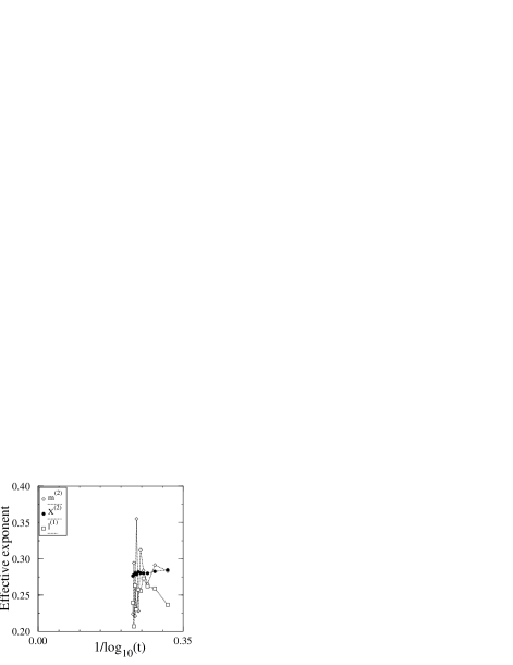
FIG. 4.: Effective exponents for $l^{(1)}$, $m^{(2)}$, and $X^{(2)}$ (see text) from the MC simulations.

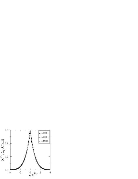
FIG. 5.: Scaling plot for $C(x,t)$, for the MC simulations.

Figures 5, 6, and 7 are plots of $C$, $P_{m}(m)$ and $P_{l}(l_{AB})$, as a function of appropriate scaling variables, to show the subjective quality of scaling for these quantities. The profiles of $P_{m}(m)$ and $P_{l}(l_{AB})$ suggest the following forms:

$$P_{m}(m) = {1\over m_{0}\sqrt{\pi}}\exp\left[-\left({m\over m_{0}}\right)^{2}\right]$$ (16)

$$P_{l}(l) = {2l\over l_{0}^{2}}\exp\left[-\left({l\over l_{0}}\right)^{2}\right]$$ (17)

These forms predict the following results for the moments of these distributions:

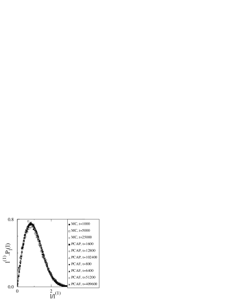
FIG. 6.: Scaling plot for $P_{l}(l)$, for the MC simulations (‘MC’) and the PCA simulations with Poisson (‘PCAP’) and full (‘PCAF’) initial conditions.

$$m^{(q)}=\mu_{q}^{-1}m_{0},\qquad l^{(q)}=\lambda_{q}^{-1}l_{0},$$ (18)

where

$$\mu_{q} = \left({(q/2)!\over q!}\right)^{1/q}\left[1+(-1)^{q}\right],$$ (19)

$$\lambda_{q} = \cases{\mu_{q+1}(\sqrt{\pi}/2)^{1/q}&for $q$ odd,\cr\left[(q/2)!\right]^{1/q}&for $q$ even.}$$ (20)

Using these values of $\mu_{q}$ and $\lambda_{q}$ in Eqs. (13–15), one would expect $m_{*}^{(q)}$ and $l_{*}^{(q)}$ to be independent of $q$ if the forms (16,17) are valid. The coincidence of the curves in Fig. 3 confirms this.

Figure 8 is an explicit test of the forms (16,17) against the data, by plotting $\log[m^{(2)}P_{m}(m)]$ and $\log[l^{(2)}l^{-1}P_{l}(l)]$ against $(m/m^{(2)})^{2}$ and $(l/l^{(2)})^{2}$ respectively, at $t=25000$. The Y-ordinate has been shifted so that all curves are coincident at the origin. The curve labeled $R_{\rm MC}$ is $\log[C(x,25000)-C(x,22500)]$, which is approximately proportional to $R(x,25000)$, as a function of $(x/X^{(2)})^{2}$. The straight line for this curve suggests that the reaction profile $R(x,t)$ is also a Gaussian. This again contradicts the form (11) proposed by Araujo et al. It is not possible, however, to derive analytical forms for $\xi_{q}$ that lead to $X_{*}^{(q)}$ being independent of $q$ without assuming a form for $x^{(q)}(t)$ for all $t$, so the values of $\xi_{q}$ used in Eq. (13) were chosen numerically in an ad hoc fashion.

III Probabilistic Cellular Automata Model

A Description of Model

This model has been described extensively in previous publications[6, 20]. In the one-dimensional realization of this model, there are up to two particles of each species at each site, labeled by the direction from which they moved onto the site at the previous timestep. The diffusion step consists of changing the velocities of these particles, then moving the particles onto the neighbouring sites according to their new velocities. If there are two particles per site, they both move in opposite directions, whereas a single particle will change direction with probability $p$. The value used in these simulations was $p=\frac{1}{2}$, so that the particle forgets its previous velocity at each timestep, and the model is equivalent to the MC model with $l_{p}=1$.

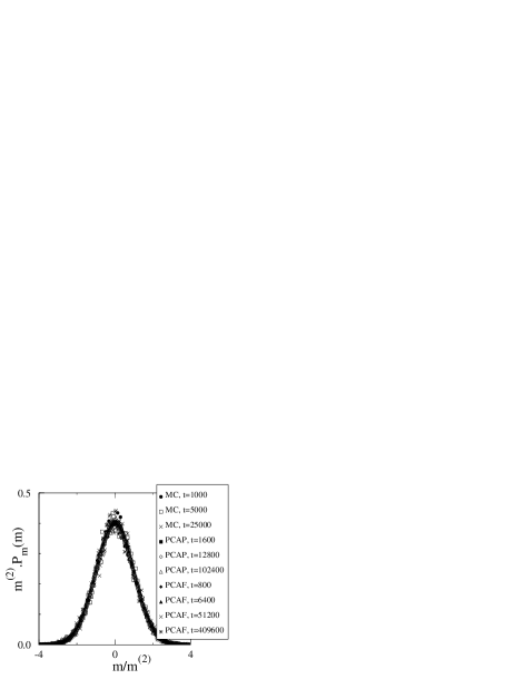
FIG. 7.: Scaling plot for $P_{m}(m)$, for the MC simulations (‘MC’) and the PCA simulations with Poisson (‘PCAP’) and full (‘PCAF’) initial conditions.

The reaction step consists of checking each site for simultaneous occupancy of A and B particles at the start of the timestep , and removing any pairs that hopped onto the site from opposite directions. Using the segregated initial condition, and this ‘infinite’ reaction rate, a site can only be occupied by an A-B pair if the A arrived from the left and the B from the right. This model has the same two-sublattice structure as the Monte-Carlo model defined above, and this is preserved by the reaction algorithm, so these two sublattices must be viewed as two independent systems. There is therefore an independent nearest-neighbour A-B pair for each sublattice. A multi-spin-coding implementation of the algorithm simulates 64 independent systems at once.

The quantities $P_{m}(m)$, $P_{l}(l)$ and $R(x,t)$ at measurement time $t$ were estimated by averaging over the interval $t(1-\delta)<t<t(1+\delta)$, with $\delta=0.05$. We may estimate the order of magnitude of the systematic error that this introduces into the measured shape of these quantities. Let $\tilde{F}(x,t)$ be the estimate of a function $F(x,t)$ using the above method. Then

$$\tilde{F} \equiv \frac{1}{2t\delta}\int_{t(1-\delta)}^{t(1+\delta)}F(x,t^{\prime})\,dt^{\prime}$$ (21)

$$= \frac{1}{2t\delta}\int_{t(1-\delta)}^{t(1+\delta)}\left(F(x,t)+(t^{\prime}-t)\frac{\partial}{\partial t}F(x,t)\right.$$ (23)

$$\phantom{\frac{1}{2\delta t}\int_{t(1-\delta)}^{t(1+\delta)}\Bigl{(}}\left.+{1\over 2}(t^{\prime}-t)^{2}\frac{\partial^{2}}{\partial t^{2}}F(x,t)+\dots\right)dt^{\prime}$$

$$= F(x,t)+\frac{(t\delta)^{2}}{6}\frac{\partial^{2}}{\partial t^{2}}F(x,t)+{\cal O}\left[(t\delta)^{4}\right].$$ (24)

The fractional error is therefore of order $(t\delta)^{2}\ddot{F}/(6F)$.

FIG. 8.: Fits of $P_{m}$, $P_{l}$, and $R$ to Eqs. (16), (17) and (28) from the MC simulations (‘MC’) and PCA simulations with Poisson (‘PCAP’) and full (‘PCAF’) initial conditions. X-axis rescaled and Y-axis shifted for clarity. For curve ‘$R_{MC}$’, see text.

This systematic error has no effect on the scaling behaviour, however. If $F(x,t)=t^{b}\phi(x/t^{a})$, we have

$$\tilde{F}(x,t) = \frac{1}{2t\delta}\int_{t(1-\delta)}^{t(1+\delta)}(t^{\prime})^{b}\phi\left(\frac{x}{(t^{\prime})^{a}}\right)dt^{\prime}$$ (25)

$$= t^{b}\tilde{\phi}\left({x\over t^{a}}\right),$$ (26)

where $\tilde{\phi}(y)\equiv(2\delta)^{-1}\int_{1-\delta}^{1+\delta}\theta^{b}\phi(y\theta^{-a})d\theta$, so $\tilde{F}$ has the same scaling properties as $F$.

In order to maximize the statistics, the reaction profile $R$ was measured at every timestep between $t(1-\delta)$ and $t(1+\delta)$. However, the quantities $m$ and $l$ are much more cumbersome to measure using this program (due to the multi-spin coding), and so were only measured every 10 timesteps. No significant loss in statistics is incurred, since these quantities have very strong time autocorrelations. The Fortran implementation of this algorithm performed $3.7\times 10^{7}$ site updates per second on a HP 9000/715/75 workstation.

B Simulation Results

1 Poisson Initial Condition

An initial condition with Poisson-like density fluctuations was prepared by filling each of the appropriate site variables (A particle for $x<0$, B particles for $x>0$) with probability ${1\over 4}$. The lattice size was 4000 sites, and at the boundaries particles were free to leave the system, with the density at the boundary maintained at an average value of $1\over 2$ by allowing A particles to enter from the left, and B particles to enter from the right, randomly with probability $1\over 4$. Measurements were taken at times 200-102400 timesteps, with the interval between measurements doubling progressively. The quantities $P_{m}(m)$, $P_{m}(l)$ and $R(x,t)$ were measured as described above, and then averaged over 82176 independent realizations of the system. The quantities $m^{(q)}$, $l^{(q)}$ and $x^{(q)}$ were then measured from the $(1/q)$’th power of the normalized $q$’th moment of these quantities.

Figure 9 shows a plot of $(a-b)$ as a function of $(x/t^{1/2})$ for three time values, and a plot of $\Sigma_{R}\cdot t^{1/2}$ (where $\Sigma_{R}\equiv\int R\,dx$) as a function of $t$. These plots show that, just as in the MC simulations, there are no finite size effects.

Figure 11 is a log-log plot of $x_{*}^{(q)}$, $m_{*}^{(q)}$ and $l_{*}^{(q)}$ as a function of time, where

$$x_{*}^{(q)}\equiv\mu_{q}x^{(q)},$$ (27)

and $\mu_{q}$ is the appropriate scaling factor for Gaussian distributions (see Eqs.  (14) and (19)). The curves for $m_{*}^{(q)}$ have been shifted vertically (by 0.2) for clarity, otherwise they would be too close to the curves for $x_{*}^{(q)}$. The straight lines are a fit to the last 5 points, for the lowest values of $q$. The gradients of least-square fits for all the curves are summarized in Table I. The collapse of the curves for different values of $q$ confirms both the scaling hypothesis and the forms for the scaling functions (16,17), and also that the reaction rate profile has a Gaussian form:

$$R(x,t)={\Sigma_{R}\over w\sqrt{\pi}}\exp\left[-\left({x\over w}\right)^{2}\right].$$ (28)

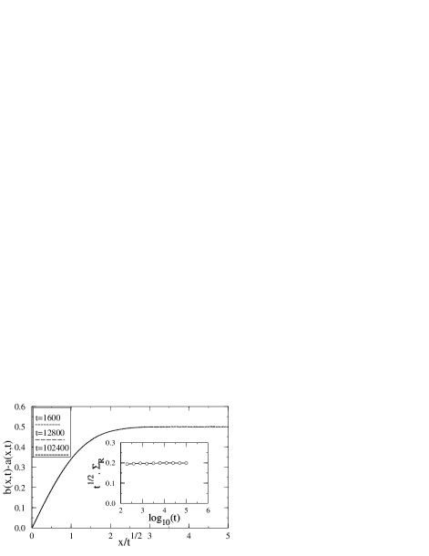
FIG. 9.: Scaling plot of the density difference $a(x,t)$ $-b(x,t)$ for the PCA data with random initial condition. Inset: bias plot for the total reaction rate $\Sigma_{R}\equiv\int R\,dx$.

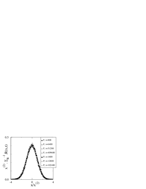
FIG. 10.: Scaling plot for $R(x,t)$, for the PCA simulations with Poisson (‘P’) and full (‘F’) initial conditions.

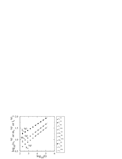
FIG. 11.: Log-log plot of $l_{*}^{(q)}$, $m_{*}^{(q)}$, and $x_{*}^{(q)}$ (see text) from the PCA simulations with Poisson initial conditions. The curves for $m^{(q)}$ has been shifted vertically for clarity.

Figure 12 shows the effective exponents for $x^{(2)}$, $m^{(2)}$ and $l^{(1)}$, from the successive gradients in Fig. 11. The curves are much less noisy than those in Fig. 4, by virtue of higher statistics and the use of coarse-grained time averages. There is a clear trend for the effective exponent for $x^{(2)}$ to decrease as time increases, consistent with the asymptotic value ${1\over 4}$ predicted elsewhere [16, 18]. The exponent for $m^{(2)}$ appears to increase initially, but the last few points appear also to decrease, and in any case an asymptotic value $0.375$ is ruled out.

The rescaled forms of $P_{l}(l)$, $P_{m}(m)$, and $R$ are denoted by ‘PCAP’ in Figs. 6, 7, and 10 respectively. Figure 8 shows a fit of $P_{l}(l)$, $P_{m}(m)$ and $R$ to the forms (16,17,28). From Eq. (21), using $F(x,t)=At^{-\beta}\exp(-\lambda x^{2}/t^{\alpha})$, the fractional error introduced by the coarse-grained time averaging is found to be $\approx(\delta^{2}/6)(x/w)^{4}$, where $w^{2}=(\int x^{2}F\,dx/\int F\,dx)$. The measurement of these quantities is therefore expected to be accurate for the first four decades or so, as is indeed observed.

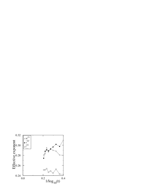
FIG. 12.: Effective exponents for $l^{(1)}$, $m^{(2)}$, and $x^{(2)}$ (see text) from the PCA simulations with Poisson initial conditions.

2 Full Initial Conditions

Because of the exclusion principle in the PCA model, the system is completely static in regions where the occupation number is zero for one species and assumes its maximal value for the other. If one starts from a lattice that is filled with A-particles up to $x=0$, and filled with B-particles for $x>0$, simulations may be speeded up by only updating the lattice in the region where a ‘hole’ has penetrated. By checking explicitly that such holes never reach the physical boundary of the system, it is possible to perform simulations on a system that is effectively infinite, so having no finite-size effects.

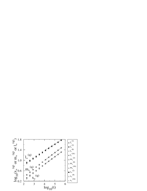
FIG. 13.: Log-log plot of $l_{*}^{(q)}$, $m_{*}^{(q)}$, and $x_{*}^{(q)}$ (see text) from the PCA simulations with full initial conditions. The curves for $m^{(q)}$ has been shifted vertically for clarity.

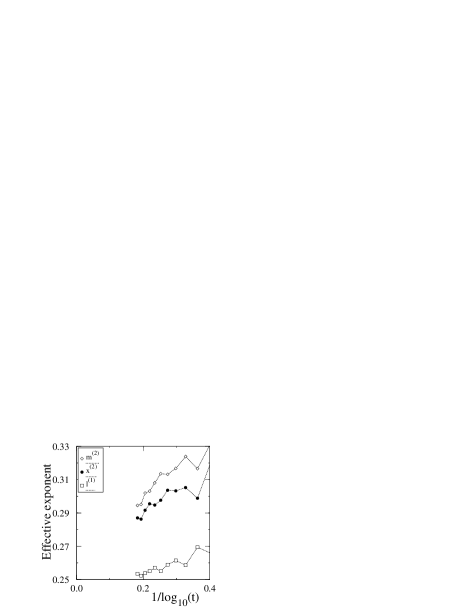
FIG. 14.: Effective exponents for $l^{(1)}$, $m^{(2)}$, and $x^{(2)}$ (see text) from the PCA simulations with full initial conditions.

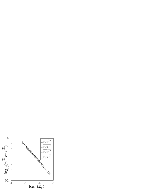
FIG. 15.: Plot of $x^{(2)}$ and $m^{(2)}$ against the time-dependent current for the two sets of PCA simulations.

Simulations of 64000 independent evolutions of a full lattice were run for 409600 timesteps. Measurements of $P_{m}(m)$, $P_{l}(l)$, and $R$ were made using the same method as for the Poisson initial condition. Results for these simulations are shown in Figs. 13 and 14. It might be expected (considering the arguments in [17]) that this case would be in a different universality class from the case with randomness in the initial state. However, the results for the exponents (see Table I) are very close to those measured for the case of Poisson initial conditions, and the marked decrease of the exponents for $x^{(2)}$(arguably towards $0.25$) is also seen in Fig. 14. It is interesting to note that the transient trends in $m^{(2)}$ and $l^{(1)}$ are in the opposite sense to the Poisson case.

Scaling plots for $P_{l}$, $P_{m}$ and $R$ are shown in Figs. 6, 7, and 10, denoted by ‘PCAF’. Plots of $l^{-1}P_{l}$, $P_{m}$, and $R$ may be found in Fig. 8, confirming that the profiles again have the forms (16,17,28).

Figure 15 is a plot of $m^{(2)}$ and $x^{(2)}$ as a function of the time dependent current $\Sigma_{R}=\int R\,dx$, from the simulations both with (‘P’) and without (‘F’) Poisson fluctuations in the initial state. The two curves for $x^{(2)}$ are almost coincident, which is what would be expected if the reaction profile depended upon the current only. The curves for $m^{(2)}$, however, are not quite coincident, showing that this quantity is more sensitive to the initial condition. Incidentally, numerical tests showed that the diffusion current at the origin has Poissonian noise whether the initial state contained such fluctuations or not.

IV The Effect of Poissonian Fluctuations in the Initial State

The measured value $m\sim t^{3/8}$ in Ref. [17] was justified by an argument about the Poisson fluctuations in the initial condition. The argument went as follows: after time $t$, particles within a distance $\sim t^{1/2}$ have had a chance of participating in the reaction. The number of particles within a distance $t^{1/2}$ is of order $t^{1/2}\pm ct^{1/4}$. Since each reaction event kills precisely one A and one B, there is therefore a local surplus $\sim t^{1/4}$ of one of the species. The majority species therefore invades the minority species by a distance $m$, such that the number of minority particles between the origin and $m$ is $\sim t^{1/4}$. Since the particle profiles vary like $x/t^{1/2}$, this means that $\int_{0}^{m}(x/t^{1/2})dx\sim t^{1/4}$, so $m\sim t^{3/8}$

In order to assess the validity of this argument, it is possible to apply it to a related quantity upon which analytical calculations may be made. Consider the diffusion equation $\partial_{t}\rho(x,t)={1\over 4}\partial_{x}^{2}\rho(x,t)$ in one spatial dimension, with an initial condition that consists of a random series of negative Dirac delta peaks for $x<0$ and positive Dirac delta peaks for $x>0$. That is,

$$\rho(x,t=0)=\sum_{i=1}^{\infty}\delta(x-x_{i})-\sum_{i=1}^{\infty}\delta(x+y_{i}),$$ (29)

where $x_{i}>0$, $y_{i}>0$. If the intervals between the $x_{i}$ and $y_{i}$ have a Poisson distribution, one has

$$\langle\rho(x,0)\rangle = \hbox{sign}(x),$$ (30)

$$\langle\rho(x,0)\rho(y,0)\rangle = \hbox{sign}(xy)+\delta(x-y),$$ (31)

where $\langle\rangle$ represents an average over the variables $x_{i}$, $y_{i}$.

The solution for $\rho$ may be written in the form

$$\rho(x,t) = \int_{-\infty}^{\infty}\rho(x^{\prime},0)(\pi t)^{-{1/2}}\exp\left({-{(x-x^{\prime})^{2}\over t}}\right)dx^{\prime}$$ (32)

$$= \sum_{i}(\pi t)^{-{1/2}}\left[\exp\left({-{(x-x_{i})^{2}\over t}}\right)\right.$$ (34)

$$\phantom{\sum_{i}(\pi t)^{-{1/2}}\left[\right.}\left.-\exp\left({-{(x+y_{i})^{2}\over t}}\right)\right].$$

Consider the gradient of $\rho$:

$$\partial_{x}\rho = \sum_{i}2(\pi t)^{-{1/2}}\left[{x-x_{i}\over t}\exp\left({-{(x-x_{i})^{2}\over t}}\right)\right.$$ (36)

$$\phantom{\sum_{i}2(\pi t)^{-{1/2}}\left[\right.}\left.-{x+y_{i}\over t}\exp\left({-{(x+y_{i})^{2}\over t}}\right)\right]$$

$$= 2{x\over t}\rho(x,t)$$ (39)

$$+\sum_{i}(\pi t^{3})^{-{1/2}}\left[x_{i}\exp\left({-{(x-x_{i})^{2}\over t}}\right)\right.$$

$$\phantom{+\sum_{i}(\pi t^{3})^{-{1/2}}\left[\right.}\left.+y_{i}\exp\left({-{(x+y_{i})^{2}\over t}}\right)\right].$$

The second term on the right hand side of Eq. (39) is strictly positive. The gradient of $\rho$ when $\rho$ is zero is therefore strictly positive, so, since $\rho$ is continuous for all $t>0$, $\rho$ is zero at precisely one point, $x_{0}(t)$ (say).

It is possible to find the probability distribution of these zeros, $P(x_{0})$, over the ensemble of initial states. The position $x_{0}$ is defined by $\rho(x_{0},t)=0$, or, equivalently,

$$\int_{-\infty}^{\infty}\rho(z,0)\exp\left({-{z^{2}\over t}}\right)\exp\left({-{2zx_{0}\over t}}\right)dz=0.$$ (40)

Suppose that $x_{0}\sim t^{a}$, where $a$ is expected to be less that ${1\over 2}$, and let $\epsilon=t^{b+(1/2)}$, with $0<b<({1\over 2}-a)$. Then the contribution to the integral in (40) for $|x|>\epsilon$ is of order $\exp(-\epsilon^{2}/t)\sim\exp(-t^{2b})$, which vanishes as $t\to\infty$. However, for $|x|<\epsilon,$ the argument of the second exponential has upper bound $2\epsilon x_{0}/t\to 0$, and so the asymptotic value of the integral is found by using the first few terms only of the Taylor expansion of this exponential. In other words, the leading contribution to $x_{0}$ as $t\to\infty$ is given by

$$\int_{-\infty}^{\infty}\rho(z,0)e^{-{z^{2}\over t}}dz-{2x_{0}\over t}\int_{-\infty}^{\infty}\rho(z,0)z\,e^{-{z^{2}\over t}}dz=0.$$ (41)

The expectation value of the second moment of $x_{0}$ is

$$\langle x_{0}^{2}\rangle={t^{2}\over 4}\left\langle{\int\rho(x,0)e^{-{x^{2}\over t}}dx\over\int x\rho(x,0)e^{-{x^{2}\over t}}dx}{\int\rho(y,0)e^{-{y^{2}\over t}}dy\over\int y\rho(y,0)e^{-{y^{2}\over t}}dy}\right\rangle$$ (42)

To evaluate this average, write $\rho(x,0)=\hbox{sign}(x)+\tau(x)$, where $\langle\tau(x)\rangle=0$ and $\langle\tau(x)\tau(y)\rangle=\delta(x-y)$. Then $\int x\rho(x,0)\exp({-{x^{2}/t}})dx=t+\int x\tau(x)\exp({-{x^{2}/t}})dx$, the second term being typically much smaller than the first. To find the leading contribution to $x_{0}$, it is sufficient to replace $\int x\rho(x,0)\exp({-{x^{2}/t}})dx$ in the denominator by $t$. We therefore have

$$\langle x_{0}^{2}\rangle = {1\over 4}\int_{-\infty}^{\infty}\int_{-\infty}^{\infty}\langle\rho(x,0)\rho(y,0)\rangle$$ (44)

$$\phantom{{t\over 4}\int_{-\infty}^{\infty}\int_{-\infty}^{\infty}\langle}\times\exp\left({-{x^{2}+y^{2}\over t}}\right)dxdy+\dots$$

$$= {1\over 4}\int_{-\infty}^{\infty}e^{-{2x^{2}\over t}}dx+\dots$$ (45)

$$= {1\over 2}\sqrt{\pi t\over 8}+\dots$$ (46)

Similarly, the $2n$’th moment of $P(x_{0})$ is of the form

$$\langle x_{0}^{2n}\rangle = {1\over 2^{2n}}\int_{-\infty}^{\infty}dx_{1}\dots\int_{-\infty}^{\infty}dx_{2n}$$ (50)

$$\phantom{{t\over 2}^{n}\int_{-\infty}^{\infty}}\times\exp\left(-{\sum_{i=1}^{2n}x_{i}^{2}\over t}\right)$$

$$\phantom{{t\over 2}^{n}\int_{-\infty}^{\infty}\times}\times\langle\rho(x_{1},0)\dots\rho(x_{2n},0)\rangle+\dots$$

$$= {(2n)!\over 2^{2n}n!}\left({\pi t\over 8}\right)^{n/2}+\dots$$ (51)

For a distribution of the form $P(x_{0})=\sqrt{(\lambda/\pi)}\exp(-\lambda x_{0}^{2})$, one has

$$\langle x_{0}^{2n}\rangle={(2n)!\over 2^{2n}\lambda^{n}n!}.$$ (52)

Comparison with (51) gives

$$P(x_{0})={2\over\pi}\sqrt{2\over t}\exp\left(-\sqrt{8\over\pi t}x_{0}^{2}\right).$$ (53)

The distribution of $x_{0}$ is therefore characterized by a single lengthscale $\lambda^{-{1/2}}\propto t^{1/4}$.

Figure 16 shows the moments of $P_{0}$, averaged over 10000 realizations, from a numerical solution of the zero of $\rho$ from Eq.  (34), compared with the asymptotic predictions of Eq.  (51).

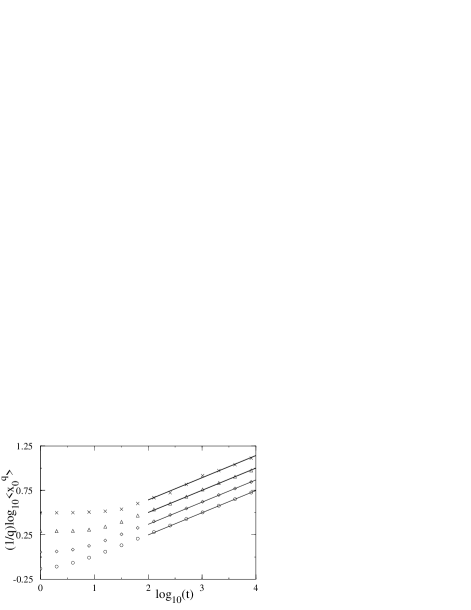
FIG. 16.: Log-log plot of $\langle x_{0}^{q}\rangle$ versus $t$ for $q=2$ ($\circ$), 4 ($\diamond$), 8 ($\triangle$) and 16 ($\times$), from numerical solutions of Eq. (34). The straight lines are the asymptotic solutions from Eq.  (51).

From Eq. (2), the density difference $(a-b)$ in the reaction-diffusion problem, averaged over evolutions, obeys a simple diffusion equation. The quantity $\rho$ with the initial condition (29) is therefore equal to $(a-b)$ for the initial condition with Poisson fluctuations used in the numerical simulations, with negative peaks corresponding to A particles and positive peaks corresponding to B particles. The quantity $x_{0}$ differs from $m(t)$ because the latter contains further fluctuations due to the diffusive noise that has been averaged over in the former. However, the argument used in [17] to obtain $m\sim t^{3/8}$ may be applied equally well to $x_{0}$. The reaction centre shifts to compensate for a local majority of order $t^{1/4}$ in one of the species, and the argument predicts $x_{0}\sim t^{3/8}$. It is interesting to note that the correct exponent is obtained if the initial value $a(x,0)=a_{0}$ is used instead of the value $a(x,t)\propto{x/t^{1/2}}$ at time $t$ in the balance equation $\int^{x_{0}}a(x,t)\sim t^{1/4}$. This ambiguity is probably the reason for the argument being incorrect.

TABLE I.: Comparison of the simulation results in this paper for the Monte-Carlo model (MC) and PCA model with Poisson (PCAP) and Full (PCAF) initial conditions with those of Araujo et al (ALHS)[17]. Numbers in parentheses represent the statistical error in the preceding digit.

	ALHS	MC	PCAP	PCAF
Size	2000	4000	4000	Infinite
Exclusion prle.?	No	Noa	Yes	Yes
Initial density	1.0	1.0	0.5	2.0
Initial State	(Uniform)	Poisson	Poisson	Uniform
Averaging	6000–15000	21000	82176	64000
Max time	25000	25000	102400	409600
Exponents:
$l^{(1)}$	0.25	0.251(3)	0.2510(6)	0.2542(4)
$l^{(16)}$	0.25	0.23(1)	0.248(3)	0.2609(3)
$m^{(2)}$	0.375	0.281(4)	0.287(1)	0.300(1)
$m^{(16)}$	0.375	0.29(1)	0.284(1)	0.299(3)
$x^{(2)}$	0.312	0.2799(2)b	0.286(2)	0.291(1)
$x^{(8)}$	0.359	0.282(2)b	0.280(4)	0.293(1)
$x^{(16)}$	0.367	0.30(2)b	0.28(1)	0.293(2)
Fit over last…	N/A	8 points	5 points	6 points

V Conclusions

It appears from extensive simulations that the reaction profile in this system has the same simple dynamic scaling form, independently of the presence of an exclusion principle and of randomness in the initial state. The motion of the reaction centre due to the Poisson noise appears only to account for a contribution of order $\sim t^{1/4}$ to the reaction width, which is not large enough to alter the scaling behaviour. The measured exponent $\approx 0.29$ describing both the reaction width and the midpoint fluctuations appears in fact to be decreasing slowly in time, with favourable evidence for an asymptotic value $0.25$. This, together with the measured form for the reaction profile, is consistent with the steady-state results being applicable[16, 18, 21].

It is, nevertheless, surprising that the approach to the asymptotic behaviour should be so slow. It is not clear whether logarithmic corrections should be present, as they do not occur in the steady-state problem[18]. However, in these simulations the ratio of the reaction width $w$ to the diffusion length $(Dt)^{1/2}$ was never smaller than $\approx 0.2$, whereas the application of the steady-state argument requires that this ratio be small. This could account for the fact that the asymptotic regime has not been reached. Simulations where this ratio is truly small would not appear to be practical at present.

An investigation of the simulation procedure used by Araujo et al has revealed a few errors in the results published in [17]. A repeat of their simulations appears to confirm the results of the present article for $P_{m}$ and $P_{l}$, and the behaviour $m\sim t^{0.30}$, but does not find that $R$ satisfies a scaling ansatz[22]. This inconsistency between my results and those of Araujo et al is currently unexplained.

A recent calculation by Rodriguez and Wio[23] suggests that the reaction profile $R$ should be the superposition of two scaling forms, with width exponents ${1\over 3}$ and ${3\over 8}$ respectively. However, these exponents and the form they predict for $R$ ($\sim\exp[-(x/w)^{3/2}]$) do not agree with the results of simulations. The approximation scheme they used would therefore not appear to be valid, unless it describes a regime inaccessible to simulations.

The simulation evidence in favour of dynamic scaling in this model is very strong. However, the numerical evidence that all lengthscales scale asymptotically as $t^{1/4}$ is far from conclusive, and so needs to be put on a sound theoretical basis, either by an exact calculation or by a rigorous justification for the analogy with the static case.

REFERENCES

- [1] Address from January 1995: Department of Physics, University of Guelph, Guelph, Ontario N1G 2W1, Canada.
- [2] L. Gálfi and Z. Rácz, Phys. Rev. A 38, 3151 (1988).
- [3] Y.-E. Koo, L. Li, and R. Kopelman, Mol. Cryst. Liq. Cryst. 183, 187 (1990).
- [4] Z. Jiang and C. Ebner, Phys. Rev. A 42, 7483 (1990).
- [5] B. Chopard and M. Droz, Europhys. Lett. 15 459 (1991).
- [6] S. Cornell, M. Droz, B. Chopard, Phys. Rev. A 44, 4826 (1991).
- [7] Y.-E. Koo and R. Kopelman, J. Stat. Phys. 65, 893 (1991).
- [8] H. Taitelbaum, S. Havlin, J. Kiefer, B. Trus, and G. Weiss, J. Stat. Phys 65, 873 (1991).
- [9] M. Araujo, S. Havlin, H. Larralde, H.E. Stanley, Phys. Rev. Lett. 68 1791 (1992).
- [10] E. Ben-Naim and S. Redner, J. Phys. A 25, L575 (1992)
- [11] H. Larralde, M. Araujo, S. Havlin, and H. E. Stanley, Phys. Rev. A 46, 855 (1992).
- [12] H. Larralde, M. Araujo, S. Havlin, and H. E. Stanley, Phys. Rev. A 46 6121 (1992).
- [13] S. Cornell, M. Droz, B. Chopard, Physica A188, 322 (1992).
- [14] H. Taitelbaum, Y.-E. Koo, S. Havlin, R. Kopelman, and G. Weiss, Phys Rev. A 46, 2151 (1992).
- [15] B. Chopard, M. Droz, T. Karapiperis, and Z. Racz, Phys. Rev. E 47, 40 (1993).
- [16] S. Cornell and M. Droz, Phys. Rev. Lett. 70, 3824 (1993).
- [17] M. Araujo, H. Larralde, S. Havlin, and H.E. Stanley, Phys. Rev. Lett. 71 3592 (1993).
- [18] B. Lee and J. Cardy, Phys. Rev. E, to appear (1994).
- [19] S. Cornell, Phys. Rev. Lett. to appear (1994).
- [20] B. Chopard and M. Droz, J. Stat. Phys. 64, 859 (1991).
- [21] S. Cornell and M. Droz, in preparation (1994).
- [22] M. Araujo, private communication.
- [23] Rodriguez and Wio, preprint, (1994).