Andreev reflection in ferromagnet–superconductor junctions

Abstract

The transport properties of a ferromagnet–superconductor (FS) junction are studied in a scattering formulation. Andreev reflection at the FS interface is strongly affected by the exchange interaction in the ferromagnet. The conductance $G_{\text{FS}}$ of a ballistic point contact between F and S can be both larger or smaller than the value $G_{\text{FN}}$ with the superconductor in the normal state, depending on the ratio of the exchange and Fermi energies. If the ferromagnet contains a tunnel barrier (I), the conductance $G_{\text{FIFS}}$ exhibits resonances which do not vanish in linear response — in contrast to the Tomasch oscillations for non-ferromagnetic materials.

Electrons in a metal can not penetrate into a superconductor if their excitation energy with respect to the Fermi level is below the superconducting gap $\Delta$. Still, a current may flow through a normal-metal–superconductor (NS) junction in response to a small applied voltage $V<\Delta/e$, by means of a scattering process known as Andreev reflection and64 : An electron in the normal metal is retroreflected at the NS interface as a hole and a Cooper pair is carried away in the superconductor. Andreev reflection near the Fermi level conserves energy and momentum but does not conserve spin — in the sense that the incoming electron and the Andreev reflected hole occupy opposite spin bands. This is irrelevant for materials with spin-rotation symmetry, as is the case for normal metals. However, the change in spin band associated with Andreev reflection may cause an anomaly in the conductance of (metallic) ferromagnet–superconductor (FS) junctions, because the spin-up and the spin-down band in the ferromagnet are different. This paper contains a theoretical study of Andreev reflection in FS junctions. We use a scattering approach based on the Bogoliubov-de Gennes equation to study the transport properties for zero temperature and small $V$ ($eV\ll\Delta$). We will concentrate on two distinct effects, which we think are experimentally observable. First, due to the change in spin band there is no complete Andreev reflection at the FS interface. This has a clear influence on the conductance and the shot-noise power of clean FS point contacts. Second, the different spin-up and spin-down wavevector at the Fermi level may lead to quantum-interference effects. This shows up in the linear-response conductance of FIFS junctions, where the ferromagnet contains an insulating tunnel barrier (I).

In the past, FS junctions with an insulating layer between the ferromagnet and the superconductor have been used in spin-dependent tunneling experiments mes94 . There the emphasis was on the voltage scale $eV\gtrsim\Delta$ and Andreev reflection did not play a role. Tunneling through S–Fi–S junctions, where Fi is a magnetic insulator, has been studied both experimentally sta85 and theoretically dew85 ; kup91 . In addition, there has been theoretical work on the Josephson effect in SFS junctions bul82 ; kup86 . An experimental investigation of the boundary resistance of sputtered SFS sandwiches has also been reported fie90 . The importance of phase coherence was demonstrated in a recent experiment pet94 , in which the effect of a remote superconducting island on the conductance of a ferromagnet was observed. We do not know of any previous theoretical work on the influence of Andreev reflection on the sub-gap conductance of an FS junction.

In order to clarify the effects we are aiming at, let us first give an intuitive and simple description of the conductance through a ballistic FS point contact. A ferromagnet is contacted through a small area with a superconductor. The transverse dimensions of the contact area are much smaller than the mean free path and the interface is clean, so that the conductance is completely determined by the scattering processes that are intrinsic to the FS interface. In a semiclassical approximation all scattering channels (transverse modes in the point contact at the Fermi level) are fully transmitted, when the superconductor is in the normal state. Let $N_{\uparrow}(N_{\downarrow})$ be the number of up(down)-spin channels, so that $N_{\uparrow}\geq N_{\downarrow}$. At zero temperature, the spin channels do not mix and the conductance is given by the Landauer formula

$$G_{\text{FN}}=\frac{e^{2}}{h}\,(N_{\downarrow}+N_{\uparrow})\>.$$ (1)

In the superconducting state, the spin-down electrons of all the $N_{\downarrow}$ channels are Andreev reflected into spin-up holes. They give a double contribution to the conductance since $2e$ is transferred at each Andreev reflection. However, only a fraction $N_{\downarrow}/N_{\uparrow}$ of the $N_{\uparrow}$ channels can be Andreev reflected, because the density of states in the spin-down band is smaller than in the spin-up band. Therefore, the resulting conductance is

$$G_{\text{FS}}=\frac{e^{2}}{h}(2N_{\downarrow}+2\frac{N_{\downarrow}}{N_{\uparrow}}N_{\uparrow})=4\,\frac{e^{2}}{h}\,N_{\downarrow}\>.$$ (2)

Comparison of Eqs. (1) and (2) shows that $G_{\text{FS}}$ may be either larger or smaller than $G_{\text{FN}}$ depending on the ratio $N_{\uparrow}/N_{\downarrow}$. If $N_{\downarrow}/N_{\uparrow}<1/3$ then $G_{\text{FS}}<G_{\text{FN}}$, and vice versa. This qualitative argument can be substantiated by an explicit calculation, as we now show.

For the conduction electrons inside the ferromagnet we apply the Stoner model, using an effective one-electron Hamiltonian with an exchange interaction. The effect of the ferromagnet on the superconductor is twofold. First, there is the influence of the exchange interaction on states near the interface. This will be fully taken into account. Second, there is the effect of the magnetic field due to the magnetization of the ferromagnet. Since this field — which is typically a factor thousand smaller than the exchange field — does not break spin-rotation symmetry it will be neglected for simplicity. Note that in typical layered structures the magnetization is parallel to the FS interface, so that it has no influence on the superconductor at all.

Transport through NS junctions has successfully been investigated through the Bogoliubov-de Gennes equation btk82 ; lam91 ; tak92 ; bee92 . Here, we adopt this approach for an FS junction. In the absence of spin-flip scattering in the ferromagnet, the Bogoliubov-de Gennes equation breaks up into two independent matrix equations, one for the up-electron, down-hole quasiparticle wavefunction $(u_{\uparrow},v_{\downarrow})$ and another one for $(u_{\downarrow},v_{\uparrow})$. Each matrix equation has the form SM&A

$$\left(\begin{array}[]{cc}{\cal H}_{0}-h&\Delta\\ \Delta^{*}&-({\cal H}_{0}+h)\end{array}\right)\left(\begin{array}[]{c}u_{\uparrow}\\ v_{\downarrow}\end{array}\right)=\varepsilon\left(\begin{array}[]{c}u_{\uparrow}\\ v_{\downarrow}\end{array}\right)\>.$$ (3)

Here, $\varepsilon$ is the quasiparticle energy measured from the Fermi energy $E_{F}\equiv\hbar^{2}k_{F}^{2}/2m$, ${\cal H}_{0}\equiv{\bf p}^{2}/2m+V-E_{F}$ is the single-particle Hamiltonian, with $V({\bf r})$ the potential energy, $h({\bf r})$ is the exchange energy, and $\Delta({\bf r})$ is the pair potential. For simplicity, it is assumed that the ferromagnet and the superconductor have identical ${\cal H}_{0}$. For comparison with experiment, our model can easily be extended to include differences in effective mass and band bottom. We adopt the usual step-function model for the pair potential btk82 ; lam91 ; tak92 ; bee92 and do the same for the exchange energy bul82 ; kup86 . Defining the FS interface at $x=0$ with S at $x>0$, we have $\Delta({\bf r})=\Delta\Theta(x)$ and $h({\bf r})=h_{0}\Theta(-x)$, with $\Theta(x)$ the unit step-function.

A scattering formula for the linear-response conductance of an NS junction is given by Takane and Ebisawa tak92 . Application to the FS case is straightforward,

$$G_{\text{FS}}=2\,\frac{e^{2}}{h}\sum\limits_{\sigma=\uparrow,\downarrow}\mbox{Tr}\,{\bf r}_{h\bar{\sigma},e\sigma}^{\dagger}{\bf r}_{h\bar{\sigma},e\sigma}^{\vphantom{\dagger}}\>,$$ (4)

where the matrix ${\bf r}_{h\bar{\sigma},e\sigma}$ contains the reflection amplitudes from incoming electron modes with spin $\sigma$ to outgoing hole modes with spin $\bar{\sigma}$ (opposite to $\sigma$) evaluated at the Fermi level ($\varepsilon=0$). We first consider a ballistic point contact. We assume that the dimensions of the contact are much greater than the Fermi wavelength, as is appropriate for a metal, so that quantization effects can be neglected. The number $N_{\downarrow}$ of minority spin modes in the point contact (with area $\Omega$) is $N_{\downarrow}=N_{0}(1-h_{0}/E_{F})$, with $N_{0}\equiv k_{F}^{2}\Omega/4\pi$ the number of modes per spin for a non-ferromagnetic ($h_{0}=0$) contact of equal area. The reflection matrices for this case can be evaluated by matching the bulk solutions for the ferromagnet and for the superconductor at the interface. An incoming electron from the ferromagnet is either normally reflected as an electron of the same spin or Andreev reflected as a hole with the opposite spin. (Transmission into the superconductor is not possible at $\varepsilon=0$.) The reflection matrices are diagonal, with elements

$$r_{ee} \equiv r_{e\sigma,e\sigma}=r_{h\sigma,h\sigma}=\frac{k_{\uparrow}k_{\downarrow}-q^{2}}{k_{\uparrow}k_{\downarrow}+q^{2}}\>,$$ (5a)

$$r_{he} \equiv r_{h\bar{\sigma},e\sigma}=r_{e\bar{\sigma},h\sigma}=\frac{-2iq\sqrt{k_{\uparrow}k_{\downarrow}}}{k_{\uparrow}k_{\downarrow}+q^{2}}\>,$$ (5b)

where the longitudinal wavevectors $k_{\uparrow(\downarrow)}$ in the ferromagnet and $q$ in the superconductor are defined in terms of the energy $E_{n}$ of the $n$-th transverse mode by

$$q = \sqrt{(2m/\hbar^{2})(E_{F}-E_{n})}\>,$$ (6a)

$$k_{\uparrow} = \sqrt{(2m/\hbar^{2})(E_{F}-E_{n}+h_{0})}\>,$$ (6b)

$$k_{\downarrow} = \sqrt{(2m/\hbar^{2})(E_{F}-E_{n}-h_{0})}\>.$$ (6c)

In the above expressions terms of order $\Delta/E_{F}$ are neglected notAA . Note that $|r_{ee}|^{2}+|r_{he}|^{2}=1$, as required from quasiparticle conservation. It follows from Eq. (5) that a clean FS junction does not exhibit complete Andreev reflection, in contrast to the NS case. This is due to the potential step the particle passes when being Andreev reflected to the opposite spin band.

Because of the large number of modes the trace in Eq. (4) can be replaced by an integration, which can be evaluated analytically. The result is

$$G_{\text{FS}} = 4\,\frac{e^{2}}{h}\,N_{0}\,\frac{4}{15\eta^{4}}\,\times$$ (7)

$$[\sqrt{1-\eta^{2}}(6-7\eta^{2}+\eta^{4})-6+10\eta^{2}-4\eta^{5}]\>,$$

where $\eta\equiv h_{0}/E_{F}$. The conductance is plotted in Fig. 1, and compared with the semiclassical estimate from Eq. (2), which turns out to be quite accurate. Since $N_{\uparrow}+N_{\downarrow}=2N_{0}$ one has from Eq. (1) $G_{\text{FN}}>G_{\text{FS}}$ if $h_{0}>0.47E_{F}$, or equivalently $N_{\downarrow}/N_{\uparrow}<0.36$.

Further information on the Andreev reflection at the FS interface can be obtained from the shot-noise power $P$ of the junction. Shot noise is the time-dependent fluctuation in the current due to the discreteness of the charges. For uncorrelated electron transmission, one has the maximal noise power of a Poisson process $P_{\text{Poisson}}\equiv 2eI$, with $I$ the mean current. On the one hand, correlations due to the Pauli principle reduce $P$ below $P_{\text{Poisson}}$ khl87 ; les89 . On the other hand, Cooper-pair transport across an NS junction has been shown to manifest itself as a doubling of the maximal noise power khl87 ; jon94 . We apply the general result of Ref. jon94 to the FS junction

$$P_{\text{FS}}=\frac{8e^{3}V}{h}\sum\limits_{\sigma=\uparrow,\downarrow}\mbox{Tr}\,{\bf r}_{h\bar{\sigma},e\sigma}^{\dagger}{\bf r}_{h\bar{\sigma},e\sigma}^{\vphantom{\dagger}}({\bf 1}-{\bf r}_{h\bar{\sigma},e\sigma}^{\dagger}{\bf r}_{h\bar{\sigma},e\sigma}^{\vphantom{\dagger}})\>.$$ (8)

Substitution of Eq. (5b) into Eq. (8) yields the shot-noise power of a ballistic point contact, plotted in Fig. 1. The shot noise increases from complete suppression for a non-ferromagnetic ($h_{0}=0$) junction to twice the Poisson noise for a half-metallic ferromagnet ($h_{0}=E_{F}$). The initial increase is slow, indicating that the $N_{\downarrow}$ modes undergo nearly complete Andreev reflection. However, for higher exchange energies the Andreev reflection probability decreases in favour of the normal reflection probability. This is manifested by the increase in the shot-noise power.

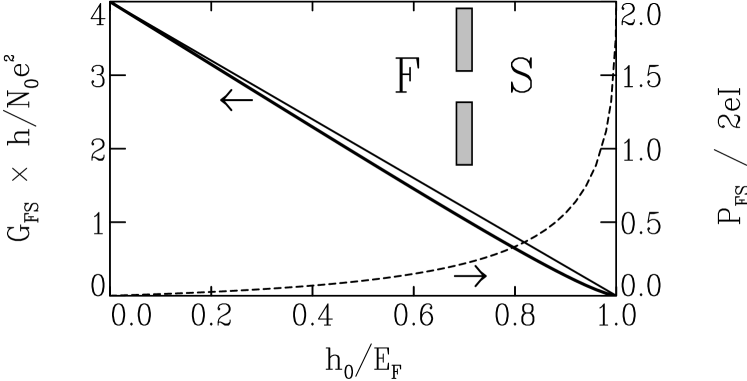
Figure 1: The conductance $G_{\text{FS}}$ (full curves) and the shot-noise power $P_{\text{FS}}$ (dashed) of a ballistic point contact in a ferromagnet–superconductor junction (see inset), as a function of the exchange energy $h_{0}$. The thick line represents the exact result (7) for $G_{\text{FS}}$, the thin line the estimation (2).

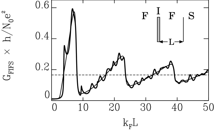
Figure 2: The conductance $G_{\text{FIFS}}$ of a clean FIFS junction containing a planar tunnel barrier (transparency $\Gamma$) on the ferromagnetic side, as a function of the separation $L$ from the interface (see inset). The thick solid line is computed from Eq. (9) for $\Gamma=0.1$, $h_{0}=0.2E_{F}$. For the thin line normal reflection at the FS interface is neglected ($r_{ee}=0$). The dashed line is the classical large-$L$ limit.

Figure 3: Numerical calculation of the effect of disorder in the ferromagnet on the oscillations shown in Fig. 2 for a clean junction. The disordered region is modeled by a $L\times W$ square lattice (lattice constant $a$) with random on-site disorder (uniformly distributed between $\pm U/2$). The width $W=101a$ is fixed and the length $L$ is varied on the horizontal axis. The results shown are for $E_{F}=\hbar^{2}/2ma^{2}$, $h_{0}=0.2E_{F}$, $\Gamma=0.1$, and for various $U$. For each disorder strength $U$ the bulk mean free path $\ell$ is given. Thick lines belong to one realization of disorder, thin to an average over 20 realizations.

The second system we consider is an FIFS junction which contains a planar tunnel barrier (I) at $x=-L$. The barrier is modeled by a channel- and spin-independent transmission probability $\Gamma\in[0,1]$. The matrix ${\bf r}_{h\bar{\sigma},e\sigma}^{\dagger}{\bf r}_{h\bar{\sigma},e\sigma}^{\vphantom{\dagger}}$ in Eq. (4) is diagonal, with elements

$$|r_{h\bar{\sigma},e\sigma}|^{2}=\Gamma^{2}\,|r_{he}|^{2} \Bigl{\{} 1+2\rho^{2}\cos(\chi_{\uparrow}-\chi_{\downarrow})+\rho^{4}$$ (9)

$$+ 2r_{ee}\rho(1+\rho^{2})(\cos\chi_{\uparrow}+\cos\chi_{\downarrow})$$

$$+ 2r_{ee}^{2}\rho^{2}[1+\cos(\chi_{\uparrow}+\chi_{\downarrow})]\,\Bigl{\}}^{-1}\,,$$

where $\rho\equiv\sqrt{1-\Gamma}$ and $\chi_{\sigma}\equiv 2k_{\sigma}L$. Eq. (9) describes resonant Andreev reflection: Due to the different wavevector of up electrons and down holes, $|r_{h\bar{\sigma},e\sigma}|^{2}$ varies as a function of $\chi_{\uparrow}$ and $\chi_{\downarrow}$ between $\Gamma^{2}$, the value for a two-particle tunneling process, and 1 for full resonance. The conductance $G_{\text{FIFS}}$ is evaluated by substitution of Eq. (9) into Eq. (4). It is depicted in Fig. 2 as a function of $L$ for $h_{0}=0.2E_{\text{F}}$ and $\Gamma=0.1$. The resonances have a dominant period $\delta L=\pi\hbar v_{F}/2h_{0}(=5\pi k_{F}^{-1}$ in Fig. 2), which is caused by the simplest round-trip containing two Andreev reflections and two barrier reflections. Superimposed one sees oscillations with smaller period, caused by longer trajectories in which also normal reflections at the FS interface occur. This becomes clear when we calculate $G_{\text{FS}}$ with $r_{ee}$ set to zero, which is also shown in Fig. 2. For large $L$, $G_{\text{FIFS}}$ approaches the classical (i.e. all interferences are neglected) value $4(e^{2}/h)N_{\downarrow}\Gamma/(2-\Gamma)$. The oscillations in Fig. 2 are distinct from the Tomasch oscillations known to occur in the non-linear differential conductance of NINS junctions tom65 . There, quasi-bound states arise because electron and hole wavevectors disperse if $\varepsilon>0$. However, in linear response $G_{\text{NINS}}=4(e^{2}/h)N_{0}\Gamma^{2}/(2-\Gamma)^{2}$, independent of $L$ btk82 . In the ferromagnetic junction the resonances do not vanish in linear response, in contrast to the Tomasch oscillations. The quasi-bound states at the Fermi level are a direct consequence of the change in spin band upon Andreev reflection.

We believe that both phenomena are experimentally accessible. The FS point contact can be constructed according to the nanofabrication technique of Ref. hol91 . The FIFS junction can be made by growing a wedge-shaped layer of ferromagnet on a superconducting substrate and then depositing a thin oxide layer. This allows a measurement of $G_{\text{FIFS}}$ for different values of $L$. It is not necessary for the contact area to be small, so that no nanofabrication techniques are needed. (Note, that in order to observe the resonances due to the quasi-bound states it is not essential that the contact on top of the barrier is a ferromagnet.) To estimate the effect of disorder (growth imperfections and impurities) on the resonances, we have numerically calculated $G_{\text{FIFS}}$ for a disordered ferromagnet between the barrier and the FS interface. The computations are similar to the NS case treated in Ref. mar93 . The disordered region is modeled by a tight-binding Hamiltonian on a square lattice with a random impurity potential at each site. (For computational efficiency the geometry is two-dimensional, but this makes no qualitative difference.) The matrix ${\bf r}_{h\bar{\sigma},e\sigma}$ is obtained by combining the scattering matrix of the disordered region with the reflection coefficients for the FS interface (5). We then calculate $G_{\text{FS}}$ through Eq. (4). The result for various disorder strengths is shown in Fig. 3. For the clean case we recognize a behavior similar to Fig. 2. Adding some disorder removes the small-period oscillations but preserves the dominant oscillations. Only quite a strong disorder (for the top curve $k_{F}$ $\times$ bulk mean free path $\simeq$ 9) is able to smooth away the resonances.

In summary, we have shown that the transport properties of ferromagnet–superconductor junctions are qualitatively different from the non-ferromagnetic case, because the Andreev reflection is modified by the exchange interaction in the ferromagnet. Two illustrative examples have been given: For a ballistic FS point contact it is found that the conductance can be both larger or smaller than the normal-state value and for an FIFS junction containing a tunnel barrier conductance resonances are predicted to occur in linear response.

We are especially grateful to H. van Houten for suggesting the problem treated in this paper. Furthermore, we thank P. J. Kelly and C. M. Schep for useful discussions. This research was supported by the Dutch Science Foundation NWO/FOM.

References

- (1) A. F. Andreev, Zh. Eksp. Teor. Fiz. 46, 1823 (1964) [Sov. Phys. JETP 19, 1228 (1964)].
- (2) A recent review is: R. Meservey and P. M. Tedrow, Phys. Rep. 238, 173 (1994).
- (3) F. Stageberg, R. Cantor, A. M. Goldman, and G. B. Arnold, Phys. Rev. B32, 3292 (1985).
- (4) M. J. DeWeert and G. B. Arnold, Phys. Rev. Lett. 55, 1522 (1985); Phys. Rev. B 39, 11307 (1989).
- (5) S. V. Kuplevakhskiĭ and I. I. Fal’ko, Fiz. Met. Metalloved. 71, 68 (1991) [Phys. Met. Metallogr. 71, 65 (1991)].
- (6) L. N. Bulaevskiĭ, A. I. Buzdin, and S. V. Panjukov, Solid State Commun. 44, 539 (1982).
- (7) S. V. Kuplevakhskiĭ and I. I. Fal’ko, Fiz. Met. Metalloved. 62, 13 (1986) [Phys. Met. Metallogr. 62, 8 (1986)]; Pis’ma Zh. Eksp. Teor. Fiz. 52, 957 (1990) [JETP Lett. 52, 340 (1990)].
- (8) C. Fierz, S.-F. Lee, J. Bass, W. P. Pratt, Jr., and P. A. Schroeder, J. Phys. Condens. Matter 2, 9701 (1990).
- (9) V. T. Petrashov, V. N. Antonov, S. V. Maksimov, and R. Sh. Shaĭkhaĭdarov, Pis’ma Zh. Eksp. Teor. Fiz. 59, 523 (1994) [JETP Lett. 59, 551 (1994)].
- (10) G. E. Blonder, M. Tinkham, and T. M. Klapwijk, Phys. Rev. B 25, 4515 (1982).
- (11) C. J. Lambert, J. Phys. Condens. Matter 3, 6579 (1991).
- (12) Y. Takane and H. Ebisawa, J. Phys. Soc. Jpn. 61, 1685 (1992).
- (13) C. W. J. Beenakker, Phys. Rev. B 46, 12841 (1992).
- (14) P. G. de Gennes, Superconductivity of Metals and Alloys (Benjamin, New York, 1966).
- (15) This is the Andreev approximation and64 . One can easily go beyond it by including terms of order in Eqs. (5) and (6). We have checked that this has only a small influence on our final results. In fact, the larger , the more accurate is the Andreev approximation.
- (16) V. A. Khlus, Zh. Eksp. Teor. Fiz. 93, 2179 (1987) [Sov. Phys. JETP 66, 1243 (1987)].
- (17) G. B. Lesovik, Pis’ma Zh. Eksp. Teor. Fiz. 49, 513 (1989) [JETP Lett. 49, 592 (1989)]; M. Büttiker, Phys. Rev. Lett. 65, 2901 (1990).
- (18) M. J. M. de Jong and C. W. J. Beenakker, Phys. Rev. B49, 16070 (1994).
- (19) W. J. Tomasch, Phys. Rev. Lett. 15, 672 (1965); 16, 16 (1966); W. L. McMillan and P. W. Anderson, Phys. Rev. Lett. 16, 85 (1966); A. Hahn, Phys. Rev. B31, 2816 (1985).
- (20) P. A. M. Holweg, J. A. Kokkedee, J. Caro, A. H. Verbruggen, S. Radelaar, A. G. M. Jansen, and P. Wyder, Phys. Rev. Lett. 67, 2549 (1991).
- (21) I. K. Marmorkos, C. W. J. Beenakker, and R. A. Jalabert, Phys. Rev. B48, 2811 (1993).