Density waves and $1/f$ density fluctuations in granular flow

Abstract

We simulate the granular flow in a narrow pipe with a lattice–gas automaton model. We find that the density in the system is characterized by two features. One is that spontaneous density waves propagate through the system with well–defined shapes and velocities. The other is that density waves are so distributed to make the power spectra of density fluctuations as $1/f^{\alpha}$ noise. Three important parameters make these features observable and they are energy dissipation, average density and the rougness of the pipe walls.

PACS numbers: 05.20.Dd, 47.50.+d, 47.20.-k, 46.10.+z

I. INTRODUCTION

Granular materials, like powders or beads, are widely processed in industry. In this kind of materials, many unusual phenomena such as size segregation [1, 2, 3, 4], heap formation and convection cells under vibration [5, 6, 7, 8], and anomalous sound propagation [9, 10] have been found. Even in simple geometries like hoppers and pipes, their flow under gravity still shows complex dynamics [11, 12, 13]. Experiments [11, 12, 13] and molecular dynamics (MD) simulations [13, 14, 15] show that the granular particles do not flow uniformly but rather form density waves (or shock waves). The density fluctuation in the granular flow was observed to follow a $1/f^{\alpha}$ noise both in experiments [11, 12, 16] and in MD simulations [14].

We have studied the granular flow through a narrow pipe using a lattice–gas automaton (LGA). Since a general theory for granular media is not yet available, people have used various methods to get better understanding about the complicated rheological behavior of granular media. Among the different methods are MD [2, 14, 17, 18], Monte Carlo simulations [4, 19], event driven algorithms [20] and cellular automaton [21]. So far the most widely used method is MD [22] which simulates the granular materials on a “microscopic” level (the grain’s level). MD has been recognized to be very successful in simulating granular materials. MD needs, however, much computer time to give reasonable results. The same situation was also faced in classical fluid mechanics some years ago when Frisch, Hasslacher and Pomeau [23] proposed lattice–gas automata as an alternative to the direct solution of the equation of motion. The basic idea behind LGA is that a properly defined cellular automaton with appropriate conservation laws should lead to the Navier–Stokes equation which is nothing but an expression of the conservation of momentum. Guided by this spirit we have designed an LGA for granular flow. Some of our results have been briefly reported in Ref. [24]. In the present paper we will give a detailed account of our results obtained with this model. The paper is organized as follows. We describe the model in the following section and present the numerical results in section III. A discussion is contained in section IV.

II. THE LGA MODEL

We consider an LGA at integer time steps $t=0,1,2,\cdots$ with $N$ particles located at the sites of a two–dimensional triangular lattice which is $L$ sites long vertically and $W$ sites wide horizontally. Gravity is parallel to one of the lattice axes. Periodic boundary conditions are used in the vertical direction while fixed boundary conditions are set for the walls. At each site there are seven Boolean states which refer to the velocities, $\vec{v}_{i}(i=0,1,2,\cdots 6)$. Here $\vec{v}_{i}(i=1,2,\cdots 6)$ are the nearest neighboring (NN) lattice vectors and $\vec{v}_{0}=\vec{0}$ refers to the rest (zero velocity) state. Each state can be either empty or occupied by a single particle. Therefore, the number of particles per site has a maximal value of $7$ and a minimal value of 0. The time evolution of the LGA consists of a collision step and a propagation step. In the collision step particles change their velocities due to collisions and in the subsequent propagation step particles move in the directions of their velocities to the NN sites where they collide again.

The system is updated in parallel. Only the specified collisions shown in figure 1 can deviate the trajectories of particles. All collisions conserve mass and momentum.

For two– and three–body collisions, we have the probabilistic rules shown in figure 1 (a). The probablity that a configuration may take place is shown next to the configuration. If the parameter $p$ is nonzero, it means that energy can be dissipated in the collision.

The collision rules for moving particles with a rest particle involve typical mechanisms of granular flow. Intuitively one can understand them as follows. Rest particles in a region will decrease the local granular temperature which is defined as the (kinetic) energy, causing a decrease in pressure in that region. The resulting pressure gradient will lead to a migration of particles into that region, increasing its density and decreasing its pressure and granular temperature even more [25, 26]. That means that rest particles will effectively attract rest particles nearby. However, due to the restriction of LGA that the rest state at one site can at most be occupied by one particle, we must introduce some additional constraints in our model. For example, two moving particles colliding with a rest particle from opposite directions can stop each other in accordance with momentum conservation. But on each site only one rest particle is allowed. Therefore, the two particles stay at rest on the NN sites where they originally came from. However, on these sites there may already exist other rest particles. To make things simple, we will still use the on–site collision as defined and temporarily allow more than one rest particle on a site during the collision. Immediately after the collision, the extra rest particles randomly hop to NN sites until they find a suitable site with no rest particle already sitting there. Only in this way can we incorporate the mechanisms mentioned above. The collision rules with rest particles are shown in figure 1 (b).

The driving force of the flow is gravity. We simply incorporate its effect as follows. A rest particle decides to have a velocity along the direction of gravity with probability $g$, if the resulting state is empty at that time. Any moving particle can change its velocity by a unit vector along gravity with probability $g$, if the resulting state is possible on the trianglar lattice used. These are depicted in figure 1 (c).

The sites at the walls of the system only have two directions into which the particles can move. So, a particle colliding with the wall from one direction can be bounced back with probability $b$ and specularly reflected into the other direction with probability $1-b$. If $b=0$, the walls are smooth (perfect no–slip condition). Otherwise, the walls have some roughness. The collision rule is depicted in figure 1 (d).

III. RESULTS
A. Density Contrast

We evolve the system according to the collision rules defined above. The initial configuration of the system is set to be random in the sense that every state (except the rest state) of each site is randomly occupied according to a preassigned average density $\rho$. Figure 2 shows the time evolution of the density in the pipe during the early stage for $p=0.1,g=0.5,b=0.5$. Here the system has length $L=2200$ and width $W=11$ with average density $\rho=1.0$ (note the range of $\rho$ is between $0$ and $7$). We divided the pipe along the vertical direction into $220$ bins with equal length of $10$ (total length $L=2200$) and counted the number of particles $n_{i}$ in the $i$th bin, i. e., within an area $W\times 10$. Therefore the spatial distribution of the density along the pipe is represented by a one–dimensional array $\{n_{i},i=1,2,\cdots\}$. Figure 2 (a) shows the plots of $n_{i}$ for 9 successive snapshots every 2000 time steps. Time increases upward and the direction of gravity is from left to right. We see that at $t=0$ the distribution of density of the initial configuration is just a white noise having no structure (the lowest curve in figure 2 (a)). As time developes, a wave is formed, travelling in the pipe along the direction of gravity. In figure 2 (b) we use a gray scale to represent the time evolution of the density distribution. We plot $n_{i}$ in the $i$th bin by a grayscale which is a linear function of $n_{i}$. The $n_{i}(i=1,2,\cdots)$ at a given time are plotted from left to right while the densities at different time steps are plotted from bottom to top as time increases. Gravity is from left to right. We see that initially the density is rather uniform and gradually regions of high density are being formed out of the homogeneous system. A high density region may also die out and two high density regions may merge to form a single one. It seems possible that these are the same density waves (or shock waves) which were also observed in experiments [12, 13] and MD simulations [13, 14, 15].

The density contrast can be characterized by the following quantity:

$$C(t)=\frac{1}{\bar{n}}\sum_{i=1}^{K}{|n_{i}(t)-n_{i+1}(t)|}$$ (1)

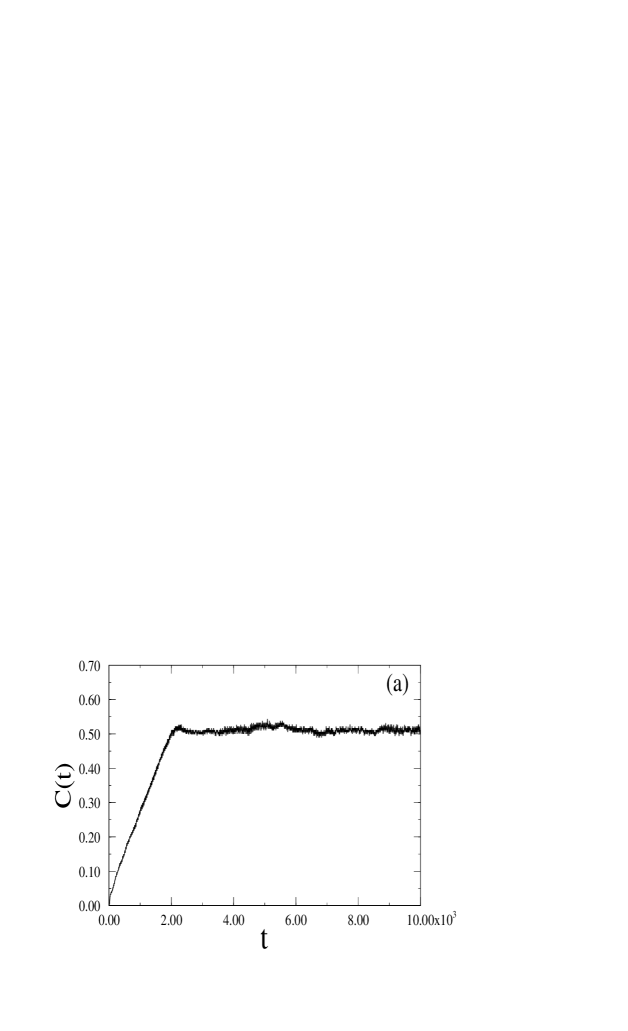
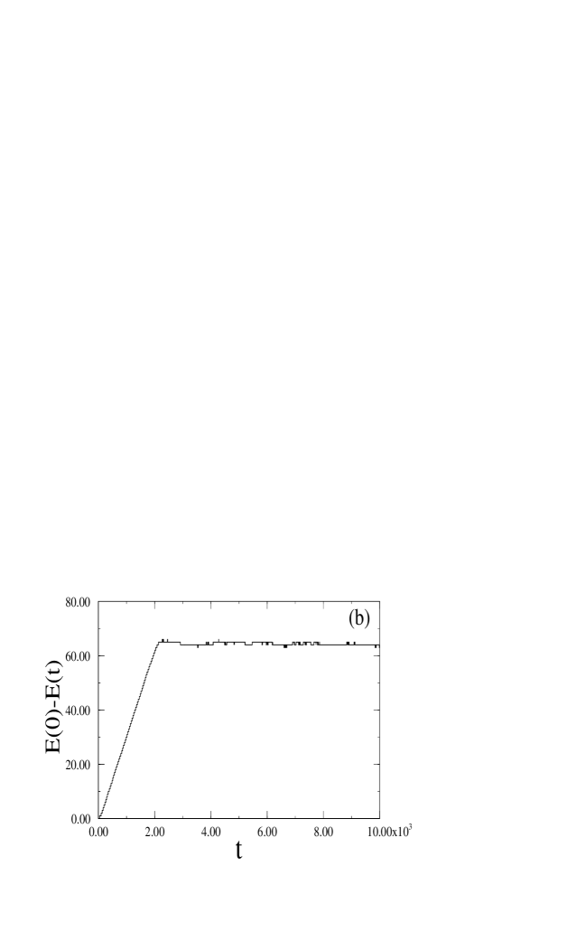
Figure 3: (a) The density contrast C(t) versus time step t. (b) Kinetic energy loss $E(0)-E(t)$ versus time step t. Here E(0) is the kinetic energy at t=0. The kinetic energy of a moving particle is chosen as energy unit.

where K is the number of bins we divided the pipe into and $\bar{n}$ is the average number of particles in a bin. The periodic boundary condition ensures $n_{K+1}=n_{1}$. In figure 3 (a) we plot the density contrast $C(t)$ versus time step $t$. This curve was obtained by averaging over 64 simulations for systems with length $L=256$, width $W=11$. It is clear that the density contrast increases from zero before it saturates at a fixed value, indicating that the density waves are being formed spontaneously from the uniform initial configurations. In figure 3 (b) the relexation of the kinetic energy $E(t)$ of the system is plotted. We take the kinetic energy of one particle to be unity. Since the particles have a kinetic energy of either one (for moving particles) or zero (for rest particles) in our LGA model, the loss of kinetic energy due to dissipation is equal to the increase in the number of rest particles. We see from figure 3 (b) that the system loses its kinetic energy in the early stage and then reaches a steady state where the kinetic energy loss due to dissipation is compensated by the work of gravity (i.e. the potential energy loss).

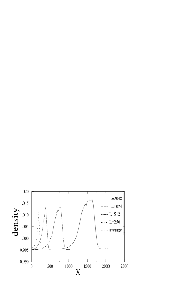
Figure 4: Density as a function of position X along the pipe. The average has been made in the perpendicular direction. The model parameters are $\rho=1.0$, $p=0.1$, $g=0.5$, $b=0.5$. The width is fixed for various pipe lengths, $W=11$.

From figure 2 we know that there is a strongest density wave which is quite different from the rest. To obtain the shape of this density wave, we did many simulations and averaged. For each system size, we run $64$ simulations. For each simulation run, we recorded the density field at each time step in the steady state to keep $2048$ density fields. The density fields are then shifted vertically so that they overlap each other maximally. Since the density wave travels along the pipe, this shifted distance should be equal to the time interval of the two density fields multipied by the average velocity in that time interval. We use this shift distance to determine the velocity of the density wave in the next subsection. Here the maximal overlap rule is applied hierarchically to obtain a clearer shape of the density wave. $64$ simulation runs are then averaged to give the final density profiles which are presented in figure 4. We notice that the density wave has a non–symmetric shape and its wave front is sharper than the backside of the wave. The width of the wave also has a scaling relation with the system length (almost linear) and the amplitude of the wave only increases a little bit as the system length increases. A similar density profile was produced in Ref. [27] with a lattice Boltzmann model.

C. Density Wave Velocity

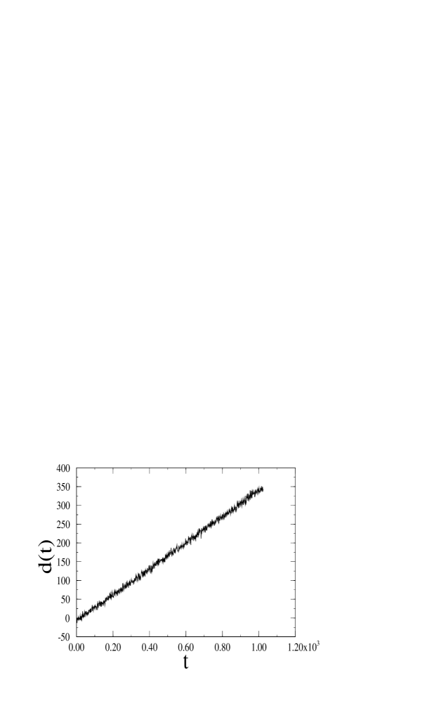
Figure 5: Real–space determination of the velocity of density wave. The horizontal axis is the time interval while the vertical axis is the displacement of the wave obtained by maximal overlap. The velocity is the slope of the line which is $0.36\pm 0.05$ for a system with $L=512$, $W=11$, $\rho=1.0$, $p=0.1$, $g=0.5$, $b=0.5$.

As mentioned above, the velocity of the density wave can be measured by the distance shifted along the pipe to make maximal overlap. If one divides the shifted distance by the time interval, one will obtain the average velocity in this time interval. However, we can not be $a\hskip 3.0ptpriori$ sure that the velocity is constant all the time steps. So, alternatively we first chose a reference scheme and then distance and time are measured from this reference scheme. The velocity was measured by plotting the shifted distance versus the shifted time. In figure 5 such a distance–versus–time plot is shown. This plot is obtained by averaging 64 simulation runs each consisting of 2048 density fields. The linearity of this curve indicates that the density wave propagate along the pipe with a constant velocity. The velocity is the slope of the line. This is a real–space determination of the velocity. In the next subsection we will give another method of measuring the velocity which is a by–product of the Fourier transformation. In the following we determine all the velocities by this Fourier transformation method and we have checked that the results given by the two methods coincide.

D. $1/f$ noise in the density fluctuation

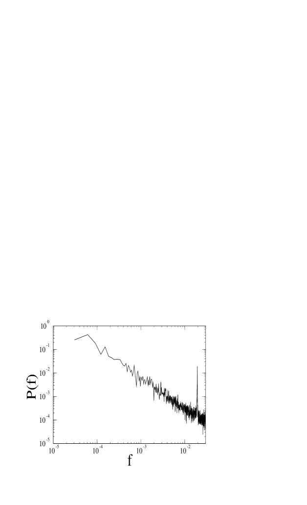
Figure 6: Power spectrum $P(f)$ of the time series of the density fluctuation inside a region in a pipe of length L=220 and width W=11. The model parameters are $p=0.8$, $b=0.5$, $g=0.5$, $\rho=1.0$. The time series of the density fluctuation were recorded every 10 time steps and the time period correponding to a frequency $f$ is $10/f$.

To characterize the density fluctuations in a certain region with time, we calculate their power spectra. We recorded the number of particles in a bin. The LGA is performed for very long time steps so that we obtain good statistics to analyse each power spectrum. We first substract the mean value from the data, otherwise there would be a huge peak at $f=0$ in the power spectra. We calculated the spectra using a standard FFT routine. The power is essentially the square of the amplitude of the Fourier Transformation of a time series. But to get better statistics, average process has been used. We broke the time series into $S$ segments of $M$ points each. On each segment an FFT was performed using a Parzen window [28] and the powers of the resulting spectra were averaged. We used $S=4$ and $M=16384$ for most of the results. One representative power spectrum is shown in figure 6 for systems with $g=0.5,b=0.5,\rho=1.0$ and $p=0.8$. In this figure we observe a sharp peak. This peak is due to the contribution of the strongest density wave observed in figure 2. The frequency of this peak corresponds to a wave velocity of $Lf/T_{0}$ where $L$ is the pipe length and $T_{0}$ is the time interval of recording (we recorded the data every $T_{0}=10$ time steps). The velocity measured in this way coincides with the direct measurement in real space (see above subsection). Apart from this peak one sees that there is a background having a power law behaviour where the spectrum falls off as $1/f^{\alpha}$. The exponent $\alpha$ is found to be around 1.33 for the parameters used in figure 6. The power–law decay in the power spectra was also observed in experiments [12, 11, 16]. In the following subsections we will show how the exponent and the velocity depend on the parameters $(p,\rho,g$, and $b)$.

E. White Noise

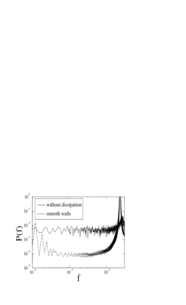
Figure 7: Power spectra $P(f)$ of the time series of the density fluctuation inside a region in a pipe of length L=220 and width W=11. Either without dissipation or with smooth walls, white noise is observed. The model parameters for the system without dissipation are $p=0$, $b=0.5$, $g=0.5$, $\rho=1.0$ while $p=0.5$, $b=0$, $g=0.5$, $\rho=1.0$ for the system with smooth walls.

As we reported in [24], both dissipation and the roughness of walls are the neccessary conditions for the presence of travelling density waves. To see whether the $1/f$ noise is associated to the density waves, we also performed the power spectra for systems without dissipation ($p=0$) and sytems without roughness on the walls ($b=0$). These results are shown in figure 7 where we see white noise. The large peak in the spectrum for system without roughness on the walls is due to the fact that particles are perfectly reflected on the walls, generating a wave–like motion of density along the pipe (the velocity of this peak is exactly $1/2$ which is a geometric effect of the lattice used). White noise is also experimentally observed when the walls are smooth [16]. Together with our earlier results [24], figure 7 shows that the $1/f^{\alpha}$ noise is associated with the density waves.

F. Dependence on Dissipation

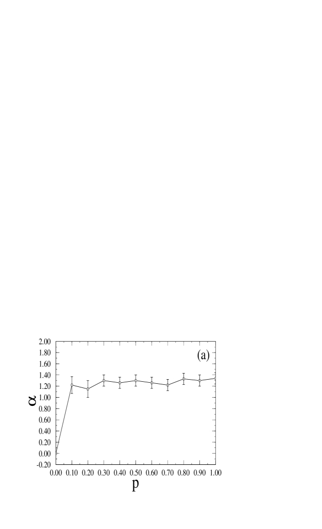
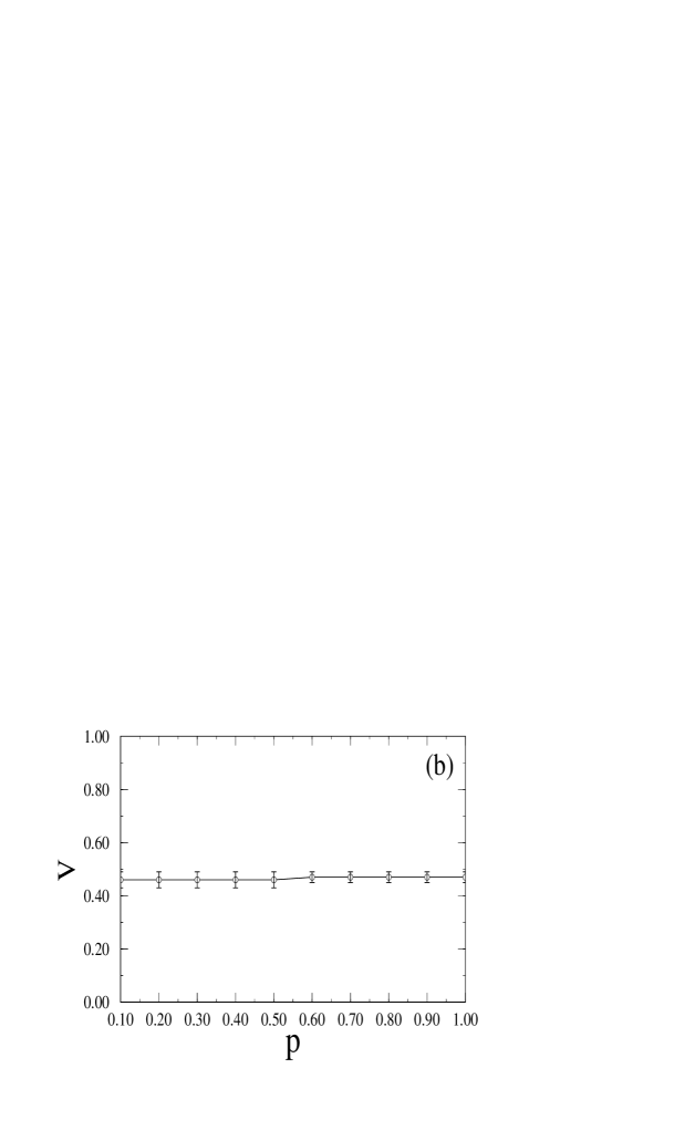
Figure 8: Dependence on the dissipation parameter $p$. The model parameters kept fixed are $b=0.5$, $g=0.5$ and $\rho=1.0$. (a) The power–law decay exponent $\alpha$ of the power spectra. (b) The velocity of the density wave.

From above we know that for systems without dissipation the power spectra are just white noise, i.e, $\alpha=0$. How does the exponent $\alpha$ change with the dissiption parameter $p$ of our model? In figure 8 (a) we show the dependence of $\alpha$ on $p$. Each exponent in this figure was extracted from the average power spectra of 32 simulation runs, thus ensuring acceptable error bars. The other parameters which are kept fixed are respectively: $\rho=1.0$, $b=0.5$, $g=0.5$. From figure 8 we see that the exponent of the power–law decay in the spectra has approximately a constant value provided that there is dissipation in the granular system. Without dissipation, $\alpha$ would be zero. The exponent jumps to a constant value when $p$ changes from zero to a non-zero value. From this point of view, this figure reinforces the idea that the mere existence of dissipation can give rise to a significant change in the physics of the system even if the degree of dissipation is minute [26, 24]. In Ref. [24] we provided another explaination to this idea, i.e., the density waves disappear when the system has no dissipation.

Figure 8 (b) shows that the velocity of the density wave does not change with dissipation within the error bars. The parameters used for the model and the averaging are the same as for figure 8 (a).

Using a Kolmogorov–Obukhov approach revised for space–intermittent systems, Bershadskii [29] proposed that the exponent which we found to be around $1.33$ for our model [24] might be an universal value of $4/3$ for scalar fluctuations convected by stochastic velocity fields in dissipative systems. Our numerical results for the present LGA model show that the exponent does not change with $p$, $b$ and $g$ (see the following subsections), but the average density $\rho$ does affect the exponent and this will be discussed in the next subsection.

G. Dependence on Average Density

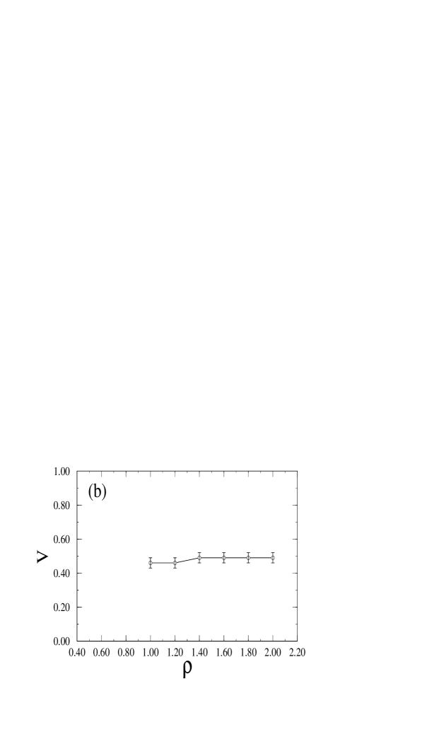
Figure 9: Dependence on the average density $\rho$. The model parameters kept fixed are $p=0.5$, $b=0.5$ and $g=0.5$. (a) The power–law decay exponent $\alpha$ of the power spectra. (b) The velocity of the density wave.

In figure 9 (a) we show how the exponent depends on the average density $\rho$. For very low density ($\rho\leq 0.8$) the exponent is zero, thus the density fluctuation in the pipe is just white noise. Since in this density region the interaction among the particles is so weak that no collective motion can be formed, the exponent can be easily understood. For average densities above $1.0$, the exponent increases with $\rho$. We found $\alpha\approx 1.86$ when $\rho=2.0$. We did not go beyond $\rho=2.0$ since our LGA model becomes less valid as the average density becomes higher. In the present model we introduced a rest state which can be occupied only by one particle. Therefore, the model is not valid when the number of rest particles exceedes the total number of sites. When the average density increases high enough, the number of rest particles due to the fixed dissipation rate $p$ might be too large so that the model becomes less valid for granular flow.

The velocity of the density wave is constant when the average density changes. This is shown in figure 9 (b).

H. Dependence on Boundary Roughness and Gravity

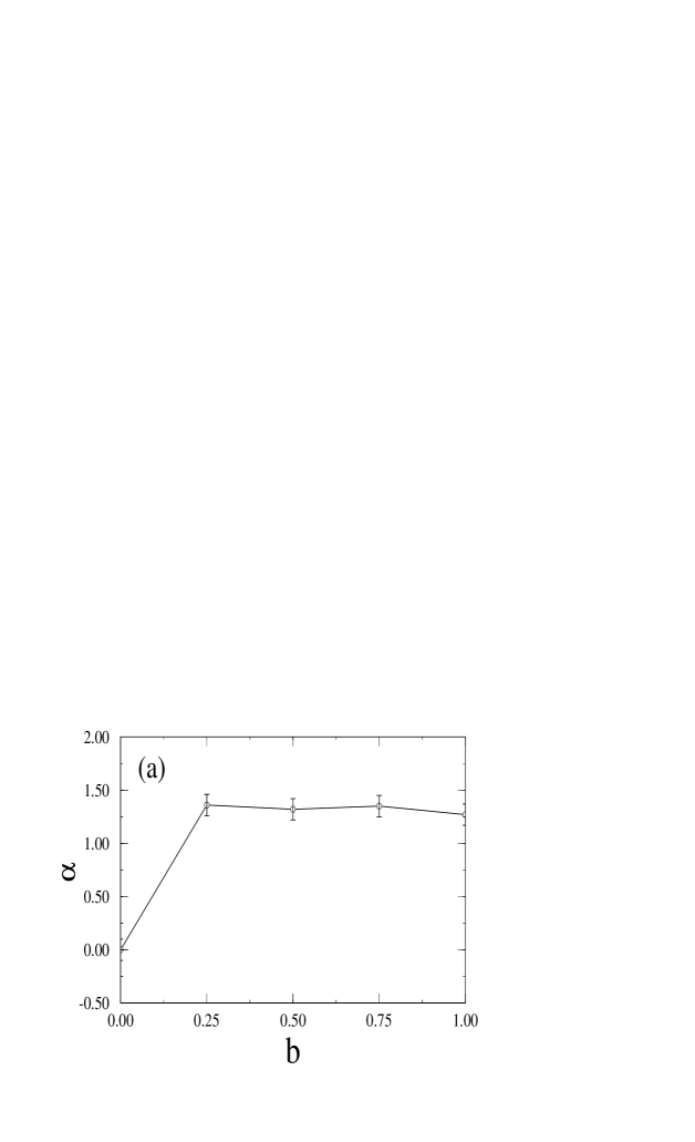
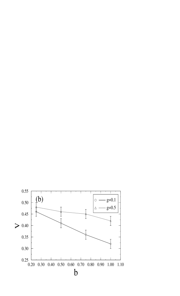
Figure 10: Dependence on the roughness $b$ of the walls. (a) Power–law decay exponent $\alpha$ in the power spectra. The model parameters kept fixed are $p=0.5$, $g=0.5$ and $\rho=1.0$. (b) Velocity of the density wave for two different magnitudes of gravity. Here $p=0.5$ and $\rho=1.0$.

As we noted in Ref. [24] and discussed in subsection E, the roughness of the walls is essential to the formation of density waves. Without roughness, no density waves propagates in the system. We calculated the power spectra for such cases and found that the density fluctuation is white noise and the exponent $\alpha=0$. When the roughness parameter $b$ is turned on even if b is very small, the power spectrum changes. The exponents $\alpha$ are constant for any non–zero value of $b$. This phenomenon is illustrated in figure 10 (a). Changing gravity magnitude we found no change in the exponent.

In figure 10 (b) we present two curves to show how the velocity of the density wave varies with the roughness of the walls and the magnitude of gravity. The upper curve shows that the velocity decreases a little bit as $b$ increases from $0.25$ to $1.0$. This small difference is due to the fact that the applied gravity is large enough to dominate the velocity. As the magnitude of gravity becomes smaller the velocity is more sensitive to the roughness of walls as shown in the lower curve of figure 10 (b). These two curves also show that the velocity changes with gravity. All these results are reasonable to our daily experienece. For experimentist, to change the magnitude of gravity can be performed by putting the system on an oblique desk instead of letting the pipe vertical.

I. Open Systems

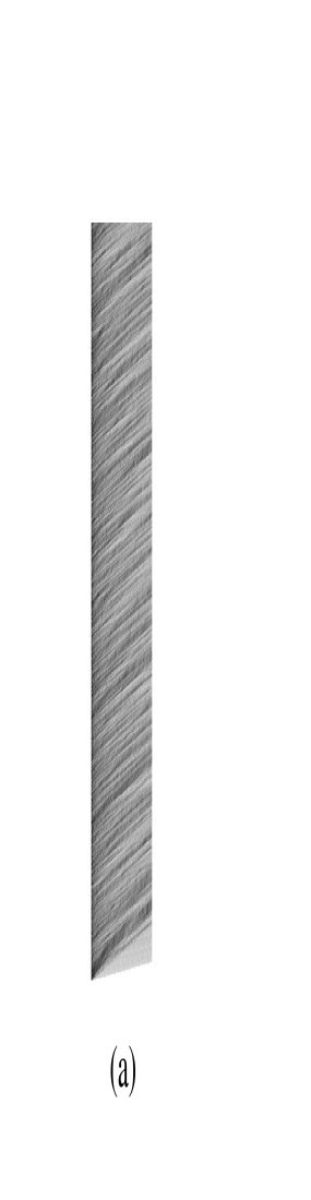
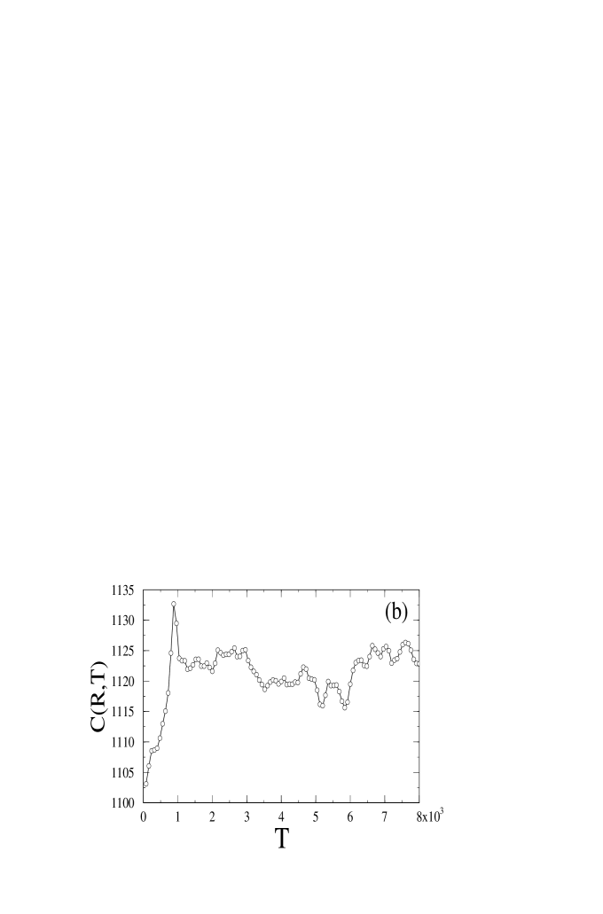
Figure 11: (a) Time evolution of the density $n_{i}\{i=1,2,\cdots 220\}$ in the $100$ bins in the pipe of $L=1000$, $W=5$ and $I=0.5$. Other model parameters are $p=0.5$, $b=0.5$, $g=0.2$. Densities at a given time are plotted from left to right (direction of gravity) while densities at different time steps are plotted from bottom to top (direction of time increase). Time goes from $0$ to $40,000$ time steps. The grayscale of each bin is a linear function of $n_{i}$. Darker regions correspond to higher densities. (b) Two–point density–density correlation function $C(R,T)$ versus time difference $T$ at a fixed spatial separation $R=30$ for the evolution shown in (a).

From the experimental point of view, open boundary condition is more realistic than the periodic boundary condition. Here we consider open systems. The LGA for open systems is defined in analogy with the model described in section II, with the exception that the periodic boundary condition in the vertical direction is replaced by an open boundary condition. Initially the pipe is empty. Particles are then injected from the upper boundary by a constant rate $I$ and leave the system at the lower boundary without coming back. The injection rate is defined as follows. On each site of the upper boundary we consider the states whose corresponding velocities point into the system. If such a state is not occupied, it can be filled with probability of $I$. A time–evolution of the density in the pipe is shown in figure 11 (a). Densities at a given time are plotted from left to right while densities at different time are plotted from bottom to top as time increases. Gravity acts from left to right. From this plot we observe that high density regions can also be formed in open systems. These high density regions may travel along the pipe until they leave the system from the lower border or they may die out during their propagation. There are also more than one high density regions at one time, in contrast to what we observed in figure 2 in periodic systems. It seems to us that all the density waves travel with a constant velocity in figure 11 (a). So we measure this velocity using density–density correlation function which is defined as:

$$C(R,T)=\sum_{i,t}{n_{i}(t)n_{i+R}(t+T)}$$ (2)

where $n_{i}(t)$ is the number of particles in the i’th bin at time step $t$. In figure 11 (b) we plot the correlation function against the time difference $T$ for a fixed spatial separation $R=30$. An observable peak exists at $T_{c}=880$ in the correlation function which gives the velocity of the density waves $v=R\delta/T_{c}=0.34$ where $\delta=10$ is the length of a bin.

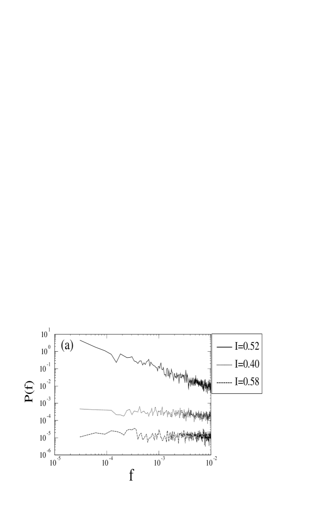
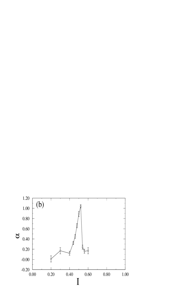
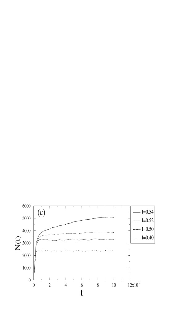
Figure 12: (a) Three typical power spectra for different injection rates $I$, $I=I_{c}=0.52,I<I_{c},I>I_{c}$. The model parameters kept fixed are $p=0.5$, $b=0.5$, $g=0.5$. The two lower curves have been shifted vertically for clarity. (b) The exponent $\alpha$ in the power spectra $1/f^{\alpha}$ for different injection rates. (c) Total number of particles in the system $N(t)$ versus time step $t$ for different injection rates. Each curve is an average over $32$ simulations.

We have measured the density fluctuation in a bin very close to the bottom of the pipe. Its power spectrum is found to follow $1/f$ noise only around a critical injection rate $I_{c}=0.52$ and white noise otherwise. Figure 12 (a) shows three power spectra for different injection rates, $I=I_{c}$, $I<I_{c}$ and $I>I_{c}$. The power spectrum for $I=I_{c}$ falls off with a slope close to -1 in the log–log plot. The exponent $\alpha$ for the power spectra $1/f^{\alpha}$ is shown in figure 12 (b) for different injection rates $I$. It seems that the power spectrum is $1/f$ noise only at the critical point. The critical injection rate is found to be independent of the model parameters and the system sizes. We guess it might be dependent on the lattice (here trianglar lattice is used).

To identify what the critical injection rate means, we investigate the nature of the two phases seperated by the critical injection rate. We find that in the phase for $I>I_{c}$ the system is clogging while for $I<I_{c}$ particles pass the system freely without clogging. Figure 12 (c) shows the total number of particles in the system for different injection rates. It is clear that the total number of particles increases with time in the very early stage for every injection rate. This is due to the fact that we simulate the process starting from an empty pipe. After this relaxation time, the system reaches a steady state for $I<I_{c}$ where the number of incoming particles is on average equal to that of outgoing particles, thus keeping the total number of particles in the system constant. However, for $I=0.54$ which is slightly larger than $I_{c}=0.52$, the total number of particles increases all the time, meaning that some particles accumulate in the system. Thus, the phase for $I>I_{c}$ can be identified as a clogging phase. It is therefore seems that $I_{c}$ is the maximal injection rate that the system can sustain without clogging. In Ref. [30] Vermöhlen $et\hskip 2.0ptal$ also found a critical inflow rate into a hopper with the time–to–clog diverging at the critical point.

IV. Disscussion

Using a simple lattice–gas automaton model we have shown that density waves can be formed either from uniform initial conditions in the periodic case or by injecting particles into an open system. Energy dissipation is an important factor for this kind of instability. Goldhirsch and Zanetti [26] have shown that a gas composed of dissipative particles is unstable to the formation of high density clusters. They have observed clusters of high density in a system without an external field (like gravity). Here we observe high density regions travelling in the system under the action of gravity. Density waves were also observed in traffic jam models [31] which might bear some relevance to granular systems.

The density fluctuations in our systems are found to follow $1/f^{\alpha}$ noise with $0\leq\alpha\leq 2$. Power–law spectra have also been observed in experiments [11, 12, 16] and MD simulations [14]. It is clear from our numerical results that $1/f^{\alpha}$ spectra with $\alpha\neq 0$ are associated with the propagation of density waves. In the simulation of open systems, we find a critical injection rate. At the critical point the system has its maximal throughput without clogging. In experiments one usually has a hopper above the pipe to ensure constant refilling. Particles flow into the pipe by the action of gravity and in fact particles flow down at the maximum rate. That is to say, the system has its maximal outflow, which means the system self–organizes into the critical state at $I_{c}$. At the critical state the density fluctuation follows a $1/f$ noise. The explanation of the ubiquitous $1/f$ noise in granular flow is open. In the traffic jam model, Nagel [32] also found the state of maximal throughput to be critical.

We note here that the construction of the LGA model is not unique. Károlyi and Kertész [33] have independently designed an LGA model where the rest particles are located in the bonds in addition to the rest particles on the sites. The use of LGA models to study other phenomena in granular materials (e.g., the pile of sand or convection under vibration) is in progress [34].

We thank Stephan Melin, Cristian Moukarzel, Thorsten Pöschel, Stefan Schwarzer, Hans-Jürgen Tillemans and Wolfgang Vermöhlen for useful discussions.

Figure Captions

Figure 1: (a) Probabilistic collision rules for two– and three–body collisions. Thin arrows represent particles and small circles stand for rest particles. The number next to a configuration is the probability that the configuration takes place; (b) Collision rules for moving particles with a rest particle. Immediately after the collision, more than one rest particle on a site will hop to the nearest neighbouring sites randomly until they find a suitable site with no rest particle already there. (c) Gravity may change the momentum of the particle by a unit vector in the direction of gravity. (d) Collision rule for a moving particle colliding with the wall.

Figure 2: Time evolution of the density $n_{i}\{i=1,2,\cdots 220\}$ divide in $220$ bins along the pipe of $L=2200$, $W=11$ and $\rho=1.0$. Densities at a given time are plotted from left to right (direction of gravity) while densities at different time steps are plotted from bottom to top (direction of time increase). (a) 9 successive snapshots every 2,000 time steps from $t=0$; (b) Time–evolution every 80 time steps during $40,000$ time steps. The grayscale of each bin is a linear function of $n_{i}$. Darker regions correspond to higher densities.

(a)

(b)

(c)

(d)

Figure 1: (a) Probabilistic collision rules for two– and three–body collisions. Thin arrows represent particles and small circles stand for rest particles. The number next to a configuration is the probability that the configuration takes place; (b) Collision rules for moving particles with a rest particle. Immediately after the collision, more than one rest particle on a site will hop to the nearest neighbouring sites randomly until they find a suitable site with no rest particle already there. (c) Gravity may change the momentum of the particle by a unit vector in the direction of gravity. (d) Collision rule for a moving particle colliding with the wall.

Figure 2: Time evolution of the density $n_{i}\{i=1,2,\cdots 220\}$ divide in $220$ bins along the pipe of $L=2200$, $W=11$ and $\rho=1.0$. Densities at a given time are plotted from left to right (direction of gravity) while densities at different time steps are plotted from bottom to top (direction of time increase). (a) 9 successive snapshots every 2,000 time steps from $t=0$; (b) Time–evolution every 80 time steps during $40,000$ time steps. The grayscale of each bin is a linear function of $n_{i}$. Darker regions correspond to higher densities.

Figure 3: (a) The density contrast C(t) versus time step t. (b) Kinetic energy loss $E(0)-E(t)$ versus time step t. Here E(0) is the kinetic energy at t=0. The kinetic energy of a moving particle is chosen as energy unit.

Figure 4: Density as a function of position X along the pipe. The average has been made in the perpendicular direction. The model parameters are $\rho=1.0$, $p=0.1$, $g=0.5$, $b=0.5$. The width is fixed for various pipe lengths, $W=11$.

Figure 5: Real–space determination of the velocity of density wave. The horizontal axis is the time interval while the vertical axis is the displacement of the wave obtained by maximal overlap. The velocity is the slope of the line which is $0.36\pm 0.05$ for a system with $L=512$, $W=11$, $\rho=1.0$, $p=0.1$, $g=0.5$, $b=0.5$.

Figure 6: Power spectrum $P(f)$ of the time series of the density fluctuation inside a region in a pipe of length L=220 and width W=11. The model parameters are $p=0.8$, $b=0.5$, $g=0.5$, $\rho=1.0$. The time series of the density fluctuation were recorded every 10 time steps and the time period correponding to a frequency $f$ is $10/f$.

Figure 7: Power spectra $P(f)$ of the time series of the density fluctuation inside a region in a pipe of length L=220 and width W=11. Either without dissipation or with smooth walls, white noise is observed. The model parameters for the system without dissipation are $p=0$, $b=0.5$, $g=0.5$, $\rho=1.0$ while $p=0.5$, $b=0$, $g=0.5$, $\rho=1.0$ for the system with smooth walls.

Figure 8: Dependence on the dissipation parameter $p$. The model parameters kept fixed are $b=0.5$, $g=0.5$ and $\rho=1.0$. (a) The power–law decay exponent $\alpha$ of the power spectra. (b) The velocity of the density wave.

Figure 9: Dependence on the average density $\rho$. The model parameters kept fixed are $p=0.5$, $b=0.5$ and $g=0.5$. (a) The power–law decay exponent $\alpha$ of the power spectra. (b) The velocity of the density wave.

Figure 10: Dependence on the roughness $b$ of the walls. (a) Power–law decay exponent $\alpha$ in the power spectra. The model parameters kept fixed are $p=0.5$, $g=0.5$ and $\rho=1.0$. (b) Velocity of the density wave for two different magnitudes of gravity. Here $p=0.5$ and $\rho=1.0$.

Figure 11: (a) Time evolution of the density $n_{i}\{i=1,2,\cdots 220\}$ in the $100$ bins in the pipe of $L=1000$, $W=5$ and $I=0.5$. Other model parameters are $p=0.5$, $b=0.5$, $g=0.2$. Densities at a given time are plotted from left to right (direction of gravity) while densities at different time steps are plotted from bottom to top (direction of time increase). Time goes from $0$ to $40,000$ time steps. The grayscale of each bin is a linear function of $n_{i}$. Darker regions correspond to higher densities. (b) Two–point density–density correlation function $C(R,T)$ versus time difference $T$ at a fixed spatial separation $R=30$ for the evolution shown in (a).

Figure 12: (a) Three typical power spectra for different injection rates $I$, $I=I_{c}=0.52,I<I_{c},I>I_{c}$. The model parameters kept fixed are $p=0.5$, $b=0.5$, $g=0.5$. The two lower curves have been shifted vertically for clarity. (b) The exponent $\alpha$ in the power spectra $1/f^{\alpha}$ for different injection rates. (c) Total number of particles in the system $N(t)$ versus time step $t$ for different injection rates. Each curve is an average over $32$ simulations.

References

- [1] J. C. Williams, Powder Technol.15, 245 (1976).
- [2] P. K. Haff and B. T. Werner, Powder Technol.48, 239 (1986).
- [3] A. Rosato, K. J. Strandburg, F. Prinz, and R. H. Swendsen, Phys. Rev. Lett. 49, 59 (1987).
- [4] P. Devillard, J. Phys. France 51, 369 (1990).
- [5] M. Faraday, Philos. Trans. R. Soc. London 52, 299 (1831).
- [6] P. Evesque and J. Rajchenbach, Phys. Rev. Lett. 62, 44(1989).
- [7] Y. H. Taguchi, Phys. Rev. Lett. 69, 1367(1992).
- [8] J. A. C. Gallas, H. J. Herrmann, and S. Sokolowski, Phys. Rev. Lett. 69, 1371(1992).
- [9] C–h. Liu and S. R. Nagel, Phys. Rev. Lett. 68, 2301(1992).
- [10] H. M. Jaeger and S. R. Nagel, Science 255, 1523(1992).
- [11] K. L. Schick and A. A. Verveen, Nature 251, 599(1974).
- [12] G. W. Baxter, R. P. Behringer, T. Fagert, and G. A. Johnson, Phys. Rev. Lett. 62, 2825(1989).
- [13] T. Pöschel, J. Phys. I France, 4, 499(1992).
- [14] G. Ristow and H. J. Herrmann, Phys. Rev. E 50, R5(1994).
- [15] J. Lee, Phys. Rev. E 49, 281(1994).
- [16] P. Dimon, Private Communication.
- [17] C. S. Campbell and C. E. Brennen, J. Fluid Mech. 151, 167(1985); P. A. Thompson and G. S. Grest, Phys. Rev. Lett. 67, 1751(1991); D. M. Hanes and D. L. Inman, J. Fluid Mech. 150, 357(1985); O. R. Walton and R. L. Braun, J. Rheol. 30, 949(1986).
- [18] J. Lee and H. J. Herrmann, J. Phys. A 26, 373(1993).
- [19] A. Rosato, K. J. Strandburg, F. Prinz and R. H. Swendsen, Phys. Rev. Lett. 58, 1038(1987); A. D. Rosato, Y. Lan and D. T. Wang, Powder Technol. 66, 149(1991).
- [20] S. Luding, E. Clément, A. Blumen, J. Rajchenbach and J. Duran, Phys. Rev. E 49, 1634(1994).
- [21] G. W. Baxter and R. P. Behringer, Phys. Rev. A 42, 1017(1990); Physica D 51, 465(1991).
- [22] M. P. Allen and D. J. Tildesley, Computer Simulations of Liquids, Clarendon Press, Oxford (1987).
- [23] U. Frisch, B. Hasslacher, and Y. Pomeau, Phys. Rev. Lett. 56, 1505(1986).
- [24] G. Peng and H. J. Herrmann, Phys. Rev. E 48, R1796(1994).
- [25] S. Savage, J. Fluid Mech. 241, 109(1992).
- [26] I. Goldhirsch and G. Zanetti, Phys. Rev. Lett. 70, 1619(1993).
- [27] E. Flekkøy and H. J. Herrmann, Physica A 199, 1(1993).
- [28] W. H. Press, B. P. Flannery, S. A. Teukolsky, and W. T. Vetterling, Numerical Recipes in C, Cambridge University Press, Cambridge (1988).
- [29] A. Bershadskii, preprint (1994).
- [30] W. Vermöhlen, G. A. Kohring, S. Melin, H. Puhl and H. J. Tillemans, HLRZ preprint, 75/93, (1993)
- [31] K. Nagel and M. Schreckenberg, J. Physique I 2, 2221(1992).
- [32] K. Nagel, Int. J. Mod. Phys. C 5, 567(1994).
- [33] A. Károlyi and K. Kertész, preprint, (1994).
- [34] H. J. Herrmann, in preparation.