Neutron scattering in a d_x^2-y^2–wave superconductor with strong impurity scattering and Coulomb correlations

Abstract

We calculate the spin susceptibility at and below $T_{c}$ for a $d_{x^{2}-y^{2}}$–wave superconductor with resonant impurity scattering and Coulomb correlations. Both the impurity scattering and the Coulomb correlations act to maintain peaks in the spin susceptibility, as a function of momentum, at the Brillouin zone edge. These peaks would otherwise be suppressed by the superconducting gap. The predicted amount of suppression of the spin susceptibility in the superconducting state compared to the normal state is in qualitative agreement with results from recent magnetic neutron scattering experiments on La_1.86Sr_0.14CuO₄ for momentum values at the zone edge and along the zone diagonal. The predicted peak widths in the superconducting state, however, are narrower than those in the normal state, a narrowing which has not been observed experimentally.

I Introduction

Recent magnetic neutron scattering experiments on La_1.86Sr_0.14CuO₄ by Mason and co-workers[1] show an isotropic but incomplete suppression of the scattering intensity below $T_{c}$ for small energy transfers and momentum transfers near the $(\pi,\pi)$ point of the Brillouin zone. In the normal state, the magnetic neutron scattering intensity, as a function of momentum, exhibits four peaks displaced slightly along the edges of the Brillouin zone away from the $(\pi,\pi)$ point at the corner of the zone, as shown in Fig. 1.

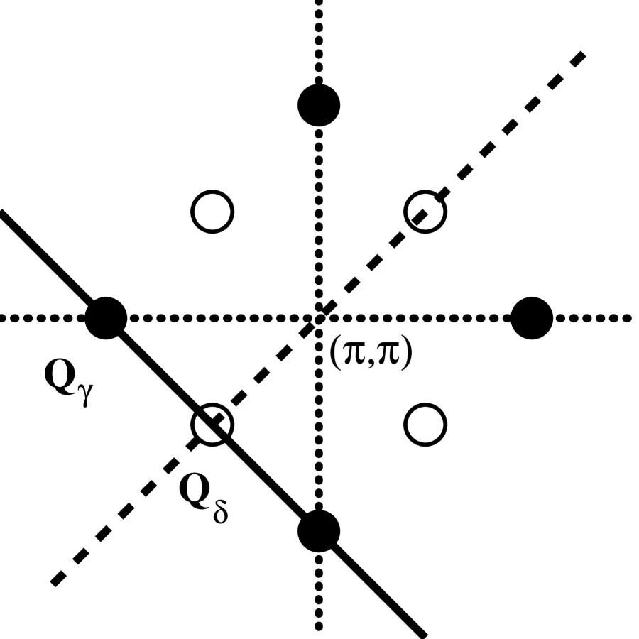
FIG. 1.: Map of reciprocal space probed by the neutron scattering experiments. Dotted lines represent the Brillouin zone edges near the $(\pi,\pi)$ point. The dashed line indicates the zone diagonal. Filled circles show the locations of neutron scattering intensity peaks in the normal state. Open circles represent the expected positions for scattering intensity peaks for a clean $d$–wave superconductor well below $T_{c}$. The solid line shows the direction of the momentum scans shown in Fig. 5 and Figs. 10-12.

The experimental results show a suppression of these peaks, compared to their magnitude at $T_{c}$, of about 60% at a temperature of $0.13T_{c}$.

For an isotropic $s$–wave superconductor we would expect an isotropic suppression of this scattering intensity as the temperature drops below $T_{c}$. But for a clean $s$–wave state at low temperatures the intensity should die away exponentially with temperature. The moderate suppression shown by experiment suggests that if $s$–wave superconductivity is present, it is gapless and isotropic.

Alternatively, a superconductor with $d_{x^{2}-y^{2}}$ symmetry is always gapless, so an incomplete suppression of the scattering intensity is to be expected. However, for a clean $d$–wave superconductor it is expected that this suppression will not be isotropic. Lu[2] and Zha and co-workers[3] have pointed out that in the superconducting state the four normal state peaks should be suppressed, leaving only the response due to particle-hole excitations associated with the nodes. This response is displaced slightly away from $(\pi,\pi)$ along the zone diagonals, giving a low temperature structure which appears to have undergone a 45 degree rotation about $(\pi,\pi)$. The failure to observe this rotation has raised questions regarding whether a $d_{x^{2}-y^{2}}$ description of the superconducting state of La_2-xSr_xCuO₄ is viable.

Now, for $d_{x^{2}-y^{2}}$ pairing it is known that resonant impurity scattering leads to important effects for both the penetration depth[4] and the NMR response.[5] In addition, the effects of the Coulomb enhanced spin fluctuations are believed to play an essential role in the cuprates. As previously discussed,[6, 7] when the effects of Coulomb correlations on the magnetic neutron scattering are included within the RPA approximation, the $d_{x^{2}-y^{2}}$ results can be brought into closer agreement with the experimental observations.

Here we investigate both of these effects by calculating the neutron scattering for a model of a dirty $d_{x^{2}-y^{2}}$–wave superconductor with strong Coulomb correlations. Specifically, we consider a Hubbard model on a two-dimensional square lattice with a near-neighbor hopping $t$ and an on-site Coulomb interaction $U$. To this we add impurity scattering in the form of a dilute random array of zero-range scattering potentials $V$.

The magnetic neutron scattering intensity is given by a structure factor $S({\bf q},\omega)=[n(\omega)+1]\chi^{\prime\prime}({\bf q},\omega)$, which is proportional to the imaginary part of the spin susceptibility $\chi({\bf q},\omega)$. We calculate $\chi({\bf q},\omega)$ in two stages. First, in Sec. II, we examine the effects of the impurities on $\chi({\bf q},\omega)$, including self-energy as well as vertex corrections. Then, in Sec. III, the strong spin susceptibility enhancement effects of the Coulomb interaction are included within an RPA-type approximation. Section IV contains our conclusions.

Before beginning, it is useful to review the behavior expected for a system described by a two-dimensional tight-binding band which undergoes a transition from a normal state to a $d_{x^{2}-y^{2}}$ BCS superconducting state in the absence of impurity scattering and strong Coulomb correlations. As discussed in Littlewood et al.,[8] the four normal state peaks shown in Fig. 1 arise due to a combination of the weak requirements for favorable nesting in two dimensions combined with umklapp scattering processes. As a $d$–wave gaps opens up below $T_{c}$ the thermally available scattering states are restricted to those near the nodes of the $d$–wave gap function and these peaks are suppressed. The favorable low-energy momentum transfers are then restricted to those which represent node-to-node scattering, and the corresponding wavevectors lie along the zone diagonal directions. Thus at low temperatures and energies well below $2\Delta(0)$, peaks in the neutron scattering should be observed to lie along the zone diagonals.[2, 3]

Here we find that impurity scattering and Coulomb correlations both act to keep the scattering intensity peaks at their normal state positions along the Brillouin zone edge. For reasonable parameters, the amount of suppression of the scattering intensity in the dirty–$d_{x^{2}-y^{2}}$ superconducting state compared to the normal state is consistent with the experimental observations both at the zone edge and along the diagonal. However, the predicted peak widths in the superconducting state are narrower than those in the normal state, a narrowing which has not been observed experimentally.

II Impurity scattering effects

In this section we examine the effect of impurities on the spin susceptibility of a BCS $d_{x^{2}-y^{2}}$ state. We begin by including the self-energy effects and then consider the impurity vertex corrections.

A Self-energy corrections

Neglecting the vertex corrections, the spin susceptibility in the superconducting state is given by the particle-hole bubble diagrams shown in Fig. 2.

FIG. 2.: Lowest order bubble diagram representing the spin susceptibility probed in magnetic neutron scattering experiments.

The bare vertex representing magnetic neutron scattering is understood to connect only electrons of opposite spin. Evaluating this diagram, continuing to real frequencies, and taking the imaginary part, we obtain the following formula for $\chi^{\prime\prime}({\bf q},\omega)$:

$$\chi^{\prime\prime}({\bf q},\omega)=-\pi\int{d^{2}p\over(2\pi)^{2}}~{}d\omega^{\prime}~{}[f(\omega+\omega^{\prime})-f(\omega^{\prime})]~{}[ A_{N}({\bf p}+{\bf q},\omega+\omega^{\prime})A_{N}({\bf p},\omega^{\prime})$$ (2)

$$+A_{A}({\bf p}+{\bf q},\omega+\omega^{\prime})A_{A}({\bf p},\omega^{\prime})].$$

$A_{N}({\bf p},\omega)$ and $A_{A}({\bf p},\omega)$ are the spectral weights of the normal and anomalous electron propagators, respectively:

$$A_{N}({\bf p},\omega)=-{1\over\pi}~{}Im~{}G({\bf p},\omega),$$ (4)

(5)

$$A_{A}({\bf p},\omega)=-{1\over\pi}~{}Im~{}F({\bf p},\omega),$$ (6)

where

$$G({\bf p},\omega)={\tilde{\omega}+\tilde{\varepsilon}_{\bf p}\over\tilde{\omega}^{2}-\tilde{\varepsilon}_{\bf p}^{2}-\tilde{\Delta}_{\bf p}^{2}}$$ (8)

and

$$F({\bf p},\omega)={-\tilde{\Delta}_{\bf p}\over\tilde{\omega}^{2}-\tilde{\varepsilon}_{\bf p}^{2}-\tilde{\Delta}_{\bf p}^{2}}.$$ (9)

The tilde symbol indicates inclusion of the impurity scattering self-energy corrections:

$$\tilde{\omega} =\omega-\Sigma_{0},$$ (11)

$$\tilde{\varepsilon}_{\bf p} =\varepsilon_{\bf p}+\Sigma_{3},$$ (12)

$$\tilde{\Delta}_{\bf p} =\Delta_{\bf p}+\Sigma_{1}.$$ (13)

Here we are using $\varepsilon_{\bf p}=-2t(\cos p_{x}+\cos p_{y})-\mu$ and $\Delta_{\bf p}=a\Delta(T)\,(\cos p_{x}-\cos p_{y})$. The parameter $a$ is chosen such that the maximum value of the gap on the Fermi surface is $\Delta(T)$.

The effect of impurity scattering may now be included by allowing the electron self energy to include multiple scattering from the potentials $V$.

FIG. 3.: Diagrammatic representation of the calculation of the electron self energy due to impurity scattering in the non-crossing or dilute limit.

Figure 3 shows these scattering processes for the dilute or non-crossing limit. Electrons are allowed to scatter multiply from an impurity to allow for arbitrarily strong scattering strengths. In the dilute limit, however, the electrons are assumed to interact with only one impurity at a time so the impurity interaction lines may not cross. The self energy within this approximation is given by[9]

$$\Sigma_{0}(\omega)=\Gamma_{N}T_{0}(\omega),$$ (15)

(16)

$$\Sigma_{3}(\omega)=\Gamma_{N}T_{3}(\omega),$$ (17)

where

$$T_{0}(\omega)={G_{0}(\omega)\over{c^{2}-G_{0}^{2}(\omega)}},$$ (19)

and

$$T_{3}(\omega)={-c\over{c^{2}-G_{0}^{2}(\omega)}}.$$ (20)

Here $\Gamma_{N}=n_{i}/[\pi N(0)]$, $c~{}=~{}cot~{}\delta_{0}$, and

$$G_{0}(\omega)={1\over\pi N(0)}\int{d^{2}p\over(2\pi)^{2}}{\tilde{\omega}\over\tilde{\omega}^{2}-\tilde{\varepsilon}_{\bf p}^{2}-\tilde{\Delta}_{\bf p}^{2}},$$ (21)

where $n_{i}$ is the impurity concentration, $N(0)$ is the normal phase density of states, and $\delta_{0}$ is the scattering phase shift.[10] The self-energy correction to the gap function $\Sigma_{1}$ vanishes for a $d$–wave gap, and in the unitary limit, $c=0$, only the $\Sigma_{0}$ contribution remains.

We can get an idea of the behavior of the electron self energy due to impurity scattering by looking at the quasiparticle decay rate $1/\tau_{imp}(\omega)$ implied by the self energy:

$$1/\tau_{imp}(\omega)=-2Im\Sigma_{0}(\omega).$$ (22)

Figure 4 shows $1/\tau_{imp}(\omega)$ at $T=0.1T_{c}$ for $n_{i}=1\%$, $n_{i}=0.3\%$, and $n_{i}=0.1\%$ in the resonant or unitary limit, $c=0$. Here $\Sigma_{0}(\omega)$ has been evaluated for a filling slightly below half filling $<n>=0.85$ and a low temperature gap magnitude given by $\Delta(0)=3T_{c}$, where $T_{c}=0.05t$, parameters which are also used in the calculations that follow.

FIG. 4.: Quasiparticle relaxation rate $1/\tau_{imp}$ due to impurity scattering in the unitary limit, $c=0$. Results are shown for $n_{i}=1\%$ (solid line), $n_{i}=0.3\%$ (dashed line) and $n_{i}=0.1\%$ (dotted line).

The unitary limit is of some interest in these systems as it has been invoked to explain the $T^{2}$ temperature dependence of the magnetic penetration depth seen in the thin film cuprate superconductors.[4] In general, unitary limit scattering leads to the largest low frequency quasiparticle decay rate for a given impurity concentration. For very large quasiparticle decay rates, $1/\tau_{imp}(\omega)\sim\Delta(T)$, we might expect the impurity scattering will lead to a suppression of the superconducting gap itself, possibly leading to a reentrant behavior of the superconducting state. In the calculations which follow we use $n_{i}=1\%$ with $c=0$, a choice of parameters such that $1/\tau_{imp}(\omega)$ is always smaller than $\Delta(0)$.

Figure 5 shows the results of a calculation of $\chi^{\prime\prime}({\bf q},\omega)$ with and without the inclusion of impurity self-energy effects.

FIG. 5.: $\chi^{\prime\prime}({\bf q},\omega)$ with and without the inclusion of impurity self-energy effects as a function of momentum. The momentum scan extends along the solid line in Fig. 1, perpendicular to the zone diagonal. $Q=0$ indicates the intersection with the zone diagonal. The vertical axis is in units of $t^{-1}$. The curves represent the following: (solid) normal state, pure; (short dashes) normal state, dirty; (long dashes) superconducting state, pure; (dotted) superconducting state, dirty.

Each of the following figures shows $\chi^{\prime\prime}({\bf q},\omega)$ evaluated at low frequency, $\omega=0.4T_{c}$, for ${\bf q}$ values which run along the solid line in Fig. 1, a line which passes through the normal state peaks in $\chi^{\prime\prime}({\bf q},\omega)$. The x-axis shows the distance $Q$ in momentum space measured from the point ${\bf Q}_{\gamma}=(\pi-\delta/2,\pi-\delta/2)$ where the zone diagonal (dashed line of Fig. 1) intersects the solid line in Fig. 1, that is, ${\bf q}=(\pi-\delta/2+Q,\pi-\delta/2-Q)$. For the above filling, the normal state peaks are displaced from $(\pi,\pi)$ by an amount $\delta=0.9\pi$. This value for $\delta$ depends upon the details of the band structure. For a three-band Hubbard model with parameters adjusted to fit the La₂CuO₄ band structure it can be about twice as large[3, 8] in agreement with experiments on La_2-xSr_xCuO₄. Here for simplicity, as in some previous studies,[6] we use a one-band near-neighbor form for $\varepsilon_{\bf p}$.

In Fig. 5 curves are shown comparing the normal, $T=T_{c}$, and superconducting, $T=0.1T_{c}$, states as well as the pure and dirty cases. For the normal state calculation, we would expect that the electron self energy should include contributions due to inelastic scattering by spin fluctuations (this is discussed further in Sec. III). Here instead, the self energy in the normal state has been modeled as a frequency and momentum independent constant, $\Sigma_{0}=-i\gamma$, where $\gamma=T_{c}/2$. It is apparent from the figure that this self energy has only a modest effect on the shape of the $\chi^{\prime\prime}({\bf q},\omega)$ peaks. Thus the use of such a simple model for the self energy should not interfere with interpretation of the experimental results.

In the superconducting state the inelastic scattering due to spin fluctuations is suppressed by the opening of a superconducting gap. Thus impurity scattering effects will dominate at low temperatures and frequencies. Accordingly, the dirty superconducting state calculation incorporates an impurity scattering self energy calculated as shown in Eq. (II A). Figure 5 shows the results for an impurity concentration $n_{imp}=1\%$ with a scattering strength in the unitary limit, $c=0$.

As may be seen in Fig. 5, for the pure case calculation the zone edge peaks which occur in the normal state are greatly suppressed in the superconducting state and a peak in $\chi^{\prime\prime}({\bf q},\omega)$ occurs instead along the zone diagonal. Inclusion of impurity scattering self-energy effects, however, works to restore the zone edge peaks while the zone diagonal peak is washed out. A lack of thermally available scattering states leads to the suppression of the zone edge peaks for the clean superconductor. In the dirty system, impurity scattering broadens the quasiparticle resonances in the electron propagators allowing access to otherwise thermally restricted scattering states and acting to restore the zone edge peaks which arise due to scattering between such states.

B Vertex corrections

The above electron self energy includes all possible non-crossing impurity scattering contributions to the electron self energy. In order to include all possible non-crossing impurity scattering contributions to the spin susceptibility, we must also include vertex corrections due to impurity scattering. That is, we must include all processes where the electron and hole are allowed to scatter multiply from the same impurity. The form of these vertex corrections is shown in Fig. 6.

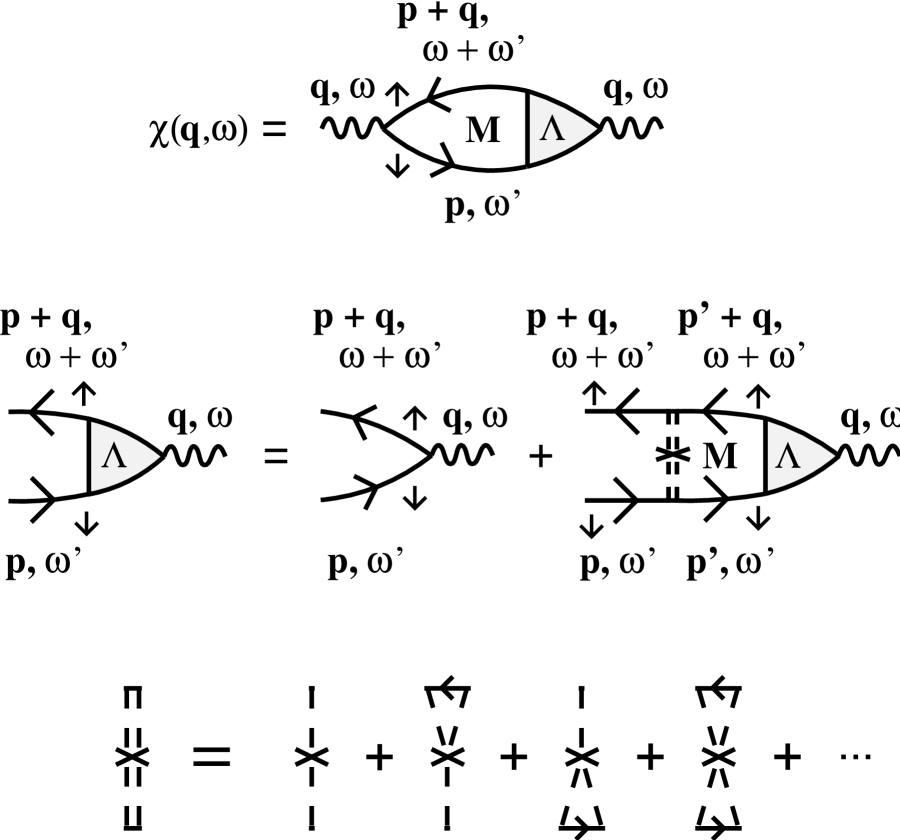
FIG. 6.: Diagrammatic representation of the vertex corrections to the spin susceptibility in the normal state due to impurity scattering in the non-crossing or dilute limit.

The vertex corrected susceptibility bubble $\chi({\bf q},i\omega_{m})$ is given by a particle-hole bubble $M({\bf q},i\omega_{m},{i\omega_{n}})$ with a simple vertex at one end and a dressed vertex $\Lambda({\bf q},i\omega_{m},{i\omega_{n}})$ at the other end. In the normal state this may be written as

$$\chi({\bf q},i\omega_{m})=T\sum_{n}~{}M({\bf q},i\omega_{m},{i\omega_{n}})~{}\Lambda({\bf q},i\omega_{m},{i\omega_{n}}),$$ (23)

where

$$M({\bf q},i\omega_{m},{i\omega_{n}})=-\int{d^{2}p\over(2\pi)^{2}}~{}G({\bf p}+{\bf q},{i\omega_{m}}+{i\omega_{n}})~{}G({\bf p},{i\omega_{n}}).$$ (24)

The dressed vertex is given by the sum of a series of ladder diagrams where impurity scattering lines [represented by $\Gamma({i\omega_{m}},{i\omega_{n}})$] are allowed to connect the particle and hole lines:

$$\Lambda({\bf q},i\omega_{m},{i\omega_{n}})=1+\Gamma({i\omega_{m}},{i\omega_{n}})~{}M({\bf q},i\omega_{m},{i\omega_{n}})~{}\Lambda({\bf q},i\omega_{m},{i\omega_{n}}).$$ (25)

Equations (23) and (25) are easily rearranged to yield

$$\chi({\bf q},i\omega_{m})=T\sum_{n}~{}{M({\bf q},i\omega_{m},{i\omega_{n}})\over 1-\Gamma({i\omega_{m}},{i\omega_{n}})~{}M({\bf q},i\omega_{m},{i\omega_{n}})}.$$ (26)

Since the impurity scattering lines include any number of multiple scattering events, they are given simply by a product of two of the t-matrices used in the self energy calculation:

$$\Gamma({i\omega_{m}},{i\omega_{n}})=-{n_{i}\over[\pi N(0)]^{2}}~{}T_{0}({i\omega_{m}}+{i\omega_{n}})~{}T_{0}({i\omega_{n}}).$$ (27)

Since we are considering only the unitary scattering limit, i.e. $c=0$, the $T_{3}$ component of the scattering t-matrix vanishes. Thus $\Gamma({i\omega_{m}},{i\omega_{n}})$ contains contributions from $T_{0}$ only.

A complication which arises in the superconducting state is that the dressed vertex cannot be represented as a simple scalar function. Since the electron and hole propagators must be represented by both normal and anomalous propagators to account for electrons scattering into and out of the superconducting condensate, the dressed vertex is represented by a four component vector which accounts for all possible combinations of electron and hole lines going into and out of the vertex, as shown in Fig. 7.

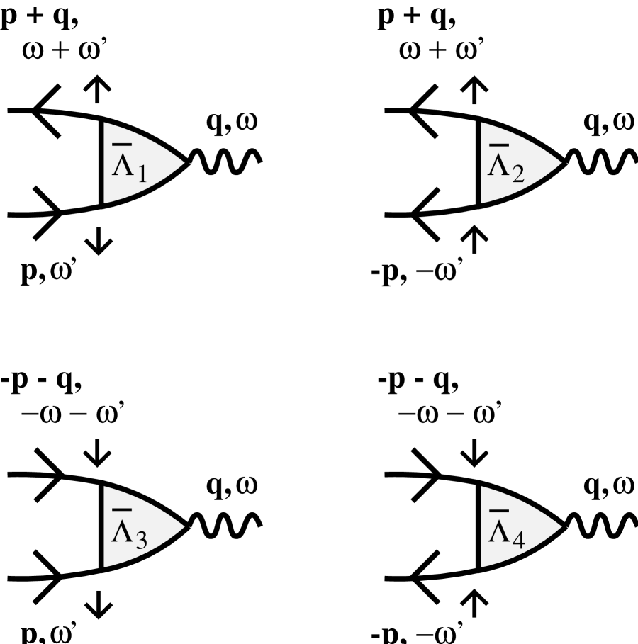
FIG. 7.: Components of the dressed vertex in the superconducting state.

The equations for the vertex corrected spin susceptibility

$$\underline{\chi}({\bf q},i\omega_{m})=T\sum_{n}~{}\underline{M}({\bf q},i\omega_{m},{i\omega_{n}})~{}\overline{\Lambda}({\bf q},i\omega_{m},{i\omega_{n}})$$ (28)

and for the dressed vertex

$$\overline{\Lambda}({\bf q},i\omega_{m},{i\omega_{n}})=\overline{1}+\Gamma({i\omega_{m}},{i\omega_{n}})~{}\underline{M}({\bf q},i\omega_{m},{i\omega_{n}})~{}\overline{\Lambda}({\bf q},i\omega_{m},{i\omega_{n}})$$ (29)

then become matrix equations where the vertices are 4-component vectors (overscored symbols) and the particle-hole bubbles are represented by 4x4 matrices (underscored symbols). Equation (29) represents four separate equations, one for each component of $\overline{\Lambda}({\bf q},i\omega_{m},{i\omega_{n}})$. The diagrammatic representation of the first of these is shown in Fig. 8. The diagrammatic representations for the other three components are similar. The diagrams corresponding to the components of the matrix $\underline{M}({\bf q},i\omega_{m},{i\omega_{n}})$ are shown schematically in Fig. 9. Explicitly, the components of $\underline{M}({\bf q},i\omega_{m},{i\omega_{n}})$, which is symmetric, are

$$\underline{M}_{11}({\bf q},{i\omega_{m}},{i\omega_{n}}) =-\underline{M}_{22}({\bf q},{i\omega_{m}}+2{i\omega_{n}},-{i\omega_{n}})=-\underline{M}_{33}({\bf q},-{i\omega_{m}}-2{i\omega_{n}},{i\omega_{n}})$$ (32)

$$=\underline{M}_{44}({\bf q},-{i\omega_{m}},-{i\omega_{n}})=-\int{d^{2}p\over(2\pi)^{2}}~{}G({\bf p}+{\bf q},{i\omega_{m}}+{i\omega_{n}})~{}G({\bf p},{i\omega_{n}}),$$

$$\underline{M}_{12}({\bf q},{i\omega_{m}},{i\omega_{n}}) =\underline{M}_{13}({\bf q},-{i\omega_{m}},{i\omega_{m}}+{i\omega_{n}})=-\underline{M}_{24}({\bf q},{i\omega_{m}}+2{i\omega_{n}},-{i\omega_{m}}-{i\omega_{n}})$$ (35)

$$=-\underline{M}_{34}({\bf q},-{i\omega_{m}}-2{i\omega_{n}},{i\omega_{n}})=\int{d^{2}p\over(2\pi)^{2}}~{}G({\bf p}+{\bf q},{i\omega_{m}}+{i\omega_{n}})~{}F({\bf p},{i\omega_{n}}),$$

$$\underline{M}_{14}({\bf q},{i\omega_{m}},{i\omega_{n}}) =\underline{M}_{23}({\bf q},i\omega_{m},{i\omega_{n}})=-\int{d^{2}p\over(2\pi)^{2}}~{}F({\bf p}+{\bf q},{i\omega_{m}}+{i\omega_{n}})~{}F({\bf p},{i\omega_{n}}).$$ (37)

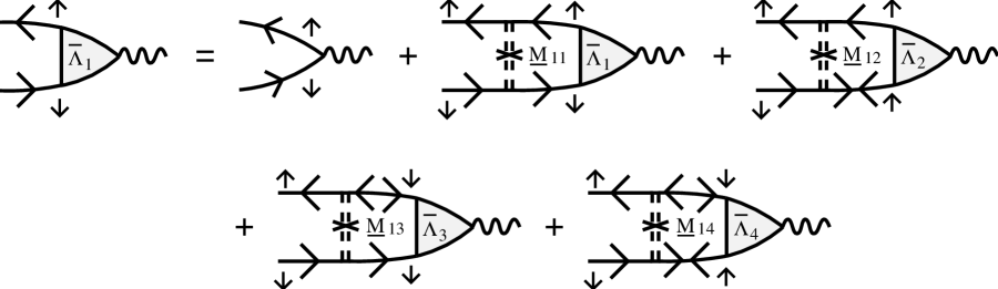
FIG. 8.: Diagrammatic representation of the first component of the matrix equation, Eq. (29), for the dressed vertex in the superconducting state.

FIG. 9.: Schematic representation of the diagrams corresponding to the components of the matrix $\underline{M}({\bf q},i\omega_{m},{i\omega_{n}})$.

Just as for the normal state, Eqs. (28) and (29) may be rearranged, yielding

$$\underline{\chi}({\bf q},i\omega_{m})=T\sum_{n}~{}\underline{M}({\bf q},i\omega_{m},{i\omega_{n}})~{}[\underline{1}-\Gamma({i\omega_{m}},{i\omega_{n}})~{}\underline{M}({\bf q},i\omega_{m},{i\omega_{n}})]^{-1}.$$ (38)

As mentioned previously, the vertex representing magnetic neutron scattering connects only electrons of opposite spin. Thus to recover the quantity corresponding to the spin susceptibility measured by magnetic neutron scattering we must now add the components of $\underline{\chi}({\bf q},i\omega_{m})$ which correspond to diagrams which begin and end with opposite spin electron lines:

$$\chi({\bf q},i\omega_{m})=\underline{\chi}_{11}({\bf q},i\omega_{m})+\underline{\chi}_{41}({\bf q},i\omega_{m}).$$ (39)

To avoid double counting, $\underline{\chi}_{14}({\bf q},i\omega_{m})$ and $\underline{\chi}_{44}({\bf q},i\omega_{m})$ are not included.

Figure 10 shows $\chi^{\prime\prime}({\bf q},\omega)$ calculated with and without impurity vertex corrections.

FIG. 10.: $\chi^{\prime\prime}({\bf q},\omega)$ with and without the inclusion of impurity vertex corrections as a function of momentum. The curves represent the following: (solid) normal state, vertex corrected; (short dashes) normal state, no vertex corrections; (long dashes) superconducting state, vertex corrected; (dotted) superconducting state, no vertex corrections.

Here $\chi({\bf q},i\omega_{m})$ has been calculated for imaginary frequencies. The real frequency results were then obtained by analytic continuation using Padé approximants.[11] In the normal state the vertex corrections do not have a dramatic effect on the zone edge peak structures. There is a noticeable decrease in $\chi^{\prime\prime}({\bf q},\omega)$ along the zone diagonal. In the superconducting state the impurity vertex corrections lead to a further enhancement of the peaks at the zone edge positions. These peaks are now comparable in size to those in the normal state.

III Coulomb interaction effects

In addition to impurity scattering, it is important to take into account the effects of the spin correlations produced by the Coulomb interaction. These have been shown to play an essential role in calculations of both the normal and the superconducting NMR responses.[5] Furthermore, as noted in the introduction, Coulomb spin susceptibility enhancement effects have been shown to maintain the neutron scattering peaks at their normal state positions along the Brillouin zone edge.[6, 7] Just as in the NMR and neutron scattering studies, we treat the Coulomb interaction within an RPA approximation in which

$$\chi({\bf q},\omega)={\chi_{0}({\bf q},\omega)\over{1-\overline{U}\chi_{0}({\bf q},\omega)}}.$$ (40)

Here, however, $\chi_{0}({\bf q},\omega)$ is the spin susceptibility in the presence of impurities discussed in Sec.II. The interaction $\overline{U}$ represents a renormalized Coulomb interaction.[12] Figure 11 shows $\chi^{\prime\prime}({\bf q},\omega)$ calculated for $U=2t$.

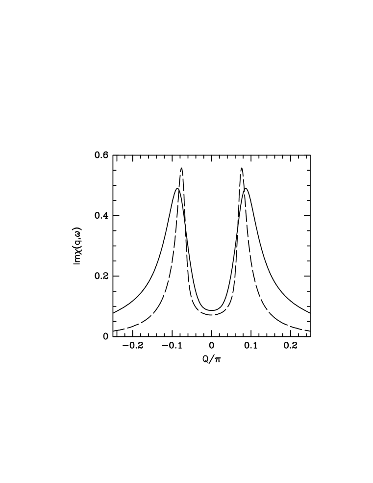
FIG. 11.: $\chi^{\prime\prime}({\bf q},\omega)$ with Coulomb enhancement effects included in the normal (solid line) and superconducting states (dashed line) as a function of momentum.

The Coulomb interaction enhances the normal state peak height by close to a factor of 60. This results in peak heights for the model which are of the same order of magnitude as the spin susceptibility peak heights reported by Mason and co-workers.[1, 13, 14]

As was mentioned in Sec. II, the Coulomb interaction also gives rise to dynamic lifetime effects through spin-fluctuation scattering. Previous calculations[15] have shown that scattering of electrons by spin fluctuations leads to the right order of magnitude for the quasiparticle relaxation rate in the normal state of the cuprates, i.e., $\tau^{-1}(T_{c})\sim T_{c}$. In the superconducting state, however, the gap in the electron excitation spectrum leads to a suppression of the low energy part of the spin fluctuation spectral weight and therefore to a suppression of the spin fluctuation scattering contribution to the quasiparticle relaxation rate.[16] Previous calculations[17] for a model system similar to the one used here have shown that for $T=0.1T_{c}$ and quasiparticle frequencies of order the temperature the quasiparticle relaxation rate due to spin fluctuation scattering is suppressed by several orders of magnitude compared to the value at $T_{c}$. For higher frequencies, such as those used in the experiments of Mason and co-workers, this relaxation rate is still small compared to the impurity scattering rate for the concentration of impurities we have considered here.[14] Thus the impurity scattering represents the dominant lifetime effect in the superconducting state results discussed here. In the normal state, on the other hand, the lifetime is determined by inelastic spin-fluctuation scattering. However, in the normal state, lifetime effects lead only to small changes in peak structure of $\chi^{\prime\prime}({\bf q},\omega)$, as shown in Fig. 5.

In order to directly compare the calculation including Coulomb enhancement effects to the experimental results we must average $\chi^{\prime\prime}({\bf q},\omega)$ over a region of momentum space comparable to the experimental resolution. Figure 12 shows $\chi^{\prime\prime}({\bf q},\omega)$ averaged over a region in momentum space with dimensions $0.04\pi$ by $0.12\pi$, the larger dimension being perpendicular to the momentum scan direction.

FIG. 12.: Momentum averaged $\chi^{\prime\prime}({\bf q},\omega)$ in the normal (solid line) and superconducting states (dashed line) as a function of momentum.

These results show some qualitative agreement with the experimental data. At the zone edge and zone diagonal the magnitude of $\chi^{\prime\prime}({\bf q},\omega)$ is reduced by a factor of about one half in the superconducting state compared to the normal state. This reduction is, however, not quite isotropic. The zone edge peak structures are noticeably narrower in the superconducting state compared to the normal state.

IV Conclusions

We have calculated the spin susceptibility at and below $T_{c}$ for a model $d_{x^{2}-y^{2}}$–wave superconductor with resonant impurity scattering and Coulomb correlations. Impurity scattering effects, including vertex corrections, act to restore the zone edge peaks in the spin susceptibility which are otherwise suppressed by a $d$–wave superconducting gap. The predicted amount of suppression of the spin susceptibility in the superconducting state compared to the normal state is in qualitative agreement with the experimental results in that the predicted neutron scattering intensity at the zone edge and along the diagonal is suppressed by about one half in the superconducting state compared to the normal state. The peak structure predicted by this model differs from the experimental results in that the peaks narrow appreciably at low temperatures compared to the normal state.

- [1] T. E. Mason, G. Aeppli, S. M. Hayden, A. P. Ramirez, and H. A. Mook, Phys. Rev. Lett. 71, 919 (1993).
- [2] J. P. Lu, Phys. Rev. Lett. 68, 125 (1992).
- [3] Y. Zha, K. Levin, and Q. Si, Phys. Rev. B 47, 9124 (1993).
- [4] P. J. Hirschfeld and N. Goldenfeld, Phys. Rev. B 48, 4219 (1993); W. N. Hardy, D. A. Bonn, D. C. Morgan, R. Liang, and K. Zhang, Phys. Rev. Lett. 70, 3999 (1993).
- [5] K. Ishida, Y. Kitaoka, N. Ogata, T. Kamino, K. Asayama, J. R. Cooper, and N. Athanassopoulou, J. Phys. Soc. Jpn. 62, 2803 (1993); T. Hotta, ibid. 62, 274 (1993).
- [6] N. Bulut and D. J. Scalapino, Phys. Rev. B 47, 3419 (1993).
- [7] K. Maki and H. Won, Phys. Rev. Lett. 72, 1758 (1994).
- [8] P. B. Littlewood, J. Zaanen, G. Aeppli, and H. Monien, Phys. Rev. B 48, 487 (1993).
- [9] P. J. Hirschfeld, P. Wölfle, and D. Einzel, Phys. Rev. B 37, 83 (1988).
- [10] Note that to obtain the above equations for the impurity scattering rate we must assume both that the average of the superconducting gap over the Fermi surface vanishes and that the system has particle-hole symmetry.[9] This second assumption does not hold for the tight-binding band used in our model. However, we are only interested in the impurity scattering at temperatures and frequencies small compared to the superconducting gap . At such a small energy scale particle-hole symmetry is approximately obeyed, and corrections due to the lack of such symmetry will be small.
- [11] H. J. Vidberg and J. W. Serene, J. Low Temp. Phys. 29, 179 (1977); G .A. Baker Jr., Essentials of Padé Approximants (Academic, New York, 1975), Chap. 8.
- [12] N. Bulut, D. J. Scalapino, and S. R. White, Phys. Rev. B 47, 2742 (1993).
- [13] T. E. Mason, G. Aeppli, S. M. Hayden, A. P. Ramirez, and H. A. Mook (unpublished).
- [14] S. M. Quinlan, Ph.D. thesis, University of California, Santa Barbara, 1994.
- [15] P. Monthoux and D. Pines, Phys. Rev. B 49, 4261 (1994); T. Moriya, Y. Takahashi, and K. Ueda, J. Phys. Soc. Jpn. 59, 2905 (1990).
- [16] M. C. Nuss, P. M. Mankiewich, M. L. O’Malley, E. H. Westerwick, and P. B. Littlewood, Phys. Rev. Lett. 66, 3305 (1991).
- [17] S. M. Quinlan, D. J. Scalapino, and N. Bulut, Phys. Rev. B 49, 1470 (1994).