NMR Spectroscopy and the Crystal-Field Interaction in Holmium Trifluoride

A thesis submitted to the University of Manchester
for the degree of Doctor of Philosophy
in the Faculty of Science

Simeon Mark Warner
Department of Physics
April 1994

Contents

• toc

Abstract

The work to be described falls into three parts: (1) the design, construction and testing of a continuous-wave (CW) microwave NMR spectrometer; (2) an NMR study of the hyperfine splittings of holmium trifluoride, supplemented by magnetometry; and (3) theoretical analysis.

(1) The computer-controlled CW spectrometer was designed to supplement the Manchester pulsed microwave spectrometer in situations where rapid nuclear relaxation makes spin-echo spectroscopy difficult. Its operating range is 4–8 GHz. Resonator designs and modulation strategies will be discussed in the light of practical experience.

(2) Both CW and pulsed NMR have been used to study the field dependence of the hyperfine splittings of ¹⁶⁵Ho in HoF₃ and, as a dilute substituent, in YF₃. The low site symmetry results in a singlet crystal-field ground state for the Ho³⁺ ion, giving Van Vleck paramagnetism and enhanced nuclear magnetism at low temperatures. The measurements were made at temperatures in the range 1.5 to 4.2 K and in fields of up to 8 T. This work has revealed, for the first time, distinct spectra from the two subtly inequivalent rare-earth sites in the orthorhombic unit cell. Because of the non-colinear spin structure of HoF₃, the NMR and magnetometry measurements give independent and complimentary information about the ionic moments.

(3) The measured hyperfine splittings have been interpreted in terms of a 15-parameter crystal-field Hamiltonian appropriate to the $C_{1h}$ site symmetry. This work has entailed a substantial effort to clarify the notational confusion that exists in the literature. A computer program has been developed to automate conversion between notational conventions prior to diagonalization of the 136-dimensional electronic-nuclear Hamiltonian comprising the Zeeman, crystal-field and hyperfine interactions.

Our experimental results are in fair agreement with calculated magnetizations and hyperfine splittings based on crystal-field parameters derived from high-resolution optical spectroscopy. However, there are discrepancies which suggest the need for refinement of the crystal-field parameters. The existing parameters predict that the hyperfine splitting will vary dramatically with the orientation of the applied field but technical difficulties have prevented an investigation of this effect during the time scale of the present work.

Declaration

No portion of the work referred to in this thesis has been submitted in support of an application for another degree or qualification of this or any other university or other institute of learning.

Chapter 1 Introduction

The rare-earth elements and compounds containing them exhibit a wide variety of magnetic properties. Moreover, they have proved amenable to detailed study. Since the 1950s, when rare earths of reasonable purity became available, they have been intensively studied revealing not only many physically interesting phenomena, but also industrially useful materials. In this work we shall be concerned solely with insulating rare-earth compounds.

Table 1.1 shows the rare-earth or lanthanide group of the periodic table. The elements La to Eu are often called light rare earths and the elements Gd to Lu heavy rare earths. Yttrium is not a rare earth but is often given honorary rare earth status because it is chemically very similar. Most rare earths are triply ionised in solids; in this state only the $4f$ shell is partially filled. The radius of the $4f$ shell is several times smaller than typical interionic separations and the $4f$ electrons do not take part in chemical bonding. However, the $4f$ electrons have large angular momentum and dominate the magnetic properties of the ion.

57	58	59	60	61	62	63	64	65	66	67	68	69	70	71
La	Ce	Pr	Nd	Pm	Sm	Eu	Gd	Tb	Dy	Ho	Er	Tm	Yb	Lu

Table 1.1: The rare-earth elements.

The ‘outer electrons’ shield the $4f$ shell from its surroundings and the rare earths retain their free-ion character in solids to a high degree. As in the free ions, the $L$-$S$ or Russell-Saunders coupling scheme is a good approximation in solids. In general $L$, $S$ and $J$ are fairly good quantum numbers, and spin-orbit coupling gives highest $J$ as ground state for heavy rare earths.

1.1 Rare-earth magnetism

Rare-earth ions maintain their free-ion character in solids more closely then any other elements. To a good first approximation the crystal-field and Zeeman interactions leave the spin-orbit coupling intact; their principal effect is to lift the degeneracy of the $J$-manifolds.

Bethe’s seminal paper [7] showed that open-shell energy levels of an ion in a crystalline environment were associated with the symmetry of the site. He also considered the terms required to describe the interaction of the ion with its environment for different point group symmetries. This was the birth of crystal-field theory. Condon and Shortley [25] provided the basic techniques for a perturbation approach to crystal-field calculations. Then, in a classic series of papers, Racah [60, 61, 62] developed the powerful tensor operator notation and discussed calculation of the matrix elements. All of this work was based in group theory and on the work of Wigner, especially the Wigner-Eckart theorem [25].

From the original well-structured works of Bethe, Condon and Shortly, and Racah, crystal-field theory has been developed in an ad hoc manner. Abragam and Bleaney [1] note that it is unfortunate that the pioneer work of Stevens [74] and of Elliott and Stevens [33, 35, 34] was not expressed in the more rational formalism of Racah. However, Elliott and Stevens were successful in accounting, in detail, for paramagnetic resonance data on some rare-earth salts. In appendix A we review parameter conventions for crystal fields and the inter-relationships between them. Having identified the more coherent conventions, appendix B describes the transformation of parameters under coordinate rotation. This is useful in helping to relate the crystal fields of inequivalent ions in sites with surroundings related by rotation.

Ab initio calculation of crystal-field and free-ion parameters remains intractable, so the parameters must be determined experimentally. Data from NMR spectroscopy alone are not usually sufficient to determine crystal-field parameters; the parameters are usually obtained from optical or neutron spectroscopy. Crystal-field parameters so obtained provide a basis for the detailed analysis of NMR data. For example Carboni [20] used the computed ground state of Ho³⁺ in Ho(OH)₃ to include $J$-mixing in his analysis of NMR data and to refine the hyperfine parameters of Ho³⁺.

1.2 Rare-earth trifluorides

The rare earths form many fluorides, the structures and chemisty of which are reviewed by Greis and Haschke [38]. Industrially, the fluorides are used for the manufacture of arc carbons with well balanced light emission. Of these the anhydrous trifluorides have been most intensively studied. They are chemically stable in air and moisture at room temperature. As a result, rare-earth trifluorides have proved a useful intermediate in the preparation of high-purity rare-earth metals [75]. Pure metals are produced from the trifluorides by reduction with calcium metal in an inert atmosphere.

In this work we consider only the trifluorides that are isostructural with YF₃: in particular HoF₃ and YF₃. There have been several X-ray and neutron structure determinations for rare-earth trifluorides which are in fairly good agreement. There is no argument about the $C_{1h}$ site symmetry of the rare-earth ions. Using just the structural and symmetry data we deduce that there are two inequivalent rare-earth sites in the unit cell (chapter 5).

HoF₃ is a Van Vleck paramagnet with strongly enhanced nuclear magnetism. It orders antiferromagnetically at $T_{N}=0.53$ K [11], due mainly to the dipole-dipole interaction. The ordered state has been studied by neutron diffraction [13]. Of the other trifluorides, only TbF₃ has been studied in the ordered state [41]. Like HoF₃, TbF₃ orders antiferromagnetically, but at a considerably higher temperature: $T_{N}=3.95$ K [41]. In this work we have used NMR to study the field dependence of the hyperfine splittings of Ho³⁺ in paramagnetic HoF₃, and as a dilute substituent in YF₃. We have also measured the magnetization in fields of up to 10 T along the principal crystallographic directions. The experimental data are compared with calculations based on crystal-field parameters derived from optical spectroscopy.

1.3 CW NMR

Rare-earth NMR is usually performed by pulsed techinques, principally spin-echo. Whilst pulsed NMR techniques have become extremely sophisticated for chemical systems, NMR of rare-earths is constrained by the technical difficulties associated with the very high frequencies (up to 7 GHz) and fast relaxation. As part of this work I have built a new continuous-wave (CW) microwave spectrometer. Chapter 3 discusses the CW technique and compares it with pulsed techniques. Various detection strategies and sample-cell designs are considered. Chapter 4 describes the new spectrometer and how it has been used. The majority of the NMR data in this thesis were taken using the CW spectrometer; the rest were taken using the Manchester pulsed spectrometer [21, 49].

The CW spectometer operates over the range 4–8 GHz, which has allowed study of the hyperfine interection of ¹⁶⁵Ho in HoF₃. It can also be used for studies of ¹⁴¹Pr. The microwave system is very simple and could fairly easily be modified to extend the operating range down to 2 GHz, giving access to the resonances of ¹⁵⁹Tb, ¹⁶⁹Tm and ¹⁷¹Yb.

Chapter 2 Theory

In order to understand the properties of rare-earth compounds we need to consider both the interactions within the rare-earth ion and the interactions of the ion with its surroundings. In atomic physics, interactions are traditionally arranged in order of descending strength and each is treated as a perturbation on the previous one. The perturbation approach has proved remarkably successful for rare-earth ions. The ground $LS$-terms of rare-earth ions are given, to a good first approximation, by Hund’s rule. In the heavy rare earths the spin-orbit coupling results in the ground $J$-manifold having maximum $J$. Whilst we adopt the perturbation approach to arrive at the ground $J$-manifold, the crystal-field, Zeeman and hyperfine interactions are treated together. This is unavoidable for the the electronic crystal-field and Zeeman interactions which may be of similar strengths. The hyperfine interaction is weak compared with the electronic interactions but cannot be treated as a perturbation when the electronic levels are degenerate, or nearly degenerate: see section 2.1.

The hyperfine interaction is of particular importance to this work as NMR is our principal experimental technique. Section 2.6 discusses hyperfine spectra on the basis of an effective nuclear Hamiltonian; typical parameter values are given. Discussion of NMR techniques is deferred to chapter 3. In this work we consider only insulators, for which the exchange interaction is very weak. The theory described is applicable to the majority of the heavy rare-earth ions, but we shall concentrate on the Ho³⁺ ion.

Data from bulk magnetization and low-temperature heat capacity measurements can be related to the ionic energy levels and eigenstates. Low-temperature heat capacity measurements are easiest to interpret for systems where we can use the approximation of a two-level system, i.e. where a low-lying first excited state is well separated from the next excited state. In section 2.7 we consider the Schottky anomaly in the two-level approximation. Section 2.8 relates the magnetization to the thermal average of the electronic angular momentum.

2.1 The Hamiltonian

The Hamiltonian for a rare-earth ion in a crystalline environment consists of free-ion, crystal-field, Zeeman and hyperfine terms. We treat the didole-dipole and exchange interactions in the molecular-field approximation by including an effective molecular field in the Zeeman term. In sections 2.1.1 and 2.1.2 we briefly describe the contributions to the Hamiltonian which determine the ground $J$-manifold in the $L$-$S$ coupling approximation.

We may write the total Hamiltonian as:

$${\cal H}={\cal H}_{0}+{\cal H}_{1}+{\cal H}_{so}+{\cal H}_{el}+{\cal H}_{h\!f},$$ (2.1)

where ${\cal H}_{0}$ is the central-field approximation to the Coulomb interaction; ${\cal H}_{1}$ is the non-central part of the Coulomb interaction; ${\cal H}_{so}$ is the spin-orbit interaction; ${\cal H}_{el}$ is the interaction of the electrons with their surroundings, both magnetic and electric; and ${\cal H}_{h\!f}$ is the hyperfine interaction.

For rare-earth ions it is usually a good approximation that

$${\cal H}_{0}\gg{\cal H}_{1}\gg{\cal H}_{so}\gg{\cal H}_{el}.$$ (2.2)

We shall consider the terms in sequence; each term as a perturbation on the previous one. The term ${\cal H}_{el}$ includes both the crystal-field and Zeeman interactions: ${\cal H}_{el}={\cal H}_{c\!f}+{\cal H}_{z}$. At high fields the strength of the Zeeman interaction can approach that of the crystal field, so they cannot be treated separately. The hyperfine interaction is much weaker than the crystal-field and Zeeman interactions and can usually be treated as a perturbation (${\cal H}_{el}\gg{\cal H}_{h\!f}$). However, this approximation can break down in the region of electronic level crossings. This situation has been investigated by Han [40].

With current computing power it is not necessary to treat the hyperfine interaction as a perturbation on ${\cal H}_{el}$; therefore we diagonalise ${\cal H}_{el}$ and ${\cal H}_{h\!f}$ together: see appendix C. The combined electronic-nuclear Hamiltonian is $(2I+1)(2J+1)$-dimensional.

2.1.1 Coulomb Hamiltonian, ${\cal H}_{0}+{\cal H}_{1}$

The dominant contribution to the Coulomb Hamiltonian may be reprsented by a central-field Hamiltonian ${\cal H}_{0}$ which determines the arrangements of electons in shells, the configurations. In the rare earths, all shells apart from the $4f$ are completely full or completely empty and so have no net angular momentum or magnetic moment. Omitting the labels of closed shells, the ground configuration of the holmium ion Ho³⁺ is $4f^{10}$. The first excited configuration of holmium is $>50000$ K above the ground configuration. There can be admixture of different configurations, usually referred to as the configuration interaction [64], but this effect is very small and we shall not consider it further. In this work we assume the $4f^{10}$ ground configuration of holmium.

The Coulomb repulsion ${\cal H}_{1}$ couples the individual electronic angular and orbital momenta such that $L$ and $S$ are good quantum numbers. This splits the configuration into non-degenerate $LS$-terms, a situation known as $L$-$S$ or Russell-Saunders coupling.

2.1.2 Spin-orbit coupling, ${\cal H}_{so}$

The principal effect of the spin-orbit interaction is to couple $L$ and $S$ to form a total angular momentum $J$, with $J$ as a good quantum number. Here we are assuming $L$-$S$ coupling which is a good approximation in rare-earths because ${\cal H}_{1}\gg{\cal H}_{so}$. Thus the spin-orbit interaction may be written as

$${\cal H}_{so}=\zeta{\mbox{\boldmath$L$}}.{\mbox{\boldmath$S$}},$$ (2.3)

where $\zeta$ is the coupling parameter. In Ho³⁺ the first excited manifold ${}^{5}I_{7}$ is $\approx 7500$ K above the ${}^{5}I_{8}$ ground manifold [29]. The spin-orbit coupling shifts the energies of the $LS$-terms slightly, and also mixes different $LS$-terms: see section 2.1.3.

In this work we use the $L$-$S$ states as the basis for electronic calculations. They are labelled $\mid\tau LSJM_{J}\rangle$, where $\tau$ is and extra index to identify different terms with the same $L$ and $S$. We use $M_{J}$ to denote the eigenvalues of $J_{z}$. In heavy rare-earth ions, the spin-orbit interaction is such that $L$ and $S$ couple to give the maximum possible $J=L+S$, and conversely for light rare-earths. The ground state of Ho³⁺ is ${}^{5}I_{8}$, i.e. $L=6$, $S=2$, $J=8$ and $M_{J}=-8\ldots 8$.

2.1.3 Intermediate coupling

Spin-orbit coupling admixes states of different $L$ and $S$ but with the same $J$. The effect of this is that $J$ is a much better quantum number than either $L$ or $S$. Although the $LS$-terms are well separated, the admixture is a significant effect and is usually allowed for by the use of modified operator-equivalent coefficients $\langle J\parallel\alpha_{k}\parallel J\rangle$ and Landé $g$-factors ${g_{\!{}_{J}}}$. The values of $\langle J\parallel\alpha_{k}\parallel J\rangle$ for the ground manifold of Ho³⁺ are modified by $\approx$8%, and this is known as intermediate coupling. Estimates for the operator-equivalent coefficients for some of the rare-earths are given by Dieke [28] and for Ho³⁺ by Rajnak and Krupke [63].

Carboni [20] discusses the admixture of $LS$-terms by the spin-orbit coupling. If we write the ground state $\mid\xi_{0}\rangle$ as linear combination of $L$-$S$ states (our chosen basis) then

$$\mid\xi_{0}\rangle=\sum_{i}a_{i}\mid L_{i}S_{i}J_{i}\rangle,$$ (2.4)

where the summation is over all $LSJ$-manifolds $i$. For Ho³⁺ in Y(OH)₃ and in LaCl₃ the ground state is

$$\mid\xi_{0}\rangle \approx 0.967\>^{5}\!I+0.116\>^{3}\!K_{1}-0.221\>^{3}\!K_{2}-0.031\>^{3}\!L-0.006\>^{3}\!M$$ (2.5)

$$+0.011\>^{1}\!L_{1}+0.033\>^{1}\!L_{2}.$$

For both compounds the Landé $g$-factor is ${g_{\!{}_{J}}}$ = 1.2417 with an uncertainty estimated at $\pm 0.00005$ [20]. This is about 0.7% smaller than the pure $L$-$S$ value of 1.25.

2.1.4 $J$-mixing

In the free ion, $J$ is a rigorously good quantum number if we ignore the hyperfine interaction. In general, the crystal-field and Zeeman interactions have matrix elements between different $J$-manifolds so $J$ ceases to be a good quantum number, an effect known as $J$-mixing. The splitting between the lower manifolds in heavy rare earths is much larger than in light rare earths, so $J$-mixing is less significant in the heavy rare earths. In holmium the ground and first excited manifolds are separated by $\approx 7500$ K [32]. With such a large separation we expect $J$ to remain a fairly good quantum number. In high precision studies $J$-mixing can be significant, see for example Carboni [20]. $J$-mixing has not been included in this work.

2.2 Crystal-field Hamiltonian, ${\cal H}_{c\!f}$

The crystal-field interaction is the interaction of the aspherical electronic charge distribution of the ion with the inhomogeneous electric field produced by the surrounding ions. Firstly, we make the approximation that the charges producing the crystal field do not overlap with the $4f$ electrons. Then Laplace’s equation, $\nabla^{2}V=0$, will hold for the potential experienced by the $4f$ electrons and we may expand the crystal-field interaction in terms of spherical harmonics, ${Y_{kq}(\theta,\varphi)}$:

$${\cal H}_{c\!f}=\sum_{i=1}^{n}\sum_{kq}(r_{i})^{k}A_{k}^{q}Y_{kq}(\theta_{i},\varphi_{i}).$$ (2.6)

where $(r_{i},\theta_{i},\varphi_{i})$ is the position of the $i^{th}$ electron and the $A_{k}^{q}$ are the coefficients of the expansion. The number of parameters in the expansion is limited by the requirements that $k$ must be even, and $k\leq 2l$. For $f$ electrons $l=3$, so at most 27 parameters are required: we need only the terms for $k=2,4,6$ and $q=-k\ldots k$.

In writing the expansion we have assumed a coordinate system $(r,\theta,\varphi)$ relating the ion to its surroundings. This choice of coordinate system will affect the parameters $A_{k}^{q}$ of the expansion and, possibly, the number required. The number of parameters required depends on the site symmetry in terms of the chosen coordinate system. This point is discussed in appendix A where the minimum number of parameters required for different site symmetries are given. At this stage we take the opportunity to define the crystal-field axes, shown in figure 2.1. Appendix B describes the transformation of crystal-field parameters corresponding to rotation of the coordinate system.

 

 

Figure 2.1: Definition of crystal-field axes.

Application of the Wigner-Eckart theorem allows equation 2.6 to be recast in terms of a set of angular momentum operators. Adopting the convention of Morrison and Leavitt [52] we may write the crystal-field Hamiltonian as

$${\cal H}_{c\!f}=\sum_{k=2,4,6}\sum_{q=-k\ldots k}M_{q}^{k}C_{q}^{k},$$ (2.7)

where the $M_{q}^{k}$ are parameters and the $C_{q}^{k}$ are tensor operators which may be written in terms of the components of $J$. The $M_{0}^{k}$ are real and the $M_{q}^{k}$ are complex for $q\neq 0$, also $M_{q}^{k}=(-1)^{q}M_{q}^{k\ast}$. The operators $C_{q}^{k}$ are given by $C_{q}^{k}=\langle J\parallel\alpha_{k}\parallel J\rangle T_{q}^{k}$, where the $T_{q}^{k}$ are listed in table A.6 and the $\langle J\parallel\alpha_{k}\parallel J\rangle$ are operator-equivalent coefficients. Values of $\langle J\parallel\alpha_{k}\parallel J\rangle$ for the ground manifold of Ho³⁺ are given in table 2.1 There are many other conventions for parametrizing the crystal field: see appendix A.

The principal effect of the crystal-field interaction is to lift some or all of the degeneracy in $M_{J}$. It can also cause some $J$-mixing (see section 2.1.4 above). The crystal-field model represents the independent interaction of equivalent electrons with an effective potential. In using it to fit experimental data, any other effects that may be expressed in this form will automatically be included. The principal component of the interaction comes from the electrostatic potential due to surrounding ions. However, other mechanisms can make significant contributions to an interaction of this form, eg., covalency and the configuration interaction [54].

2.3 Zeeman interaction

The Zeeman interaction is the interaction of the electronic moment with a magnetic field $B$. The Hamiltonian is

$${\cal H}_{z}={g_{\!{}_{J}}}\mu_{B}{\mbox{\boldmath$B$}}.{\mbox{\boldmath$J$}}$$ (2.8)

where ${g_{\!{}_{J}}}$ is the Landé $g$-factor. It is convenient to include all effective fields in $B$ and we write:

$${\mbox{\boldmath$B$}}={\mbox{\boldmath$B$}}_{app}+{\mbox{\boldmath$B$}}_{dip}+{\mbox{\boldmath$B$}}_{m},$$ (2.9)

where ${\mbox{\boldmath$B$}}_{app}$ is the applied field; ${\mbox{\boldmath$B$}}_{dip}$ is the dipolar field (see section 2.5); and ${\mbox{\boldmath$B$}}_{m}$ is the molecular field used to model the exchange interaction.

Following McCausland and Mackenzie [50] the exchange field is considered to interact with the projected spin ${\mbox{\boldmath$\sigma$}}=({g_{\!{}_{J}}}-1){\mbox{\boldmath$J$}}$. The projected spin is related to $J$ by a scaling factor so the interaction can be rewritten in terms of an equivalent molecular field:

$${\mbox{\boldmath$B$}}_{m}=\left(\frac{{g_{\!{}_{J}}}-1}{{g_{\!{}_{J}}}\mu_{B}}\right){\mbox{\boldmath$X$}},$$ (2.10)

where $X$ is the exchange field. It is hard to calculate the exchange field and ${\mbox{\boldmath$B$}}_{m}$ is usually treated as a parameter. The exchange interaction is much weaker in insulating materials than in metals where the conduction electrons interact with the ionic spins. The exchange field is considered by Bunbury et al [18] who, using the Scott’s data [70], conclude that $B_{m}\approx-B_{dip}/4$ in Ho(OH)₃.

2.4 Hyperfine interaction

In this section we follow the notation of McCausland and Mackenzie [50]. The hyperfine interaction may be split into dipolar and quadrupolar terms:

$${\cal H}_{h\!f}={\cal H}_{h\!f\!d}+{\cal H}_{h\!f\!q},$$ (2.11)

where ${\cal H}_{h\!f\!d}$ is the magnetic dipole Hamiltonian and ${\cal H}_{h\!f\!q}$ is the electric quadrupole Hamiltonian. There are higher order interactions but their effect is not significant in our measurements so they are neglected. Both the dipole and quadrupole terms have intra-ionic and extra-ionic components, and it is convenient to separate them:

$${\cal H}_{h\!f}={\cal H}_{h\!f\!d}^{\prime}+{\cal H}_{h\!f\!d}^{\prime\prime}+{\cal H}_{h\!f\!q}^{\prime}+{\cal H}_{h\!f\!q}^{\prime\prime},$$ (2.12)

where the intra-ionic terms are denoted by a single prime and extra-ionic terms by a double prime.

2.4.1 Dipolar hyperfine interaction

The intra-ionic part of the dipolar hyperfine interaction is given by

$${\cal H}_{h\!f\!d}^{\prime}=hA({\mbox{\boldmath$J$}}.{\mbox{\boldmath$I$}}),$$ (2.13)

where $A$ is the dipolar coupling coefficient expressed as a frequency, hence the inclusion of Planck’s constant $h$. For holmium $A$ has been deduced from EPR experiments by Bleaney [10] and refined by Carboni [20]. The dipolar and other hyperfine parameters for the rare-earth are tabulated by Han [40]. When the hyperfine interaction is considered as a perturbation on the electronic Hamiltonian it is customary to express the intra-ionic dipolar parameter as $a_{0}^{\prime}=AJ$ (see section 2.6).

The extra-ionic dipole interaction is the Zeeman interaction of the nuclear dipole moment with the magnetic field at the ion. It is thus analogous to equation 2.8:

$${\cal H}_{h\!f\!d}^{\prime\prime}={g_{\!{}_{I}}}\mu_{N}{\mbox{\boldmath$B$}}^{\prime\prime}.{\mbox{\boldmath$I$}},$$ (2.14)

where ${g_{\!{}_{I}}}$ is the Landé g-factor for the nucleus (see table 2.1). The magnetic field ${\mbox{\boldmath$B$}}^{\prime\prime}$ may be written as

$${\mbox{\boldmath$B$}}^{\prime\prime}={\mbox{\boldmath$B$}}_{app}+{\mbox{\boldmath$B$}}_{dip}$$ (2.15)

where ${\mbox{\boldmath$B$}}_{app}$ and ${\mbox{\boldmath$B$}}_{dip}$ are the applied and dipolar contributions respectively. In metals there is also a contribution from the conduction electrons; here we are concerned only with insulators.

2.4.2 Quadrupolar hyperfine interaction

The intra-ionic part of the quadrupolar hyperfine interaction is

$${\cal H}_{h\!f\!q}^{\prime}=hC\left[3({\mbox{\boldmath$J$}}.{\mbox{\boldmath$I$}})^{2}+\frac{2}{3}({\mbox{\boldmath$J$}}.{\mbox{\boldmath$I$}})-J(J+1)I(I+1)\right],$$ (2.16)

where $C$ is the quadrupole coupling coefficient in the notation of Bunbury at al [18], expressed as a frequency. When the hyperfine interaction is considered as a perturbation on the electronic Hamiltonian it is customary to write the intra-ionic quadrupolar parameter as $P_{0}^{\prime}=CJ(2J-1)$ (see section 2.6).

The extra-ionic quadrupolar interaction is the interaction of the nuclear quadrupole moment with the electric-field gradient at the nucleus. In this way it is analogous to the quadrupolar crystal-field interaction of the electrons. In the absence of direct information, the electric field gradient (EFG) at the nucleus can be estimated from the crystal-field parameters. First, the EFG ‘seen’ by the ion can be estimated from the crystal-field parameters using the electronic antishielding factor and the electronic quadrupole moment. Then, ‘crystal-field parameters’ for the nucleus can be estimated from the extra-ionic EFG using the nuclear antishielding factor and the nuclear quadrupole moment. Details of this procedure are given by Bunbury et al [18] for the $B^{2}_{0}$ term (using the crystal-field notation of Baker, Bleaney and Hayes [4]). Han [40] added $B_{2}^{2}$ to cope with orthorhombic symmetry.

Here, we present a more general approach which includes all quadrupolar terms so that the extra-ionic quadrupolar interaction may be expressed with arbitrary coordinate axes and for any site symmetry. We write the extra-ionic quadrupole interaction similarly to the crystal-field interaction:

$${\cal H}_{h\!f\!q}^{\prime\prime}=\sum_{q=-2\ldots 2}\overline{M}_{q}^{2}\overline{C}_{q}^{2},$$ (2.17)

where the $\overline{M}_{q}^{2}$ are the paremeters; and the $\overline{C}_{q}^{2}$ are tensor operators like the $C_{q}^{k}$ but in the components of $I$. Following the procedure of Bunbury et al [18] and of Han [40] we can determine the $\overline{M}_{q}^{2}$:

$$\overline{M}_{q}^{2}=\frac{Q_{I}}{Q_{J}}\frac{\gamma_{n}}{\gamma_{e}}M_{q}^{2},$$ (2.18)

where the $M_{q}^{k}$ are the crystal-field parameters (equation 2.7); $Q_{I}$ and $Q_{J}$ are defined below; $\gamma_{n}$ and $\gamma_{e}$ are the nuclear and electronic antishielding factors respectively, in the notation of Edmonds [31]. The operators $\overline{C}_{q}^{2}$ are

$$\overline{C}_{q}^{2}\hskip 4.35556pt = \mbox{\hskip 4.35556pt}\langle J\parallel\alpha_{2}\parallel J\rangle\frac{1}{2}[3I_{z}^{2}-I(I+1)]$$

$$\overline{C}_{\pm q}^{2} = \mp\langle J\parallel\alpha_{2}\parallel J\rangle\frac{\sqrt{6}}{4}[I_{z}I_{\pm}+I_{\pm}I_{z}]$$

$$\overline{C}_{\pm q}^{2} = \mbox{\hskip 4.35556pt}\langle J\parallel\alpha_{2}\parallel J\rangle\frac{\sqrt{6}}{4}I_{\pm}^{2}$$ (2.19)

where the $\langle J\parallel\alpha_{2}\parallel J\rangle$ are the operator-equivalent coefficients and $I_{\pm}=(I_{x}\pm I_{y})$ as usual. Putting these operators into equation 2.17 gives

$${\cal H}_{h\!f\!q}^{\prime\prime} = \frac{Q_{I}}{Q_{J}}\frac{\gamma_{n}}{\gamma_{e}}\langle J\parallel\alpha_{2}\parallel J\rangle\left\{M^{2}_{0}\frac{1}{2}[3I_{z}^{2}-I(I+1)]-M^{2}_{1}\frac{\sqrt{6}}{4}[I_{z}I_{+}+I_{+}I_{z}]+\right.$$ (2.20)

$$\left.\mbox{\hskip 36.135pt}M^{2}_{-1}\frac{\sqrt{6}}{4}[I_{z}I_{-}+I_{-}I_{z}]+M^{2}_{2}\frac{\sqrt{6}}{4}I_{+}^{2}+M^{2}_{-2}\frac{\sqrt{6}}{4}I_{-}^{2}\right\}.$$

We define $Q_{I}$ and $Q_{J}$ as

$$Q_{I}=\frac{Q_{n}}{I(2I-1)}\mbox{\hskip 28.45274pt and\hskip 28.45274pt}Q_{J}=\frac{Q_{e}}{J(2J-1)}.$$ (2.21)

For calculation we use just the single parameter $Q_{ext}$, where

$$Q_{ext}=\frac{Q_{I}}{Q_{J}}\frac{\gamma_{n}}{\gamma_{e}}.$$ (2.22)

It is commonly assumed that the antishielding factors are isotropic and there is no experimental evidence to the contrary. They are, however, host dependent.

The extra-ionic quadrupole interaction may alternatively be written in terms of parameters in the Baker, Bleaney and Hayes [4] notation (extended to complex parameters):

$${\cal H}_{h\!f\!q}^{\prime\prime} = \frac{Q_{I}}{Q_{J}}\frac{\gamma_{n}}{\gamma_{e}}\left\{B_{2}^{0}[3I_{z}^{2}-I(I+1)]+B_{2}^{1}\frac{1}{4}[I_{z}I_{+}+I_{+}I_{z}]+\right.$$ (2.23)

$$\left.\mbox{\hskip 72.26999pt}B_{2}^{-1}\frac{1}{4}[I_{z}I_{-}+I_{-}I_{z}]+B_{2}^{2}\frac{1}{2}I_{+}^{2}+B_{2}^{-2}\frac{1}{2}I_{-}^{2}\right\}.$$

In the case of orthorhombic symmetry, equation 2.23 reduces to the equation given by Han [40] (our $B_{2}^{2}=B_{2}^{-2}$ real, and equal to Han’s $B_{2}^{2}$). For details of parameter conventions for crystal-fields see appendix A.

2.5 Dipolar field

The dipolar field is the field at a particular site resulting from all the other dipoles in the sample. We restrict this discussion to a paramagnetic sample but otherwise follow McCausland and Mackenzie [50]. The dipolar field may be written as

$${\mbox{\boldmath$B$}}_{dip}=\sum_{i}\frac{\mu_{0}}{4\pi}\left[\frac{3({\mbox{\boldmath$\mu$}}_{i}.{\mbox{\boldmath$r$}}_{i}){\mbox{\boldmath$r$}}_{i}}{r_{i}^{5}}-\frac{{\mbox{\boldmath$\mu$}}_{i}}{r_{i}^{3}}\right],$$ (2.24)

where the summation is over all other dipole moments ${\mbox{\boldmath$\mu$}}_{i}$, at positions ${\mbox{\boldmath$r$}}_{i}$ relative to the site of interest. Clearly, it is not possible to compute such a sum over a macroscopic sample. The normal procedure is to split the dipolar field into three components:

$${\mbox{\boldmath$B$}}_{dip}={\mbox{\boldmath$B$}}_{int}+{\mbox{\boldmath$B$}}_{L}+{\mbox{\boldmath$B$}}_{dm},$$ (2.25)

where ${\mbox{\boldmath$B$}}_{int}$ is the field resulting from dipole moments in a sphere centred on the site of interest, the ‘Lorentz sphere’; ${\mbox{\boldmath$B$}}_{L}$ is the Lorentz field; and ${\mbox{\boldmath$B$}}_{dm}$ is the demagnetizing field due to the outer surface of the sample. ${\mbox{\boldmath$B$}}_{int}$ can be calculated from equation 2.24 and this is referred to as a dipole sum, see section 2.5.1. We make the approximation of uniform magnetization outside the sphere. In doing this we assume that effect on the dipolar field of the positions of individual dipole moments in the lattice is not significant outside the Lorentz sphere. A uniformly magnetized spherical shell has no field at its centre, ${\mbox{\boldmath$B$}}_{L}=-{\mbox{\boldmath$B$}}_{dm}$. Thus, the dipolar field at the centre of a macroscopic spherical sample may be calculated by considering a microscopic sphere: ${\mbox{\boldmath$B$}}_{dip}={\mbox{\boldmath$B$}}_{int}$ because ${\mbox{\boldmath$B$}}_{L}=-{\mbox{\boldmath$B$}}_{dm}$.

The power of the Lorentz sphere concept is in decoupling the effects of the local magnetization from the demagnetizing effects of the sample surface. We may write ${\mbox{\boldmath$B$}}_{L}$ and ${\mbox{\boldmath$B$}}_{dm}$ as

$${\mbox{\boldmath$B$}}_{L}=\mu_{0}\frac{1}{3}{\mbox{\boldmath$M$}}\mbox{\hskip 28.45274pt and\hskip 28.45274pt}{\mbox{\boldmath$B$}}_{dm}=-\mu_{0}{\sf N}\overline{{\mbox{\boldmath$M$}}},$$ (2.26)

where $M$ is the magnetization at the surface of the Lorentz sphere; $\sf N$ is the second-rank demagnetization tensor and $\overline{{\mbox{\boldmath$M$}}}$ is the average magnetization over the entire sample. In general, equation 2.26 is hard to apply. Only if the sample is an ellipsoid is the magnetization uniform througout the sample (and hence ${\mbox{\boldmath$M$}}=\overline{{\mbox{\boldmath$M$}}}$) and N independent of position. Osborn [56] tabulates demagnetization factors along the three axes of the general ellipsoid. Most magnetization measurements are interpreted by approximating the actual sample shape to an ellipsoid. The approximation is discussed by Cronemeyer [27]. In the special case of a sphere, $\sf N$ reduces to a scalar $N=\frac{1}{3}$. Akishin and Gaganov [2] consider the demagnetizing effects in cylindrical and rectangular box samples, and list values for the diagonal components of the demagnetization tensor for various geometries.

2.5.1 Dipole sum

The field $B$ due to a collection of dipole moments $\mu_{i}$ at a relative positions ${\mbox{\boldmath$r$}}_{i}$ is given by equation 2.24. By resolving $B$ into cartesian components we obtain the components of the dipolar field tensor: $B_{xx}$, $B_{yy}$, $B_{zz}$, $B_{xy}\equiv B_{yx}$, $B_{xz}\equiv B_{zx}$ and $B_{yz}\equiv B_{zy}$. $B_{xy}$ denotes the component of the field in direction $x$ resulting from moments in direction $y$.

If the dipole moments are all the same (${\mbox{\boldmath$\mu$}}={\mbox{\boldmath$\mu$}}_{i}$ for all $i$), then the diagonal components are

$$B_{xx}=\sum_{i}\frac{\mu_{0}\mu_{x}}{4\pi}\left(\frac{3x_{i}^{2}}{r_{i}^{5}}-\frac{1}{r_{i}^{3}}\right)\mbox{\hskip 28.45274pt and similarly for $B_{yy}$ and $B_{zz}$};$$ (2.27)

and the off-diagonal components are

$$B_{xy}=\sum_{i}\frac{\mu_{0}\mu_{y}}{4\pi}\frac{3x_{i}y_{i}}{r_{i}^{5}}\mbox{\hskip 28.45274pt and similarly for $B_{yz}$ and $B_{xz}$}.$$ (2.28)

A computer program has been written to compute the components of the dipolar field tensor for any arrangement of ions in a unit cell. The unit cell axes are each specified by a vector, and do not have to be orthogonal. Summations are performed over a sphere of given radius. The program is written in ANSI C, and on an IBM PC compatible computer (33 MHz ’486DX) the summation runs at $\approx$7000 ions/s. The calculation time increases linearly with the number of ions in the sum and hence as the radius cubed. For HoF₃ the sum was found to converge to $\approx$1% in 10 nm radius and to within 0.01% in 50 nm radius (percentage of the largest term). Calculation to 50 nm radius for HoF₃ corresponds to a sum over $\approx 10^{7}$ ions and is computed in less than half an hour.

2.6 Rare-earth NMR

This section outlines the relation of NMR to the energy levels of the ion. A careful and more detailed exposition of NMR in general is given by Slichter [72]; NMR in rare earths is considered by McCausland and Mackenzie [50]. Consider the Zeeman interaction of a nucleus with moment $\mu$ in a magnetic field $B$. We may write the Hamiltonian:

$${\cal H}=-\mu_{0}{\mbox{\boldmath$\mu$}}.{\mbox{\boldmath$B$}}.$$ (2.29)

This gives $2I+1$ equally spaced Zeeman levels: $E=-\mu_{0}{g_{\!{}_{I}}}\mu_{n}BM_{I}$ where $M_{I}=-I\ldots I$. An NMR experiment normally excites transitions between adjacent levels: the selection rule is $\Delta M_{I}=\pm 1$. In rare-earth ions the dominant contribution to the ‘field’ at the nucleus is the ‘effective hyperfine field’ due to the $4f$ electrons.

If we assume that the hyperfine interaction does not modify $J$ then equation 2.13 becomes

$${\cal H}_{h\!f\!d}^{\prime}\approx hA\langle{\mbox{\boldmath$J$}}\rangle.{\mbox{\boldmath$I$}}=\mu_{0}{g_{\!{}_{I}}}\mu_{n}{\mbox{\boldmath$B$}}_{e\!f\!f}.{\mbox{\boldmath$I$}},$$ (2.30)

where ${\mbox{\boldmath$B$}}_{e\!f\!f}=hA\langle{\mbox{\boldmath$J$}}\rangle/(\mu_{0}{g_{\!{}_{I}}}\mu_{n})$.

For a set of $(2I+1)$ evenly spaced energy levels there would be just a single NMR frequency. In practice the nuclear energy levels are not quite evenly spaced because of quadrupolar interaction. This results in $2I$ different NMR frequencies. The quadrupolar interaction is usually much weaker than the dipolar interaction resulting in a spectrum of $2I$ resonances where the separation of the resonances is a small fraction of their frequencies (see section 2.6.1). Unlike most NMR, in rare-earth NMR resolved quadrupole structure is the norm. Traditionally, an effective nuclear Hamiltonian is derived by treating ${\cal H}_{h\!f}$ as a perturbation on the electronic Hamiltonian ${\cal H}_{el}$ (section 2.6.1). Although we diagonalise the combined Hamiltonian for the electrons and nucleus directly, the perturbation results are instructive.

2.6.1 Effective nuclear Hamiltonian

By considering the hyperfine interaction as a perturbation on the electronic Hamiltonian an effective nuclear Hamiltonian is obtained:

$${\cal H}_{n}=a_{t}I_{z}+P_{t}\left(I_{z}^{2}-\frac{1}{3}I(I+1)\right)+wI_{z}^{3},$$ (2.31)

where the $z$ axis is along the direction of $\langle{\mbox{\boldmath$J$}}\rangle$ and off-diagonal quadrupolar terms have been neglected. They only have effect in second-order and it is expected to be small. The parameters $a_{t}$ and $P_{t}$ are combined intra- and extra-ionic parameters for the dipole and quadrupole interactions respectively. Thus, $a_{t}=a^{\prime}+a^{\prime\prime}$ and $P_{t}=P^{\prime}+P^{\prime\prime}$. The parameter $w$ is the pseudo-octupole term which arises from cross-coupling of the dipolar and quadrupolar terms when the latter is treated in second-order perturbation theory [50].

From eqaution 2.31, the transition frequencies for $\mid M_{I}\rangle\leftrightarrow\mid M_{I}-1\rangle$ are:

$$\nu_{M_{I},M_{I}-1}=a_{t}+(2M_{I}-1)p_{t}+(3M_{I}^{2}-3M_{I}+1)w,$$ (2.32)

where $(-I+1)\leq M_{I}\leq I$. The effect of $w$ is to create an asymmetry in the spectrum and also to shift the whole spectrum by $w/4$. The pseudo-octupole term is usually very small ($w<1$ MHz). The NMR spectrum of a fully polarized Ho³⁺ ion ($\langle{J_{z}}\rangle=J$) is shown in figure 2.2. To give an idea of the frequencies involved the parameters are taken as $a_{t}=a_{0}^{\prime}$, $P_{t}=P_{0}^{\prime}$ and $w=0$ (see table 2.1).

If NMR spectra are obtained in the frequency domain then this model is very convenient for interpretation. Each spectrum can be fitted to some lineshape function centred on frequencies given by equation 2.32 to obtain $a_{t}$, $P_{t}$ and $w$. NMR spectra taken by sweeping an applied field cannot be so easily interpreted because there is no simple relationship between the frequencies and the applied field. Each field corresponds to a different ionic Hamiltonian (${\cal H}_{el}+{\cal H}_{h\!f}$).

 

Ho³⁺, $I=7/2$, taking $a_{t}=a^{\prime}_{0}=6497$ MHz, $P_{t}=P^{\prime}_{0}=62.7$ MHz and $w=0$.

 

Figure 2.2: NMR spectrum for a Ho³⁺ ion.

 

¹⁶⁵Ho³⁺, ground manifold predominantly ${}^{5}I_{8}$
$J=8$, $I=\frac{7}{2}$
${g_{\!{}_{J}}}$ = 1.2417⁽²⁾, ${g_{\!{}_{I}}}$ = 1.151
Intra-ionic hyperfine paremeters:
$a_{0}^{\prime}$ = 6497 (8) MHz⁽¹⁾ $\Rightarrow$ A = 812.1 (10) MHz 6502 (6) MHz⁽²⁾ $\Rightarrow$ 812.8 (8) MHz $P_{0}^{\prime}$ = 62.7 (30) MHz⁽¹⁾ $\Rightarrow$ C = 0.523 (25) MHz
Radial averages for the $4f$ electrons⁽³⁾:
$\langle r^{-3}\rangle$ = $7.106{\times 10^{31}}$ m^-3 $\langle r^{2}\rangle$ = $2.085{\times 10^{-21}}$ m² $\langle r^{4}\rangle$ = $1.081{\times 10^{-41}}$ m⁴ $\langle r^{6}\rangle$ = $1.181{\times 10^{-61}}$ m⁶
Reduced matrix elements for the ground manifold:
Reduced matrix Russell-Saunders Intermediate element coupling⁽⁴⁾ coupling⁽⁵⁾ $\langle J\parallel\alpha_{2}\parallel J\rangle$ $-2.222{\times 10^{-3}}$ $-2.040{\times 10^{-3}}$ $\langle J\parallel\alpha_{4}\parallel J\rangle$ $-3.330{\times 10^{-5}}$ $-3.082{\times 10^{-5}}$ $\langle J\parallel\alpha_{6}\parallel J\rangle$ $-1.294{\times 10^{-6}}$ $-1.203{\times 10^{-6}}$
Nuclear and electronic quadrupole moments:
$Q_{n}$ = $3.51(2){\times 10^{-28}}$ m²⁽⁶⁾ $\Rightarrow$ $Q_{I}$ = $1.67(1){\times 10^{-29}}$ m² $Q_{e}$ = $5.104{\times 10^{-22}}$ m² $\Leftarrow$ $Q_{J}$ = $4.254{\times 10^{-24}}$ m²⁽⁷⁾
Ratio of nuclear to electronic antishielding factors:
$\gamma_{n}/\gamma_{e}$ = 149(15) ⁽⁶⁾ in holmium hydroxide. 246(10) ⁽²⁾ in holmium ethylsulphate. 254 ⁽⁸⁾ in holmium aluminium garnet.
¹   Bleaney [10].
²   Carboni [20].
³   Freeman and Desclaux [37]
⁴   Abragam and Bleaney [1].
⁵   Rajnak and Krupke [63].
⁶   Bunbury et al [17].
⁷   Calculated from the $\langle J\parallel\alpha_{2}\parallel J\rangle$ of ⁽⁵⁾ and the $\langle r^{2}\rangle$ of ⁽³⁾.
⁸   McMorrow [51].

 

Table 2.1: Electronic and hyperfine parameters for holmium.

2.7 Low temperature heat capacity

Heat capacity measurements in the helium temperature range can be dominated by the contribution from the electronic Schottky anomaly. In general, the electronic internal energy for a single ion $U_{el}$ is given by

$$U_{el}=\frac{1}{Z}\sum_{i=1}^{n}E_{i}e^{\frac{E_{i}}{kT}}$$ (2.33)

where $E_{i}$ are the electronic energy levels and $Z$; $T$ is the temperature; and $Z$ is the partition function,

$$Z=\sum_{i=1}^{n}e^{\frac{-E_{i}}{kT}}.$$ (2.34)

Note that we consider only insulating compounds so there is no conduction electron contribution. Differentiating with respect to $T$ at constant field gives the electronic Schottky heat capacity $C_{el}$,

$$C_{el}=\frac{k}{Z}\sum_{i=1}^{n}\frac{E_{i}}{kT}^{2}e^{\frac{E_{i}}{kT}}-\frac{k}{Z^{2}}\left\{\sum_{i=1}^{n}\frac{E_{i}}{kT}e^{\frac{E_{i}}{kT}}\right\}.$$ (2.35)

In systems where the ground state and first excited state are well separated from higher excited states the heat capacity at low temperatures may be approximated by a two level system. For two levels $E_{1}$ and $E_{2}$, and writing $\beta=\frac{E_{2}-E_{1}}{kT}$, equation 2.35 simplifies to

$$C_{el}=k\beta^{2}\frac{e^{\beta}}{(e^{\beta}+1)^{2}}.$$ (2.36)

Differentiating this expression to find the value of $\beta$ corresponding to the maximum in $C_{el}$ yields a transcendental equation in $\beta$. Numerical solution gives maximum in $C_{el}$ when $\beta=2.399\ldots$ $\Rightarrow(E_{2}-E_{1})\approx 2.399kT_{max}$.

The analysis of experimental data is not as simple as just finding the heat capacity maximum. Unfortunately, in the temperature range we are interested in (up to 20 K) the lattice heat capacity rises steeply. It is usually necessary to subtract the lattice heat capacity $C_{lat}\propto T^{3}$ before considering the electronic Schottky heat capacity. The electronic Schottky heat capacity varies quite slowly around the maximum so small gradients resulting from other contributions may shift the apparent peak significantly.

2.8 Bulk magnetization

Given a suitable model for the rare-earth ion that predicts the electronic energy levels it is possible to calculate the bulk magnetization.

$${\mbox{\boldmath$M$}}=\mu_{B}{g_{\!{}_{J}}}\sum_{i=1}^{n}<i\mid{\mbox{\boldmath$J$}}\mid i>\frac{e^{\frac{-E_{i}}{kT}}}{Z}$$ (2.37)

where the summation is over all populated states $i$. The $E_{i}$ are the energies of the states and $Z$ is the partition function (equation 2.34). Care must be taken if there are inequivalent sites in the unit cell as the individual moments may then differ in magnitude and direction. One of the more significant problems encountered when comparing predictions with experimental data is the effect of the shape of the sample on the demagnetizing field (see section 2.5).

Chapter 3 CW NMR

NMR was first observed by CW spectroscopy. However, when Hahn [39] discovered spin echoes, pulse techniques rapidly became the method of choice and CW NMR is now almost forgotten. In this chapter we argue a case for the use of CW NMR with some rare-earth systems. First, section 3.1 outlines some of the physical properties that affect NMR.

Rare-earth NMR is technically difficult, principally because of the large hyperfine splittings which give NMR frequencies of up to 7 GHz. This is often compounded by fast relaxation rates which mean that fast pulse sequences are required for pulsed NMR. This, in turn, requires short, high power pulses. The Manchester pulsed spectrometer [21, 49] provides up to 200 W of microwave power in pulses as short as 30 ns with rise and fall times of 5 ns. In spite of technical difficulties, pulsed NMR has been very successful in studying the hyperfine splittings of rare-earth compounds. However, for some systems fast relaxation can be a crippling problem. The sensitivity of CW NMR does not suffer from fast relaxation as badly as pulsed NMR. CW and pulsed NMR techniques are compared in section 3.2.

Section 3.3 goes on to discuss the design of a CW NMR spectrometer. A peculiarity of NMR as used to study magnetism, as opposed to chemical structure, is that we often work in regimes where the relationship between the magnetization and the applied field is extremely non-linear. The intra-ionic dipolar interaction is the dominant contribution to the hyperfine splitting, so the NMR frequencies are roughly proportional to the electronic moment. Hence the relationship between the NMR frequencies and the applied field is often extremely non-linear. Partial saturation of the electronic magnetism is the norm and in extreme cases such as ferromagnetic materials the magnetization may respond only very weakly to applied fields. Line widths in rare-earth NMR vary from a few MHz to hundreds of MHz. Given the relationship between the ionic moment $\langle\mu\rangle$ and the applied field $B$ for a given system, we can translate the line width in frequency, at any given field, into the corresponding line width in field. Figure 3.1 illustrates this relationship. Typical values of the line width in field range from $<0.1$ T to $\approx 1$ T, and the line width obviously increases as the differential susceptibility falls with saturation. This tends to make the NMR frequency insensitive to changes in the applied field at high fields.

 

 

Figure 3.1: Graph illustrating a typical relationship between the line width in frequency $\Delta\omega$ and the corresponding line width in field $\Delta B$.

3.1 Spin dynamics and nuclear susceptibility

This section outlines some of the factors that affect the design of an NMR experiment on rare-earth systems. Slichter [72] gives a much more detailed description of NMR principles and techniques. We note that most of the common ‘chemical NMR’ techniques are unsuitable for rare-earth systems. This is principally because of the much faster relaxation rates and higher NMR frequencies encountered in rare-earth systems.

In general we perform NMR on system of nuclear spins that are coupled the each other and to the lattice. The lattice acts as a thermal resorvoir and the lattice temperature determines the equilibrium populations of the nuclear levels. If the populations are temporarily disturbed, by NMR for example, they will then relax back to their equilibrium values exponentially with a characteristic time $T_{1}$, the spin-lattice relaxation time. This relaxation time will impart a homogeneous line width to the resonance, with a Lorentzian line shape:

$$g_{1}(\omega)=\frac{T_{1}}{\pi(1+T_{1}^{2}(\omega-\omega_{0})^{2})},$$ (3.1)

where $\omega_{0}$ is the resonance frequency. However, spin-lattice relaxation is not usually the dominant contribution to the homgeneous line width. In rare-earths $T_{1}$ typically ranges from $\approx 10$ $\mu$s to $\approx 10$ ms at liquid-helium temperatures. Spin-lattice relaxation is intimately linked with saturation of NMR: see section 3.1.1.

Spin-spin relaxation is usually the dominant contribution to the lifetime of the individual nuclear spin eigenstates, and hence to the homogeneous line width: $\Delta\omega_{h}\approx\frac{2}{T_{1}}+\frac{2}{T_{2}}\approx\frac{2}{T_{2}}$, where $T_{2}$ is the spin-spin relaxation time. In general the line shape is not Lorentzian (often it is more closely Gaussian) so the definition of $T_{2}$ is not straightforward. However, for most of this chapter we assume exponential relaxation and hence a Lorentzian line shape, for which $T_{2}$ is simply defined (cf. $T_{1}$ and equation 3.1). In section 3.3.1 we compare the derivative line shapes for Lorentzian and Gaussian lines. Relaxation processes are discussed more fully by Slichter [72] and by Abragam and Bleaney [1].

Inhomogeneous broadening can be caused by spatial variations in the magnetic field and the electric field gradients; and by unresolved quadrupole structure. In rare-earth NMR the most common source of inhomogeneous broadening is physical inhomogeneity in the sample, either deliberate (alloying) or accidental (impurities, interstitials etc.). For broadening dominated by random variation of local fields we expect a Gaussian line shape but in general the situation is more complex. It is useful to make the distinction between microscopic and macroscopic inhomogeneous broadening. The borderline between the two is determined by the range of the spin-spin interaction. Typically macroscopic inhomogeneous broadening is caused by inhomogeneities in the applied field or by domain structure; and microscopic inhomogeneous broadening is caused by local impurity or interstitial effects. Inhomogeneous broadening does not limit the lifetime of the nuclear spin eigenstates. If it is microscopic, it will actually increase $T_{2}$ because it reduces the coupling between spins. Significant inhomogeneous broadening is a requirement for spin-echo NMR. The spins must dephase and be re-phased by the second pulse within a time short or comparable to the spin-spin relaxation time, $T_{2}$. We define the inhomogeneous line width $\Delta\omega_{ih}$ similarly to the homogeneous line width.

Both homogeneous and inhomogeneous broadening will destroy the phase coherence of the precessing nuclear magnetization and it is useful to consider a combined dephasing time,

$$T_{2}^{\ast}\approx\frac{2}{\Delta\omega_{h}+\Delta\omega_{ih}}.$$ (3.2)

From this quantity we may restate the requirement for spin echo NMR as $T_{2}{\makebox[0.0pt][l]{\raisebox{3.44444pt}{$\sim$}}\raisebox{-0.43057pt}{$>$}}2T_{2}^{\ast}$. In chemical NMR there is often insufficient intrinsic inhomogenous broadening for spin echo experiments so field gradient coils are used to produce macroscopic inhomogeneous broadening (see, for example, Slichter [72]). However, in rare-earth systems inhomogeneous broadening usually dominates anyway. When that is not the case, $T_{2}$ is often so short that spin-echo NMR becomes impracticable, even if enough inhomogeneous broadening were produced by the application of a large field gradient. Free-precession  or CW NMR are then the only practical options.

A very important consideration in NMR is the enhancement of the nuclear magnetism by its coupling to the electronic magnetization of the ion. We note that ‘enhancement’ has two distinct meanings in this context: there is enhancement of the effective hyperfine field which results in microwave NMR frequencies for the rare-earths, and also enhancement of the transverse RF nuclear susceptibility which affects the strength of the NMR signal. Here, we consider enhancement of the transverse RF nuclear susceptibility. Further details are given by McCausland and Mackenzie [50]. First, the transverse RF field (ie. perpendicular to the electronic magnetization) ‘seen’ by the nucleus is enhanced by the response of the electrons. For ‘small’ transverse RF fields, the transverse electronic magnetization is proportional to the applied transverse field to a good approximation, and we may write the RF field seen by the nucleus as

$$B^{\prime}_{1}=(1+\eta)B_{1},$$ (3.3)

where $\eta$, the enhancement factor can be anywhere between 1 and $10^{4}$; and $B_{1}$ is the amplitude of the applied transverse RF field. Secondly, the response of the system is not just the precessing nuclear magnetization, but the sum of the electronic and nuclear magnetizations. The amplitude of the combined transverse magnetization, $m^{\prime}_{1}$ is given by

$$m^{\prime}_{1}=(1+\eta)m_{1},$$ (3.4)

where $m_{1}$ is the transverse component of the precessing nuclear magnetization. Thus the combined effect is to enhance the NMR signal by the factor $(1+\eta)^{2}$. We may alternatively express this as an enhancement of the transverse nuclear susceptibility by the same factor:

$$\chi_{s}=(1+\eta)^{2}\chi_{n}$$ (3.5)

where $\chi_{n}$ is the transverse nuclear susceptibilty, $B^{\prime}_{1}/m_{1}$; and $\chi_{s}$ is the total transverse RF susceptibility of the ion resulting from the nuclear susceptibility. The transverse RF nuclear susceptibility is discussed further in section 3.1.2.

3.1.1 Saturation

The onset of NMR saturation is determined by the spin-lattice relaxation time $T_{1}$ and by the intensity of the RF field. Saturation is caused by deviation of the populations of the nuclear levels from their equilibrium values. If $T_{1}$ were infinite then any RF excitation would equalise the populations of the nuclear levels and absorption would cease. The power absorption for a two-level system on resonance is given by

$$\frac{dE}{dt}=n_{0}\hbar\omega\frac{W}{1+2WT_{1}},$$ (3.6)

where $n_{0}$ is the equilibrium population difference; $W$ is the RF induced transition rate; and $\omega$ is the frequency. Immediately, we see that for negligible saturation we require $W\ll\frac{1}{2T_{1}}$. For ‘weak’ RF excitation $W$ is given by

$$W=\pi\gamma_{n}^{2}g(\omega)\langle B_{x}^{2}\rangle\mid\langle 1\mid I_{x}\mid 2\rangle\mid^{2},$$ (3.7)

where $B_{x}$ is the RF excitation; $g(\omega)$ is the line shape function; and $\gamma_{n}$ is the nuclear gyromagnetic ratio. This expression can be generalised to a multilevel system by replacing the matrix elements $\langle 1\mid I_{x}\mid 2\rangle$ with $\langle m_{n}\mid I_{x}\mid m_{n^{\prime}}\rangle$ where the $m_{n}$ are the eigenstates of the unperturbed nuclear Hamiltonian. Equation 3.7 does not hold for RF excitation that is ‘strong’ compared with the interactions responsible for the homogeneous line width. However, in rare earth solids $T_{1}$ is usually much longer than $T_{2}$ and the NMR will be saturated by ‘weak’ excitation.

It is interesting to recall that the first attempt to see NMR, by C G Gorter, failed because the sample had an extremely long $T_{1}$ so the resonance was saturated (see, for example, Slichter [72]).

3.1.2 Transverse RF nuclear susceptibility

If we assume that both the spin-lattice and spin-spin relaxation processes are exponential we may use the Bloch equations (see, for example, Slichter [72]). These give a Lorentzian NMR absorption line shape:

$$g(\omega)=\frac{2}{\pi\Delta\omega_{s}}\left\{\frac{1}{1+\left(\frac{2}{\Delta\omega_{s}}(\omega_{s}-\omega)\right)^{2}}\right\},$$ (3.8)

where $\omega_{s}$ is the sample resonance frequency and $\Delta\omega_{s}$ is the line width. Here we have neglected inhomogeneous broadening which, in general, will result in just a portion of the spin system being excited for any given set of conditions. It is convenient to define the quantity $x$, the deviation from resonance in units of half the line width, as

$$x=\frac{2(\omega_{s}-\omega)}{\Delta\omega_{s}}.$$ (3.9)

Then the real and imaginary parts of the transverse RF nuclear susceptibility, $\chi_{n}=\chi^{\prime}_{n}-i\chi^{\prime\prime}_{n}$, around sample resonance are given by

$$\chi^{\prime}_{n}=\chi_{0}\frac{\omega_{s}}{\Delta\omega_{s}}\frac{x}{1+x^{2}}\mbox{\hskip 28.45274pt and\hskip 28.45274pt}$$ (3.10)

$$\chi^{\prime\prime}_{n}=\chi_{0}\frac{\omega_{s}}{\Delta\omega_{s}}\frac{1}{1+x^{2}},$$ (3.11)

where $\chi_{0}$ is the static nuclear susceptibility. The real part of $\chi_{n}$ represents dispersion and the imaginary part represents absorption. The sign of $\chi^{\prime\prime}_{n}$ is chosen such that positive $\chi^{\prime\prime}_{n}$ indicates absorption.

In most real situations, the sample will not entirely fill the experimental cell. To model the effect of the nuclear susceptibility on the whole cell it is convenient to define the ‘filling factor’,

$$q=\frac{\displaystyle\int_{\rm sample}B_{x}^{2}\,dv}{\displaystyle\int_{\rm cell}B_{x}^{2}\,dv},$$ (3.12)

where $B_{x}$ is the amplitude of the the RF field. It is often the case that the sample is small compared with the cell volume. Then it is more convenient to consider an ‘effective cell volume’,

$$v_{c}=\frac{1}{B_{1}^{2}}\int_{\rm cell}B_{x}^{2}\,dv,$$ (3.13)

where $B_{1}$ is the value of $B_{x}$ at the sample (assumed constant over the sample). Then the filling factor is simply, $q=v_{s}/v_{c}$ where $v_{s}$ is the sample volume. Taking enhancement and the filling factor into account, the effect of the sample RF nuclear susceptibility is equivalent to the cell being filled with a material of RF susceptibility given by

$$\chi=q(1+\eta)^{2}(\chi^{\prime}_{n}-i\chi^{\prime\prime}_{n}),$$ (3.14)

where we assume that the NMR is not saturated. Depending on the experimental configuration, NMR can be detected by absorption, dispersion or a mixture of the two.

3.2 CW and pulsed NMR compared

Both CW and pulsed NMR have been used in this work, and in the case of HoF₃ both techniques give adequate NMR spectra. However, in this chapter we consider rare-earth NMR in general. Spin-echo NMR is not possible when broadening is purely homogeneous; free precession following a single pulse is then the only viable pulse technique. However, spin-echo and free-precession NMR suffer a similar degradation in sensitivity as the relaxation times ($T_{1}$ and $T_{2}$) decrease.

The theoretical signal to noise ratios obtainable from CW and pulsed NMR have been considered by McCausland and Mackenzie [50]. For pulsed NMR the maximum signal to noise ratio is

$$\left(\frac{S}{N}\right)_{\mbox{max}}\approx\frac{\tau_{i}}{kT_{R}}\frac{\mu_{0}\Lambda^{2}}{T_{1}v_{c}}\left\{\frac{\omega v_{s}f(m)(1+\eta)m_{0}}{\Delta\omega_{ih}}\right\}^{2},$$ (3.15)

where $v_{c}$ is the effecitve cell volume; $v_{s}$ is the sample volume; $f(m)(1+\eta)m_{0}$ is the peak value of the RF magnetization; $\tau_{i}$ is the integration time; and $T_{R}$ is the effective noise temperature of the receiver. Equation 3.15 assumes dominant inhomogeneous broadening. The factor $\Lambda$ allows for relaxation during the experiment: for spin echo $\Lambda=e^{(-2t_{12}/T_{2})}$ where $t_{12}$ is the pulse separation, and for free precession $\Lambda=e^{(-t_{1d}/T_{2}^{\ast})}$ where $t_{1d}$ is the time between the pulse and detection. Ideally $\Lambda\approx 1$ but in practice this may be hard to achieve if $T_{2}$ is short. This assumes that the resonator $Q$ has been optimised so that the ring time is about the same as the pulse length, and the excitation power tips all the spins by $\pi/2$.

For CW NMR the maximum signal to noise ratio is

$$\left(\frac{S}{N}\right)_{\mbox{max}}\approx\frac{\tau_{i}}{kT_{R}}\frac{\mu_{0}\tau_{c}}{T_{1}T_{2}v_{c}}\left\{\frac{\omega v_{s}f(m)(1+\eta)m_{0}}{\Delta\omega_{ih}}\right\}^{2},$$ (3.16)

where $\tau_{c}$ is the ring time of the resonant cell; and the other parameters are as in equation 3.15. Comparing equations 3.15 and 3.16 shows that CW will be more sensitive if $\tau_{c}>T_{2}$, ie. the resonator ring time is longer than the spin-spin relaxation time. This implies that we want as high a $Q$ as possible for CW NMR, but high $Q$ can also bring technical difficulties: see section 3.3.

In fast relaxing systems, $T_{2}$ is the eventual downfall of pulse techniques. The factor $\Lambda^{2}$ can significantly decrease the signal to noise ratio if the spectrometer cannot produce a fast enough pulse sequence. Even if the spectrometer can switch fast enough, the pulses must be short compared with $T_{2}$. The shortness of the pulses will impart a frequency uncertainty giving an instrumental broadening of $\Delta\omega\propto 1/\tau_{p}$ where $\tau_{p}$ is the pulse length. To achieve efficient excitation with short pulses, high power is required. Assuming that the resonator $Q$ is limited by acceptable ring time, the power required goes as $T^{-3}_{2}$. Typically, the power required becomes prohibitive when $T_{2}$ is much less than 50 ns. Fast relaxation (short $T_{2}$) also reduces the sensitivity of CW NMR but this is not compounded with the increasing technical difficulties associated with fast pulsed experiments.

In general, pulse techniques suffer less from background fluctuations, but there can be problems with spurious echo-like signals. Also the spin-echo technique allows straightforward measurements of $T_{2}$, $T_{2}^{\ast}$ and, with minor modifications, $T_{1}$. From the experience of this work, the main problems with CW NMR seem to be background fluctuations and the complicated line shapes obtained with some modulation strategies. Field-modulated CW NMR gives easily intepreted derivative spectra. Frequency modulation is fraught with technical difficulties but may be the only option in systems where the hyperfine splitting is insensitive to the applied field. Modulation strategies for CW NMR are considered in section 3.3 and in chapter 4.

Unusually, the problem with pulsed NMR in HoF₃ is not that $T_{2}$ is particularly short, but instead that $T_{1}$ is long (seconds). This limits the repetition rate of pulsed experiments, thus decreasing the signal to noise ratio. For HoF₃ we have obtained the best resolved spectra from field-modulated CW NMR: see chapter 5.

To conclude, pulse techniques appear to be the best approach in systems where the relaxation is not too fast, particularly if the spin-echo technique can be used. However, when $T_{2}$ is very short (say $<100$ ns) the balance tips in favour of CW NMR.

3.3 Considerations in CW spectrometer design

In this section we discuss some of the considerations applicable to the design of a CW microwave NMR spectrometer. As the section progresses we focus on the configuration chosen for this work.

Irrespective of the detection strategy, some form of ‘sweep’ is required to find NMR. In addition, some form of modulation, though not strictly essential, is required to overcome $1/\!f$ noise. In principle, one can sweep (and modulate) the field, the frequency or, in exceptional cases, the temperature (see Cowan and Cha [26]). In practice, sweeping the frequency has severe problems arising from the non-uniform frequency response of the spectrometer. Field sweep, combined with field modulation, is therefore the method normally adopted for CW NMR.

Even in situations where the hyperfine splitting has a significant field dependence, the NMR line width, in field units, is rarely less than 0.1 T and may well be of the order of 1 T or more when the magnetization is saturated. Since efficient detection requires a modulation amplitude which is a significant fraction of the line width, this places severe demands on the modulation source. Under such circumstances, a combination of field sweep and frequency modulation may be the best solution.

Provided that technical problems can be overcome, sensitivity will ultimately be limited by noise. The modulation frequency should be be high enough to ensure that $1/\!f$ noise is not the limiting factor. However, we have observed NMR in HoF₃ without modulation (except a small frequency modulation to lock the microwave transmitter frequency to the resonator): NMR was clearly seen both by dispersion (resonator frequency shift) and by microwave absorption (change in the resonator $Q$).

Fundamental to the design of a CW NMR experiment is the decision whether to use a resonant or non-resonant cell. This question is discussed in section 3.3.2. The use of a non-resonant cell is technically much easier but suffers a severe penalty, in terms of detection sensitivity, associated with an effective $Q\approx 1$. The most common detector is a microwave diode, although several other options are available and are briefly discussed in section 3.3.3.

3.3.1 NMR line shape and derivative spectroscopy

In this section we compare Lorentzian and Gaussian line shapes and their derivatives. Lorentzian lines are typical of NMR in liquids and are implicit in the Bloch equations; Gaussian lines are typical for solids with microscopic inhomogeneous broadening. In general, the NMR line shape will be neither Lorentzian nor Gaussian, but the simple analytic forms are convenient for calculations. The qualitative results obtained in this section do not depend critically on the the line shape, and we assume the Lorentzian line shape for convenience.

We express line shape functions as absorption curves, normalised such that $g(0)=1$, in terms of $x$ which has units of the fractional half line width as defined earlier (so $g(\pm 1)=1/2$). We may write the Lorentzian line shape as

$$g_{l}(x)=\frac{1}{1+x^{2}},$$ (3.17)

and the Gaussian as

$$g_{g}(x)=e^{-\ln(2)\,x^{2}}.$$ (3.18)

Figure 3.2 shows these functions and the first, second and third derivatives with respect to $x$. Higher derivatives of the Lorentzian line tend to get sharper whilst those of the Gaussian remain of similar width to the original function. However the general character of the derivatives is the same for both line shapes.

 

 

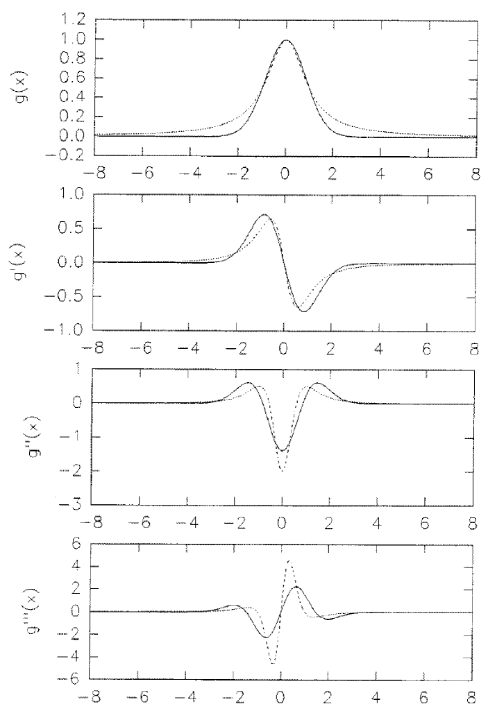
Figure 3.2: NMR line shape and derivatives for Lorentzian and Gaussian lines. The solid lines are from the Gaussian $g_{g}(x)$ and the broken lines are from the Lorentzian $g_{l}(x)$. The upper graph shows the functions $g_{g}(x)$ and $g_{l}(x)$; below are the first, second and third derivatives with respect to $x$, denoted $g^{\prime}$, $g^{\prime\prime}$ and $g^{\prime\prime\prime}$ respectively.

Modulation of either the frequency or field may, with suitable scaling, be represented as a modulation of the parameter $x$. In the limiting case of small modulation ($\Delta x_{m}\ll 1$), the $n^{th}$ harmonic response will give the $n^{th}$ derivative. In this work we refer to the fundamental as the $1^{st}$ harmonic, twice the fundamental frequency as the $2^{nd}$ harmonic and so on. Note however, that the amplitude of the $n^{th}$ harmonic signal is proportional to $(\Delta x_{m})^{n}$, where $\Delta x_{m}$ is the modulation width.

3.3.2 Sample cells

The most common CW configuration for radio-frequency operation is the ‘marginal oscillator’ which uses a resonant circuit containing the sample to form part of the oscillator. This is typically achieved by putting the sample inside the inductor of an $LC$ tuned circuit. Resonant absorption causes a small reduction in the quality factor of the circuit, resulting in a change in the output amplitude. Modulation of the RF or of the applied field is used to overcome noise and drift.

At microwave frequencies it is not possible to use lumped circuits; instead distributed elements are used (waveguides, coaxial resonators etc.). Figure 3.3 shows two possible experimental configurations. Coaxial resonators operating as reflection cells were used to obtain all the data reported in this work. As shown in figure 3.3, a circulator is used to direct the incident microwave power to the reflection cell and the reflected power to the detector. Cavity resonators operating as transmission cells with separate drive and detection ports have been used for CW NMR by Bleaney et al [11]. Cavity resonators and a circulator are also used in the Manchester pulsed spectrometer [21], albeit with resonator $Q$ limited by the maximum acceptable ring-time. A significant advantage of reflection cells is they have only one coupling to a transmission line which makes adjustment of the coupling easier than for transmission cells where there are two couplings.

 

 

Figure 3.3: Two possible CW NMR configurations: a) reflection cell and b) transmission cell. In both configurations the cell may be either resonant or non-resonant.

A non-resonant transmission cell may be useful when large amounts of material are available. The best approach is to pack a section of transmission line or waveguide with sample, partially replacing the dielectric. NMR is detected by the decrease in transmitted power at resonance. Cowan and Cha [26] have studied terbium metal using a transmission cell with a temperature sweep at fixed frequency. Ferromagnetic HoFe₂ has been studied by Ross [67] as a powder in a transmission cell using frequency sweep.

Cowan and Cha [26] used finely ground Tb powder to maximise the effective sample volume which is otherwise limited by the skin depth. They managed to measure the hyperfine splittings at temperatures up to 160 K, exceptionally high for rare-earth NMR. The line widths observed ranged from 10–50 MHz which gave well resolved quadrupole structure; the quadrupole splitting of ferromagnetic Tb at 4.2 K is $>600$ MHz with the central line at $\approx 3.1$ GHz. Initially, they used frequency sweeps but found problems with power and backgound fluctuations. They found that the background was reduced by over an order of magnitude by sweeping the temperature whilst keeping the frequency constant. Sweeping the temperature effectively sweeps the field at the nuclei because the thermally averaged electronic moment changes. In Tb the lifetime of the electronic states at temperatures above 80 K is short compared to the period of the nuclear precession. This means that the nucleus experiences an effective hyperfine field proportional to the thermal average of the electronic moment, which decreases with increasing temperature. In the present work, which is concerned with insulating rare-earth compounds at liquid helium temperatures, the lifetime of the electronic states is long compared to the period of nuclear precession and the effective hyperfine field is determined by the electronic ground state (see Bunbury et al [18]).

A major disadvantage of non-resonant over resonant cells is that of reduced sensitivity. To achieve equal sensitivity, a completely filled non-resonant cell with length of order $qQ\lambda$ is required to compete with a resonant cell of quality factor $Q$ and filling factor $q$ ($\lambda$ is the wavelength of the microwaves in the cell). The required sample volume is often unacceptably large. Powdered samples often used and generally the particles are randomly oriented. Thus, any externally applied field is randomly oriented with respect to the crystal axes of the individual particles. In general, this will result in different NMR spectra from the individual particles and hence in gross macroscopic inhomogeneous broadening. Thus, powder samples are usually used only for spontaneously magnetized materials. Non-resonant cells are clearly unsuitable for small single crystal samples. In that case a resonator with small effective cell volume and high $Q$ provides the greatest sensitivity.

Whilst offering high sensitivity, resonant cells have associated technical difficulties, especially when the $Q$ is high. First, the microwave frequency must be kept close to the resonator frequency. This may require some form of servo system either for the resonator tuning or the microwave frequency. Also, if frequency modulation is used the response of the resonator may dominate the received signal. However, these problems are surmountable: see section 3.3.8.

3.3.3 Detection systems

Microwave diode detectors produce an output voltage approximately proportional to the input power for low input power. As the input power increases they gradually change from ‘square law’ to ‘linear law’ with the output power proportional to the input power, ie. with an output voltage proportional to the square root of the input power (assuming a constant load impedance). Diode detectors are reliable and easy to use. A more sensitive method of detection is to use a low-temperature bolometer. Si and InSb bolometers are commercially available with high sensitivity at helium temperatures. However, their response is slow and would limit the modulation rate to about 500 Hz.

It is also possible to detect NMR by the temperature rise of the sample caused by resonant absorption. The temperature can be measured by mounting the sample on a thermistor. At helium temperatures the temperature coefficient can be very high so it is possible to detect very small temperature changes. Sensitivity to NMR obviously depends on the strength of resonance and on the spin-lattice relaxation time $T_{1}$.

Whatever the detector, it is desirable to use a lock-in amplifier referenced to the modulation frequency or some harmonic. Clearly, if the response time of the detection system is long then the modulation frequency must be limited. In this work we have used a diode detector, and detector noise was not the sensitivity limiting factor.

3.3.4 Quarter-wave coaxial resonator

All the NMR data in this thesis were taken using tunable truncated quarter-wave coaxial resonators. First, consider the simplified section through a (non-truncated) quarter-wave coaxial resonator shown in figure 3.4.

 

 

Figure 3.4: Simplified section through a quarter-wave coaxial resonator.

Ignoring end effects we may write down the current in the central conductor as a function of position $z$ for the lowest frequency mode ($l=\lambda/4$):

$$I(z)=I_{0}\cos\left(\frac{2\pi z}{\lambda}\right)$$ (3.19)

and hence the magnetic field distribution:

$$B(r,z)=\frac{\mu}{2\pi r}I_{0}\cos\left(\frac{2\pi z}{\lambda}\right)$$ (3.20)

We immediately see that the best position for a small sample is on the surface of the central conductor at the closed end of the resonator. In the previous work of McMorrow [51] and of Carboni et al [21], metallic single crystals have been used as the central conductor. With a metallic sample the active sample volume is severely limited by the skin effect. At GHz frequencies the skin depth is typically 1 $\mu$m at low temperatures. Using the sample as the central conductor places the active part at the ideal position in the cavity.

To make a resonator for frequency $\omega_{0}$ the central conductor length is given by

$$l\approx\frac{\pi c}{2\omega}$$ (3.21)

where $c$ is the microwave propagation speed in the resonator. To a good approximation, if the resonator is full of liquid helium then $\mu\approx\mu_{0}$ and $\epsilon\sim\epsilon_{0}$ so $c\approx c_{0}=1/\sqrt{\mu_{0}\epsilon_{0}}$. For resonance at 5 GHz, equation 3.21 gives a central conductor length of $\approx 15$ mm. Note, however, that sample resonance can cause a significant change in the effective $\mu$ averaged over the resonator volume which changes the resonant frequency.

The resonator can be made tunable by adding a piston at the ‘open’ end which provides a capacitance at the end of the central conductor. We now call it a truncated quarter-wave coaxial resonator. If the separation $d$ between the end of the central conductor and the piston is small compared to the radius of the end of the central conductor then, ignoring end effects,

$$d=\epsilon AZ_{0}\omega_{0}\tan\left(\frac{\omega_{0}l}{c}\right),$$ (3.22)

where $A$ is the end area of the central conductor; and

$$Z_{0}=\frac{1}{2\pi}\sqrt{\frac{\mu}{\epsilon}}\ln\left(\frac{b}{a}\right).$$ (3.23)

The expression for $d$ is due to Carboni [19], who plots theoretical curves against measured values showing reasonable agreement.

It is convenient to use the concept of the ‘line width’ of the resonator which we simply define as

$$\Delta\omega_{r}=\frac{\omega_{0}}{Q},$$ (3.24)

where $\omega_{0}$ is the resonant frequency and $Q$ is the quality factor. The $Q$ and hence the line width $\Delta\omega_{r}$ depend on the coupling to the resonator and on any resonant absorption inside the resonator. We use the term intrinsic $Q$ to refer to the $Q$ of the resonator in isolation; and loaded $Q$ to refer to the $Q$ of the resonator coupled to a transmission line. Both of these quantities are defined in the absence of NMR and we subsequently consider any resonant absorption as a perturbation.

3.3.5 Parallel-$LC\!R$ resonator model

To model NMR in a resonator, it is convenient to consider an electrical analogue of the microwave resonator. Figure 3.5 shows a parallel-$LC\!R$ circuit where the sample NMR can be modelled by a change in the value of $L$: see section 3.3.7.

 

 

Figure 3.5: Parellel-$LC\!R$ analogue of a resonator.

The resonator must be coupled to the microwave source and to the detector. This can be achieved with one or two transmission lines terminated with ‘loops’ protruding into the resonator so that the current is coupled to the RF magnetic field in the resonator. In this work we have used a reflection cell so we consider the case of a single coupling loop. The coupling of the transmission line to the resonator provides an impedance conversion. This is accounted for by transforming the impedance of the resonator analogue such that we can consider it as if it were directly connected to the transmission line.

To define the resonator parameters, consider the system in the absence of NMR. Any non-resonant losses in the sample are included in the quality factor $Q$ and are effectively lumped into $R$. The inductance, $L=L_{0}$ ‘off-NMR’ and the resonant frequency is simply

$$\omega_{0}=\frac{1}{\sqrt{L_{0}C}}.$$ (3.25)

3.3.6 Coupling to a resonator

We first consider just the resonator when the sample is well off NMR resonance. If the resonance frequency of the resonator is $\omega_{0}$; the intrinsic $Q$ is $Q_{0}$; and the inductance in the equivalent parallel-$LC\!R$ circuit is $L_{0}$ then, on resonance, the admittance is

$$Y_{0}=Y(\omega_{0})=\frac{1}{\omega_{0}Q_{0}L_{0}}.$$ (3.26)

If the characterisctic admittance of the transmission line is $Y_{t}$, we define the coupling coefficient $\alpha$ as,

$$\alpha=\frac{Y_{t}}{Y_{0}}.$$ (3.27)

The regime $\alpha<1$ is referred to as under-coupling; $\alpha=1$ as critical coupling; and $\alpha>1$ as overcoupling. If two transmission lines are used the transfer characteristic will be more complex than the case of a single transmission line, involving both couplings. Here we restrict discussion to single port resonators as used for this work. From equation 3.27 the voltage reflection coefficient $\rho(\omega)$ follows as

$$\rho(\omega)=\frac{\alpha Y_{0}-Y(\omega)}{\alpha Y_{0}+Y(\omega)}.$$ (3.28)

 

 

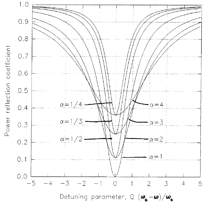
Figure 3.6: Power reflection coefficients $\mid\rho^{2}(\omega)\mid$ for different degrees of coupling as a function of the detuning.

Figure 3.6 shows the power reflection coefficient $\mid\rho^{2}(\omega)\mid$ as a function of the detuning. The loaded resonator line width is increased by over-coupling but is decreased by under-coupling, relative to critical coupling. The $Q$ of a critically coupled resonator is half that of the same resonator unloaded (ie. in the limit infinite under-coupling $\alpha\rightarrow 0$, when $Q\rightarrow Q_{0}$).

In practice the coupling depends critically on both the position and orientation of the coupling loop. Adjustment is achieved by sliding and twisting the transmission line with the coupling loop at the end. However, it is hard to know what the coupling is except in the region of critical coupling where the reflected power falls to zero on resonance. It is often not even easy to see whether the system is slightly under- or over-coupled.

3.3.7 NMR in a resonator

This section discusses the effect of NMR on the response of a resonant reflection cell. The transverse RF nuclear susceptibility of the sample $\chi_{s}$, can be represented by a change in $L$:

$$L=L_{0}(1+q\chi_{s}),$$ (3.29)

where $q$ is the filling factor and $\chi_{s}=\chi^{\prime}_{s}-i\chi^{\prime\prime}_{s}$. Expanding the inductance to an explicitly complex form gives

$$L=L_{0}(1+q\chi^{\prime}_{s}-iq\chi^{\prime\prime}_{s}).$$ (3.30)

The imaginary part of the susceptibility $\chi^{\prime\prime}_{s}$ is chosen with the negative sign so that positive $\chi^{\prime\prime}_{s}$ represents absorption. This can be seen by considering the impedance of $L$:

$$Z_{L}=\omega L_{0}q\chi^{\prime\prime}_{s}+i\omega L_{0}(1+q\chi^{\prime}_{s}),$$ (3.31)

where positive $\chi^{\prime\prime}_{s}$ gives a positive resistance. It is convenient to transform this series impedance into a parallel admittance. Assuming ${\mid q\chi_{s}\mid}\ll 1$ and working to first order in $\chi^{\prime}_{s}$ and $\chi^{\prime\prime}_{s}$ gives

$$Y_{L}\approx\frac{q\chi^{\prime\prime}_{s}}{\omega L_{0}}-\frac{i(1-q\chi^{\prime}_{s})}{\omega L_{0}}.$$ (3.32)

This is equivalent to a resistance $(\omega L_{0})/(q\chi^{\prime\prime}_{s})$ in parallel with an inductance $L_{0}(1+q\chi^{\prime}_{s})$. Having performed this transformation the admittance of the resonator follows simply, and dividing by $Y_{0}$ gives

$$\frac{Y(\omega)}{Y_{0}}\approx\left\{1+\frac{Q_{0}\omega_{0}q\chi^{\prime\prime}_{s}}{\omega}\right\}+iQ_{0}\left\{\frac{\omega^{2}-\omega_{0}^{2}(1-q\chi^{\prime}_{s})}{\omega\omega_{0}}\right\}.$$ (3.33)

To find the transfer charactersic of the system we must consider this admittance connected to the transmission line. The voltage reflection coefficient is given by equation 3.28 and $\mid\rho^{2}(\omega)\mid$ is the power reflection coefficient. In an experiment using a resonator and square law detector, the output voltage is proportion to $\mid\rho^{2}(\omega)\mid$ provided the input power remains constant.

 

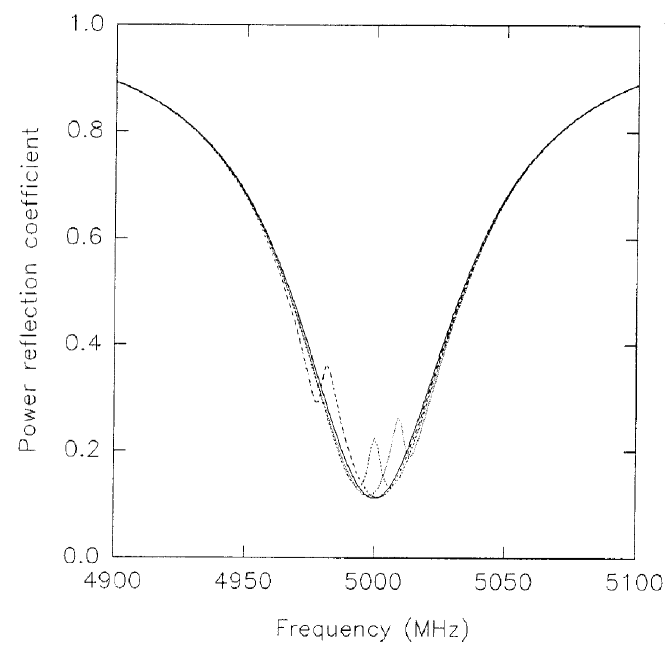
solid line	no NMR
long dash	$\omega_{s}/2\pi$=4980 MHz
medium dash	$\omega_{s}/2\pi$=5000 MHz
short dash	$\omega_{s}/2\pi$=5010 MHz

 

Figure 3.7: Power reflection coefficients as a function of frequency for a cavity with intrinsic $Q_{r}=100$ and a sample $Q_{s}=1000$ with the cavity under-coupled ($\alpha=0.5$).

 

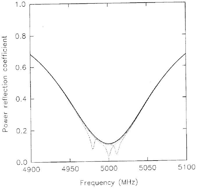
solid line	no NMR
long dash	$\omega_{s}/2\pi$=4980 MHz
medium dash	$\omega_{s}/2\pi$=5000 MHz
short dash	$\omega_{s}/2\pi$=5010 MHz

 

Figure 3.8: Power reflection coefficients as a function of frequency for a resonator with intrinsic $Q_{r}=100$ and a sample $Q_{s}=1000$ with the cavity over-coupled ($\alpha=2$).

Figures 3.7 and 3.8 show the effect of a NMR resonance that is narrow relative to the resonator line width. The intrinsic $Q$ of the resonator $Q_{r}$ is taken as 100 which gives a loaded $Q\approx 50$ around critical coupling. The sample line width $\Delta\omega_{s}=\omega/Q_{s}$ where it is convenient to consider the sample ‘quality factor’ $Q_{s}$ for comparison with that of the resonator. We have taken $Q_{s}=1000=10Q_{r}$ have chosen the resonance frequency of the resonator as $\omega_{0}/2\pi=5000$ MHz so that the frequencies are of the correct order for rare-earth NMR. The strength of the NMR is deliberately exaggerated.

The optimal value of the coupling coefficient $\alpha$ depends on the type of detector. If the detector is ‘linear’ then the NMR signal is maximised for critical coupling ($\alpha=1$); if it is ‘square-law’ then $\alpha=2\pm\sqrt{3}$ is optimal. In practice we have used coupling fairly close to critical, approximately $0.5<\alpha<2$. Here we take $\alpha=0.5$ and $\alpha=2$ as examples. Figure 3.7 is for an under-coupled resonator, and figure 3.8 is for an over-coupled resonator. In both cases the solid line is the resonator resonance curve without NMR ($\omega_{0}/2\pi=5000$); three other curves are shown for NMR resonances at $\omega_{s}/2\pi=4980$, $5000$ and $5010$ MHz. Although the curves for over- and under-coupling are significantly different, they both show that the NMR resonance creates a sharp and, unless $\omega_{s}=\omega_{0}$, asymmetric change in the reflection coefficient. Consider a frequency modulation experiment where the carrier frequency is somehow kept tuned to the resonator resonance. It is clear that varying amounts of harmonics will be generated from a sinusoidal frequency modulation as the sample resonance frequency moves relative to the resonator frequency: see section 3.3.8. Although this case usefully illustrates the harmonic generation, in practice we have used resonators with $Q_{r}$ higher than $Q_{s}$ for the systems studied.

 

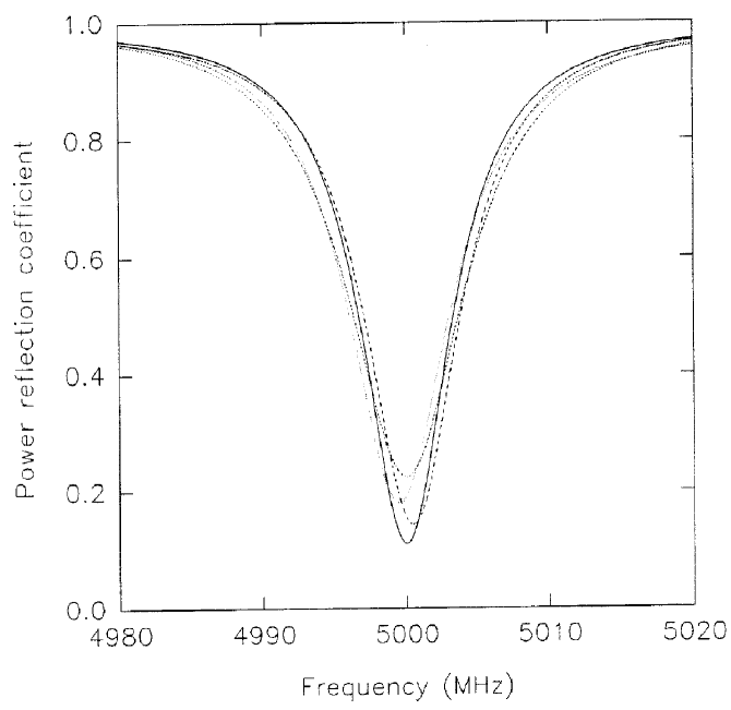
solid line	no NMR
long dash	$\omega_{s}/2\pi$=4980 MHz
medium dash	$\omega_{s}/2\pi$=5000 MHz
short dash	$\omega_{s}/2\pi$=5010 MHz

 

Figure 3.9: Power reflection coefficients as a function of frequency for a resonator with intrinsic $Q_{r}=1000$ and a sample $Q_{s}=100$ with the cavity under-coupled ($\alpha=0.5$).

 

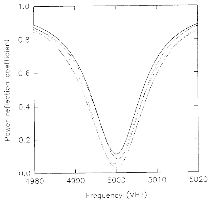
solid line	no NMR
long dash	$\omega_{s}/2\pi$=4980 MHz
medium dash	$\omega_{s}/2\pi$=5000 MHz
short dash	$\omega_{s}/2\pi$=5010 MHz

 

Figure 3.10: Power reflection coefficients as a function of frequency for a resonator with intrinsic $Q_{r}=1000$ and a sample $Q_{s}=100$ with the cavity over-coupled ($\alpha=2$).

Figures 3.9 and 3.10 show the more realistic situation of $Q_{r}=1000$ and $Q_{s}=100$. Except for the swapping the line widths of the resonator and NMR, the other parameters are as for figures 3.7 and 3.8. With the NMR resonance much broader than the resonator resonance we cannot expect sharp variations in the reflection coefficient to be caused by NMR. However, there are definite changes in the magnitude of the reflection coefficient and in the resonance frequency (discussed below). As before, the power reflection coefficient is increased for under-coupling but decreased for over-coupling. There is also a small asymmetry that will generate odd harmonics from a sinusoidal frequency modulation about the centre of the combined resonance: see section 3.3.8.

From figures 3.9 and 3.10 there is clearly a shift in the cavity resonance frequency when the sample resonance is close to it. This results primarily from the dispersive part of the sample susceptibility. The the cavity resonance occurs when the admittances of the inductance and the capacitance cancel.

To first order in $\chi^{\prime}_{s}$ the cavity resonance frequency is:

$$\omega_{r}\approx\frac{1}{\sqrt{L_{0}(1+q\chi^{\prime}_{s})C}}\approx\omega_{0}\left(1-\frac{q\chi^{\prime}_{s}}{2}\right).$$ (3.34)

This expression is useful only when the sample line width is greater than the resonator line width so that $\chi^{\prime}_{s}$ is approximately constant over the centre portion of the resonator resonance.

Recalling equation 3.10, around the sample resonance we expect the resonator frequency to be increased when the $\omega_{s}>\omega_{0}$; equal the natural resonant frequency when $\omega_{r}=\omega_{s}=\omega_{0}$; and be reduced when $\omega_{s}<\omega_{0}$. These inequalities are not affected by the strength of the coupling. We have used this method to detect NMR, see section 4.7.3.

3.3.8 Frequency modulation with a resonator

The use of frequency modulation with a resonator is unusual but has given good results (see chapter 5). If the NMR line width is small compared to the resonator line width it is easy to see how harmonics of the sinusoidal frequency modulation are generated by the NMR resonance. If the modulation amplitude is comparable to the NMR line width it will differentiate the ‘sharp’ NMR line from the broader resonator resonance. Although this situation could be engineered by designing a low $Q$ resonator, the low $Q$ will reduce the sensitivity of the spectrometer. In our experiments we have opted for a high $Q$ resonator so that the resonator line width is much less than the NMR line width. In that case it is not practical to use a modulation amplitude comparable to the NMR line width.

If we keep the carrier frequency at the ‘centre’ of the combined resonator and sample resonance, in the absence of NMR the symmetric resonator line will generate only even harmonics of the modulation and the fundemental will be supressed. The harmonic response of the resonator is essentially like the derivatives of a Lorentzian NMR absorption (see figure 3.2). As the NMR resonance is swept though the resonator resonance, or conversely, the overall line shape will be asymmetric and even and odd harmonics will be generated. However, because the response of the system is dominated by the roughly symmetric resonator resonance which generates mainly even harmonics, we choose to detect NMR using an odd harmonic of the modulation frequency.

In practice, it is necessary to use feedback to keep the microwave frequency accurately to the combined resonator and sample resonance. In the absence of NMR, all odd harmonics of the resonator response are zero at the resonant frequency if we assume a symmetric resonator resonance. Thus, using the first harmonic as an error signal, the carrier frequency of the microwave oscillator can be locked to the combined resonance. NMR will cause a shift in the frequency at which the first harmonic signal is zero (see figures 3.9 and 3.10) and thus in the locked carrier frequency. Obviously, this means that the first harmonic cannot be used to detect NMR. However, the NMR also creates an asymmetry in the combined resonator and sample response which generates higher harmonics that can be used to detect NMR. In the regime $Q_{r}\gg Q_{s}$ it is not practicable to use a modulation deviation that is comparable to the NMR line width. The resonator line width puts a limit on the maximum practical modulation deviation. Thus $\Delta\omega_{m}\ll\Delta\omega_{s}$, which imposes a significant sensitivity penalty on the use of higher harmonics: approximately,

$$\mbox{sensitivity}\propto\left(\frac{\Delta\omega_{m}}{\Delta\omega_{s}}\right)^{n}$$ (3.35)

where $\Delta\omega_{m}$ is the frequency modulation amplitude, $\Delta\omega_{s}$ is the NMR line width, and $n$ is the detection harmonic. Thus third harmonic detection is the best option when $Q_{r}\gg Q_{s}$.

Ideally the third harmonic signal will be zero when off the NMR resonance. However, this is not the case in practice because of imperfect locking to the resonator and asymmetries in the overall transmission function of the microwave system. Fluctuations in the ‘background’ third harmonic signal are a significant contribution to the total noise.

Chapter 4 The CW microwave NMR spectrometer

Some of the requirements of a CW spectrometer for NMR spectroscopy of rare-earth ions in solids have been discussed in chapter 3. In particular, the relative merits of ‘sweep’ and modulation in the field and frequency domains have been considered. The spectrometer has been built to allow any combination of sweep and modulation. Also, there are facilities to lock the carrier frequency to the combined resonator and sample resonance, and to allow harmonic detection.

This chapter describes the spectrometer as built. Although we concentrate on field sweep experiments, the spectometer has been designed with flexibility in mind. The spectrometer architecture and arrangements for field and frequency modulation experiments is described in section 4.1. The microwave system and circuits used to set up the spectrometer are described in section 4.2. Computer control has been implemented from the start and has influenced the organisation of the system. In particular, parts of the system controlled by the computer are grouped in the ‘interface unit’ (section 4.3).

The current operating frequency range of the spectrometer is 4–8 GHz. However, it would be straightforward to extend the frequency range to 2–8 GHz: simple modifications to the microwave system and to the software would be required. These are described in the appropriate sections.

The spectrometer has been used successfully only with field sweeps (section 4.7.1). Frequency sweeps have been attempted on several occasions but the background has proved very much larger than any expected signal. Section 4.7.2 discusses the frequency sweep method a little further but otherwise we consider only the field sweep method. Also, and as a counter-example to the accepted wisdom that modulation is required, section 4.7.3 reports detection of NMR by the shift in the resonator frequency and by the change in reflected power, both without modulation.

4.1 Spectrometer architecture

First, consider the experimental apparatus. Figure 4.1 shows the main parts of the apparatus and the principal interconnections. The computer is an IBM PC compatible with two interface cards: an IEEE488 bus interface (Brain Boxes Ltd., ‘Elite’ card) and a parallel input/output (PIO) card. The PIO card is used to drive the instrument interface via a buffering and signal conditioning card. The interface, the instrument unit and the cards it contains are described in section 4.3. The microwave system, ‘tuning circuit’ and ‘frequency locking circuit’ are described in section 4.2.

 

 

Figure 4.1: Block diagram of the CW NMR spectrometer hardware (shown arranged for a frequency modulation experiment).

The tuning circuit provides the facility to sweep the transmitter frequency about a nominal centre frequency set by the computer. The sweep waveform and reflected power signal (detector DC output) are used to provide an oscilloscope display of reflected power against frequency. Typically, the display shows a dip in the reflected power corresponding to the resonator resonance. The resonator can be critically coupled by adjusting the coupling until the reflected power goes to zero on resonance. In the actual NMR experiment the tuning circuit has no function except to connect the reflected power signal to the lock-in amplifier.

In all experimental configurations (frequency modulation, field modulation and ‘no’ modulation) we have used some frequency modulation. Where this is not used to detect NMR, only a small deviation (typically 0.5 MHz) is used. The frequency locking circuit is used to select ‘tuning’ mode or ‘normal’ mode. In normal mode the transmitter frequency is locked to the resonator frequency by nulling the first harmonic signal generated by the frequency modulation. This is done by using the output of the first harmonic lock-in (fsig) as an error signal which controls the microwave frequency via the oscillator control card (YIG-tuned oscillator control card, section 4.3.1). In tuning mode the frequency locking circuit simply connects the sweep signal from the tuning circuit to the sweep input of the oscillator control card.

In the following two sections we outline the frequency and field modulation techniques used for this work. The arrangement ‘without’ modulation is essentially a simplification of the arrangement for either of these techniques: just the frequency locking circuit and DC detection.

4.1.1 Frequency modulation technique

Frequency modulation is easy to implement and has previously been used for CW NMR at Manchester by Ross [67]. However, the earlier experiments used transmission cells with reasonably flat frequency response. In this work we adopted the unusual combination of frequency modulation and a resonant cell. This gives the benefit of $Q$ but problems with background from the resonator response (section 3.3.2). In particular, the experiment must be performed close to the resonant frequency of the resonator. This requirement becomes more stringent with increasing resonator $Q$.

For maximum response the frequency deviation of the modulation should be comparable to line width of the NMR. However, there is no point in using a frequency deviation larger than the resonator line width because there will be little excitation when off resonance. This gives the rough condition that the modulation deviation should not be larger than either the resonator or NMR line widths.

Figure 4.2 shows the two ‘circuits’ that are fundamental to this configuration. Firstly, the frequency locking loop uses a lock-in amplifier at the modulation frequency to tune the microwave transmitter so that the first harmonic signal is zero. Assuming that the resonator line shape is symmetric, at least over the width of the modulation, this will lock the source to the centre of the resonance. This is very important with high $Q$ resonators, particularly if the field sweep causes a shift in the resonator frequency. With a paramagnetic sample the dominant shift is due to the fall in differential susceptibility as the magnetization is saturated. Shifts of up to 20 MHz have been seen in HoF₃ (0–8 T). We have also found that the feedback loop can improve the frequency stability of the transmitter; see section 4.5.2. For the frequency locking loop to work properly, the frequency excursion should be smaller than the resonator line width; however we have already argued that this is compatible with efficient NMR excitation so no additional constraints are imposed.

Secondly, there is the measurement circuit. The reference at $n$ times the modulation frequency is used to detect the $n^{th}$ harmonic with a 2-phase lock-in amplifier. It is not strictly necessary to have a 2-phase lock-in amplifier, but the phase of the harmonic signal was found to vary significantly with time and the microwave frequency, and taking just the magnitude (rms of the 2-phases) gave the best results. This lock-in amplifier is equipped with an IEEE488 interface and readings are recorded by the computer.

In operation, the spectrometer is set up with the transmitter frequency locked to the resonator resonance by the frequency locking circuit, and the applied field is swept through some range. As the field changes, the computer records the field, frequency, harmonic output and any other parameters requested (that can be monitored either directly; with an additional IEEE488 equipped DMM; or using one of the spare analogue-to-digital converter inputs). The software is described in section 4.4. Not shown in the schematic is the levelling loop with which the microwave power output of the source is kept constant.

 

 

Figure 4.2: Schematic of the experimental configuration for a frequency modulation CW NMR experiment.

4.1.2 Field modulation technique

Field modulation may be produced using either the main solenoid or an additional field coil. In practice, it is not possible to modulate the main solenoid current at more than a few hertz because of its high inductance, $\approx$10 H. Modulation of 1 mT at 10 Hz would produce $\approx$6.6 V back-emf and the magnet power supply cuts out if the voltage across the magnet terminals exceeds 5 V. Using the main solenoid would also mean that all the metalwork of the resonator, support system and solenoid former would be within the modulation field and subject to eddy-current heating. An additional field coil has therefore been wound directly onto the resonator, with a much smaller area enclosed and hence a much smaller inductance. The field coil is described in section 4.5.1. It has an inductance of $\approx$0.12 mH and the back-emf is not a significant problem. The factor limiting the modulation field and frequency is eddy-current heating of the resonator. Typically, modulations of 1–10 mT at $\approx$100 Hz were attainable without unacceptable heating.

Figure 4.3 shows the experimental configuration schematically. The microwave transmitter and resonator frequencies are not stable enough over time or with field for the transmitter to stay tuned to the resonance without feedback. The frequency locking loop described in the preceeding section was therefore used, but with a frequency excursion small (typically $\pm$0.5 MHz) compared to the resonator and NMR line widths. The frequency of this modulation was typically 100 kHz and no problems of interference with the low frequency field modulation were encountered.

The field modulation coil is driven by a power amplifier designed to provide up to $\pm 3$ A into a low-impedance inductive load. The modulation signal and square-wave reference are generated by an audio frequency oscillator (Thandar type TG102) and the response measured using the 2-phase lock-in amplifier. The in-phase signal gave good derivative spectra indicating little phase shift in the system at the operating frequency. As in the frequency modulation experiments, the applied field was swept through some range with the computer storing the readings.

 

 

Figure 4.3: Schematic of the experimental configuration for a field modulation CW NMR experiment.

4.2 Microwave system

The microwave system is very simple: it consists of a transmitter, circulator, resonator containing the sample and a detector (figure 4.4). The quarter-wave coaxial resonators are described, in section 4.5. Semi-rigid coaxial cable (0.141" diameter with PTFE dielectric and SMA connectors) is used for microwave connections in the source and from the cryostat top-plate down to the resonator. The other microwave connections use flexible coaxial cables (Suhner Ltd., ‘Sucoflex’).

 

 

Figure 4.4: CW NMR configuration using a circulator and resonator.

This section also includes descriptions of the ‘tuning circuit’ and the ‘frequency locking circuit’ which are not part of the microwave system per se. They are, however, very important in tuning the system.

4.2.1 Microwave transmitter

Figure 4.5 shows schematically the arrangement of microwave components comprising the transmitter. The oscillator output is divided between two arms by a 3 dB splitter. Half of the power is used to provide an output for frequency measurement. The additional -10 dB directional coupler in this arm was used to provide an output for a prescaler that has not been implemented. The other arm uses an electronic attenuator (Hewlet Packard type 33142A) and an amplifier (described below) to provide variable output power from $<$0.1 mW to $\approx$130 mW. The directional detector (Krytar type 1211S, 1–12.4 GHz) allows the output power to be monitored. Usually the output power is levelled, keeping the directional detector output (level out) constant by feedback to the level control input. However, the levelling loop control card (section 4.3.2) provides the facility of levelling the power at another detector. For example, it might be best to level the transmitted power in an experiment using a non-resonant transmission cell.

 

 

Figure 4.5: Schematic of the microwave transmitter.

The oscillator (Philips/Sivers Lab. type PM 7020C) is based on a transistor coupled to an yttrium-iron-garnet (YIG) resonator. The YIG resonator has high $Q$ and is tuned by changing the applied field. The oscillator is tunable over the range 4–8 GHz with power output varying between 22 and 39 mW over that range (measured). Other devices are available to cover the range 2–8 GHz. In addition to the tuning coil, the oscillator has another small coil to allow frequency modulation (FM). This provides up to $\pm$50 MHz deviation with a bandwidth from DC to 100 kHz (-3 dB).

The noise output of YIG-tuned oscillators is low, typically 50 dB down on the fundemental; however there is a much larger harmonic content. The oscillator used is specified to have total harmonic content more than 12 dB down on the fundemental. The current system operates over just one octave (4–8 GHz) and harmonics will be outside the bandwidth of the amplifier and considerably attenuated. Microwave noise has not been a significant problem. However, harmonics could be more of a problem in a 2–8 GHz system where, between 2 and 2.7 GHz, both second and third harmonics would be within the system bandwidth.

The amplifier (Avantek Inc. type AWT-8052) is a 2–8 GHz device providing $\approx$17 dB gain with a maximum output power of $\approx$130 mW (21 dBm). Modifying the source to cover 2–8 GHz would simply require replacement of the oscillator.

4.2.2 Circulator

Circulators are available covering octave bands and the spectrometer uses a 4–8 GHz device. Extension of the spectrometer operating range to cover 2–8 GHz would require two circulators which could either be manually exchanged or switched in and out using microwave relays. Ideally, circulators should not be placed in magnetic fields but no problems have been experienced with the circulator only 1.5 m from the 8 T magnet (roughly on axis).

4.2.3 Detector

The microwave detector uses a GaAs ‘planar-doped barrier’ diode matched to the 50 $\Omega$ transmission line by a miniature thin film circuit. Details are given below:

Hewlet Packard, type HP33334C.
Frequency range 0.01–33 GHz, response flat to $\pm$0.45 dB over 0.01–26.5 GHz.
Maximum continuous input power 200 mW (23 dBm).

The detector and a pre-amplifier are built into a shielded box (figure 4.6). Separately buffered AC and DC coupled outputs are provided. The DC coupled output is used for tuning and to monitor operation of the frequency locking circuit. The AC coupled output is connected to the 2-phase lock-in amplifier.

 

 

Figure 4.6: Schematic of the microwave detector and pre-amplifier.

4.2.4 Tuning circuit

This circuit is required to set up the spectrometer prior to NMR measurement, and is shown schematically in figure 4.7. The computer sets the nominal microwave frequency and in ‘tune’ mode the tuning circuit provides a symmetric frequency sweep about this frequency. A calibrated dial allows the sweep range to be adjusted between 0 and 1 GHz ($\pm$500 MHz). The YIG sweep output controls the microwave frequency via external sweep input of the oscillator control card. A second output provides a $\pm$1 V triangular voltage waveform to control the oscilloscope X-deflection. The detector DC output (reflected microwave power) is buffered to provide the Y-deflection, and there is a straight-through connection to the first harmonic lock-in.

The usual method of operation is initially to set the sweep to a wide frequency range to find the resonator resonance. When the resonance is located, the coupling can be adjusted roughly for low reflected power on resonance. Then the resonator can be tuned to the desired frequency and the sweep range gradually turned down for greater resolution. This facility is useful for checking the resonator $Q$ and for fine adjustment of the coupling. Once the source is centred on the resonance the frequency locking circuit can be switched in. Without adjusting the oscilloscope, the state of the frequency locking loop is shown by the reflected power trace; see the following section. The X-deflection provides a convenient timebase without having to adjust the oscilloscope.

 

 

Figure 4.7: Schematic of the tuning circuit.

4.2.5 Frequency locking circuit

This circuit uses the first harmonic signal from the lock-in amplifier as an error signal which is amplified, filtered and fed back to control the microwave frequency. Figure 4.8 shows the circuit schematically. The principle of operation is that the first harmonic in-phase signal will approximate to the derivative of the resonator line shape. This will be zero at the centre of the resonance, so using feedback to adjust the microwave frequency until the first harmonic signal is zero will lock the system to the resonator frequency.

When the microwave frequency is within the resonator line width the frequency locking circuit can be switched in (normal). We have found it best to start with the loop gain turned right down ($\approx$0) and then slowly increase the gain (slowly with respect to the time constant of the lock-in). Usually the loop will lock at some point, indicated by the lock indicator and by a steady trace on the oscilloscope. Further increase of the gain usually improves the stability up to a point where the microwave frequency starts to oscillate. The gain can then be turned down a little to stabilise the loop. If the frequency ‘jumps’ out of the resonance the procedure can be repeated by turning the loop gain down again.

It is not practicable to predict the gain required for stability of the loop. The loop gain is affected by the resonator line width, the microwave power, the coupling to the resonator and the gain and time constant of the lock-in amplifier. The following ‘typical’ values were taken for the gains of each part of the loop: YIG-tuned oscillator tuning sensitivity $\approx 4{\times 10^{8}}$ Hz/V, resonator/detector/lock-in frequency to voltage conversion factor $\approx 4{\times 10^{-7}}$ V/Hz (resonator $Q\approx 800$, lock-in gain adjusted to give $\pm 5$ V peak first harmonic output) and frequency locking circuit amplifier gain $\approx 200$. The component values were chosen: $R1=10$ k$\Omega$, $R2=470$ $\Omega$ and $C=1$ $\mu$F, giving the loop a unity-gain frequency of $\approx$6 kHz with the filter ‘zero’ at $\approx$300 Hz for a safe phase-margin (with 30 ms lock-in time constant).

 

 

Figure 4.8: Schematic of the frequency locking circuit.

4.3 Interface unit

We use the term ‘interface unit’ to describe the unit that contains all the computer controlled interfacing and control electronics built for the spectrometer. The individual parts of the interface unit are build as ‘cards’; grouped in one unit because this allows the computer interface and power supplies to be shared. First, we describe the shared parts of interface unit, followed by descriptions of each card that it contains.

The interface unit is connected to the control computer via the home-built instrument interface. It would be preferable to connect the interface unit to the IEEE488 bus, along with the other instruments. However, the IEEE488 bus is sufficiently complicated that an interface to it would have to be controlled by a microprocessor and hence take a considerable amount of time to design and build. Such an interface could be retro-fitted in place of the current interface.

The instrument interface is controlled from the computer via a PIO card (based on the 8255 integrated circuit). Another circuit provides signal conditioning and buffering for the inputs and outputs of the PIO card. Buffering was implemented to allow the interface to operate over a long cable (10 m at present; could be longer if required) so that computer could be physically separated from the experiment if interference was a problem. The signal conditioning uses simple $RC$ filters to slow the transitions to $\approx 1$ $\mu$s, to reduce crosstalk and radiated interference. In practice, no interference problems were experienced with the PC about 3 m from the cryostat and microwave components.

The instrument interface is a simple parallel interface. There are 8 input lines, 8 output lines and 8 control signals (3 outputs, 5 inputs; directions given with respect to the computer). The 8 output lines use are used to specify either a 6 bit address and the direction of transfer, or 7 bits of output data. Two other lines are connected to allow the software to tell if the instrument is connected and if so, if the power is switched on. The software can thus respond with sensible error messages in these circumstances.

Inside the interface unit, the instrument interface is connected to the instrument bus. Physically, this is implemented as a backplane with wire-wrapped DIN41612 indirect edge-connectors. These provide 60 pins and 4 coaxial connections for each card. Multiple pins are used for separate digital and anolgue power supply connections, 24 pins are used for the bus and 12 are unused. The addresses are decoded by individual cards; the bus connections are the same to all cards. However, the positions of the cards are fixed by point-to-point coaxial connections made on the backplane. There are also special power supply connections for the YIG-oscillator control card.

Cards are built on either prototyping boards or specially designed printed circuit boards. Figure 4.9 shows a view of the instrument box with the lid off. The instrument interface is in the back-left corner and power supplies are to the back-right. The instrument bus runs across the centre (blue wires) with the individual cards to the front.

 

 

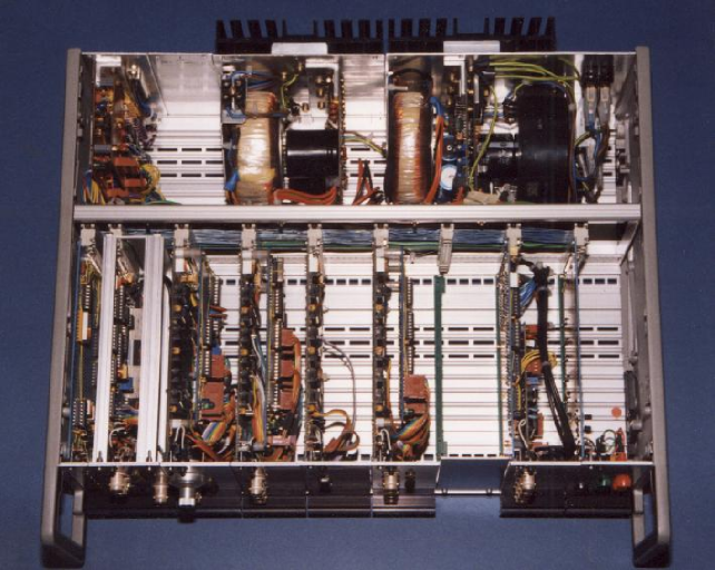
Figure 4.9: Photograph of the interface unit with lid removed showing internal organisation and contruction (the unit is $\approx$480 mm wide).

4.3.1 YIG-tuned oscillator control card

The YIG-tuned oscillator in the microwave transmitter has stringent power supply requirements which have been carefully adhered to. The power supplies have been kept separate from the supplies to the other cards. Operational amplifier based regulators are used because monolithic regulator integrated circuits are not stable enough. The regulators are located on heatsinks at the back of the intrument box with the control card providing connection to the microwave transmitter via the same cable as the tuning and modulation signals.

 

 

Figure 4.10: Schematic of the YIG-tuned oscillator control card

A 14 bit digital-to-analogue converter (DAC) provides the tuning signal for the oscillator, figure 4.10. This gives a frequency resolution of better than 300 kHz over the 4–8 GHz tuning range. The tuning linearity is limited by the oscillator and not the DAC. Linearity is not very important because the oscillator tuning can be adjusted until the measured frequency is as desired. The DAC output voltage and two sweep input voltages are summed and buffered to provide the tuning voltage. The two sweep inputs can be enabled or disabled from software using the analogue switches.

The frequency modulation coil in the oscillator gives a frequency deviation of $\pm$50 MHz for $\pm$150 mA coil drive (the maximum allowed). The coil has an inductance of $<$2 $\mu$H and a resistance of $<$1 $\Omega$. By putting 100 $\Omega$ in series with the coil the combined impedance is almost resistive over the frequency range 0–100 kHz. At 100 kHz the phase shift is $\approx$0.7^∘. This simplifies the drive amplifier and an EL2001 buffer IC was used (Elantec Ltd. available from RS Ltd.). An output swing of $\pm$10 V provides $\pm$33 MHz deviation and, with the buffer amplifier operating from $\pm$15 V power supplies, it is impossible to over-drive the modulation coil. The buffer amplifier is preceeded by a gain 10 amplifier and FM input selection switches as shown in figure 4.10. The measured performance is: $\pm$33 MHz deviation for $\pm$1 V input (saturation at $\pm$1.2 V) and frequency response from DC to $>$200 kHz (5% drop in deviation relative to DC).

The sweep inputs are used for the frequency locking loop and for tuning the resonator. The tuning circuit provides a frequency sweep adjustable up to $\pm$500 MHz. The FM inputs are used for frequency modulation, driven from either the modulation card or an external oscillator. There are internal (on the backplane) and external (on the front panel) connections for both the FM and sweep inputs.

4.3.2 Level control card

The microwave power was levelled at the output of the microwave source for the work reported in this thesis. To do this, output of the directional detector is compared with a reference voltage and the error signal is used to drive the electronic attenuator in the transmitter, completing the feedback loop. For this particular arrangement, it would be best to have the levelling loop built into the transmitter, with only the reference set by the computer. However, in the interests of flexibility, the error amplifier reference and switching circuits have been built as a card in the interface unit.

The level control card is shown schematically in figure 4.11. The input is selected from one of three connections on the front panel, or one connection on the backplane. The high-gain input (IN0) is for the directional detector in the transmitter (output 0–250 mV) and the medium-gain input (IN1) is for a detector receiving most of the oscillator output, for example the detector of a transmission cell experiment (typically 0–1 V). The other two inputs, IN2 and IN3 provide auxiliary inputs on the front panel and backplane respectively. The software selected input is compared with a reference voltage set by DAC0. The amplified error voltage is filtered by a simple low-pass filter ($\tau\approx 0.4$ s) which averages variations in amplitude caused by frequency modulation (in the range 1–100 kHz). To level the power at the modulation frequency would require a fast levelling loop with appropriate phase compensation. The arrangement described here is not suitable for that purpose. A detection circuit senses whether the error amplifier is saturated, indicating unlevelled output. The detection circuit has an LED indicator and the output can also be read by software.

The output to control the electronic attenuator in the microwave transmitter (via the driver circuit) is selected from software. Either the filtered error-amplifier output, or a DC control voltage from a second DAC (DAC1) can be selected. Direct control using DAC1 allows unlevelled operation.

 

 

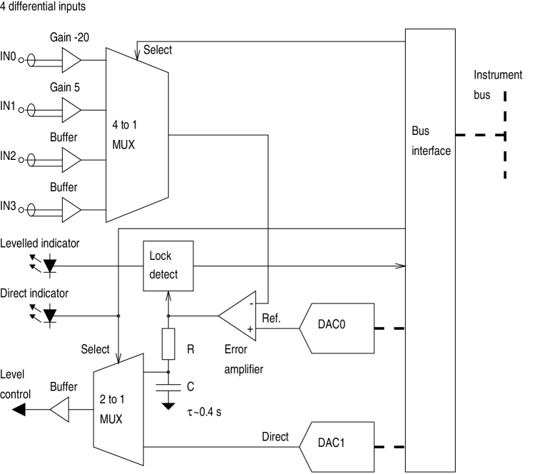
Figure 4.11: Schematic of the level control card.

4.3.3 Modulation oscillator and detection reference cards

For harmonic detection, a sinusoidal modulation signal and a reference square-wave at the harmonic frequency are required. The reference at frequency $n\!f$ must have a stable phase with respect to the modulation sine-wave at frequency $f$. To do this a crystal oscillator provides a 10 MHz digital reference which is divided by $2m$ to give frequency $n\!f$ (where $m=\frac{10^{7}}{2nf}$). The $n\!f$ signal is then divided by $n$ to give a reference at frequency $f$.

The modulation sinusoid is produced by phase-locking an oscillator to the digital reference at frequency $f$. The phase-locked loop (PLL) has a fairly long time constant which gives it good noise immunity; the phase jitter relative to the reference is $<1{{}^{\circ}}$. However, when the reference frequency is changed it may take several seconds for the PLL to capture and lock onto the new frequency. There are two frequency ranges for the PLL, selected by an electronically switched capacitance in the oscillator. Once locked, the PLL is stable over the ranges 800 Hz to 19 kHz on the low range, and 6 kHz to 140 kHz on the high range. The output amplitude (0–1 V) is controlled by a calibrated dial. When used to provide frequency modulation via the YIG-tuned oscillator control card this corresponds to 0–33.3 MHz peak deviation (0–66.7 MHz modulation width).

The digital reference generation and the analogue/digital PLL are implemented on separate cards. The reference generator is controlled by software to set $m$ in the range 1–2048 giving a frequency range of 2.44 kHz to 5 MHz. The resolution goes as $1/m$ so the frequencies available are in $<2$Hz steps at $\approx$2.5 kHz but in 2 kHz steps at 100 kHz. Conversion of frequency to division ratio is done in software, selecting the available frequency closest to that requested. The harmonic $n$ may be selected from the range 1–32. However, the lowest PLL frequesncy is 800 Hz which allows only third harmonic detection with the lowest detection frequency of 2.44 kHz.

4.3.4 Magnet control card

The magnet control card not only controls the current through the magnet solenoid but also allows it to be monitored. This is achieved by amplification and 14 bit analogue-to-digital conversion of the voltage developed across a series resistor in the magnet power supply (see section 4.6). The field is determined using the calibration factor supplied with the magnet (0.0957 T/A). The amplifier and ADC were calibrated by simultaneously recording the ADC reading and the voltage across the series resistor for a range of currents (using a Keithley type 197 DMM $\pm$0.02 % accuracy).

The magnet current may be controlled either manually, using the controls on the magnet power supply, or from software via the magnet control card. A 12 bit digital-to-analogue converter sets the reference for the magnet power supply. The rate of stepping can be kept within safe limits by monitoring the back-emf developed across the solenoid from software. In practice, it was found more convenient to control the magnet manually, just using the computer interface to monitor and record the field.

4.3.5 Analogue-to-digital conversion card

A schematic diagram of the analogue-to-digital conversion (ADC) card is shown in figure 4.12. With $\pm$10 V input range the 14 bit ADC provides a resolution of $\approx$1.2 mV. Testing has shown that the accuracy approaches the resolution (a few mV), but noise has proved more of a problem. Noise on the readings is about $\pm$4 counts giving a single-reading accuracy equivalent to 11–12 bits. This has been overcome by taking multiple readings in software whenever greater accuracy is required. For example, when measuring the solenoid current to find the applied magnetic field, the software averages 10 samples reducing the noise to 1 or 2 counts. An amplifier with electronically switched gain setting resistors allows the input range to be set to either $\pm$1 V or $\pm$10 V from software. Although there is only one ADC, one of eight input signals can be selected by software control of the 8-to-1 input multiplexer. Four of the inputs are connected to front-panel connectors, the other four are used by other cards via point-to-point coaxial connections on the backplane. Differential inputs avoid the need to connect the shield to the instrument earth, so preventing the formation of earth loops. The inputs are protected from out-of-range signals of up to $\pm$25 V.

 

 

Figure 4.12: Schematic of the ADC card.

4.4 Software

The current version of the control software (NMR1-3) involves over 250 kbytes of source code and is not listed here. However, the structure and operation of the software is outlined below. It is written in C using Borland Turbo C to run on an IBM PC compatible under MSDOS (v5.0). Interface routines for the IEEE488 bus (supplied by Brain Boxes Ltd.) allow file-mode control from C. Interface routines to communicate with the instrument over the home-built instrument interface were also written in C, without recourse to assembly language. The structure of the software is shown schematically in figure 4.13.

 

 

Figure 4.13: Schematic showing the structure of the spectrometer control software.

When deciding how the control software should work, several principles were used for guidance:

• Conversational (keyboard based) style of operation as opposed to menus. Where possible commands should be close to English, and unambiguous abbreviations should be accepted. For example, the command to start a sweep is SWEEP, followed by the parameter to sweep, the starting value, the ending value and the step size. SW, SWE and SWEE are allowed.

• Data should be saved automatically. The file names are generated automatically using a prefix and a sequential index. If the data are not required then the file/s may be deleted later by intentional user action.

• Data should be displayed graphically as they are collected. The software allows axes to be scaled, data to be binned in groups of $n$ samples, and data from different parameters to displayed without interrupting operation.

4.5 Resonators

A variety of quarter-wave coaxial resonators have been used with the Manchester pulsed spectrometer for many years. The designs used for this work have been developed from those of Carboni [19, 20], McMorrow [51] and Beck [6]. Previous designs for pulsed NMR have been designed with $Q$’s of $<$500 to limit the ring time. Although fundementally of similar design, the resonators for CW NMR were more carefully constructed in order to raise the $Q$. The resulting resonator $Q$’s ranged from $\approx$700 to 2500 depending on precise configuration and care of assembly. Brass was used for all the resonators. It would be possible to reduce losses and hence increase the $Q$ by using copper, but copper is much more difficult to machine than brass. Probably a better approach would be to gold plate a brass resonator.

Figure 4.14 shows the tunable resonator used for the most of this work. One design feature instrumental in raising the $Q$ is the slight rake on the ends of the central barrel section ($\approx 1{{}^{\circ}}$, shown exaggerated). The top-loading version (shown) has significantly lower $Q$ than one where there is only the coupling loop entering the resonator and the sample is glued directly to the central conductor (with Stycast 1266), typically 700–1000 instead of up to 2500. Carboni [19] combined the ideals of small effective resonator volume and wide tuning range by using a tapered central conductor. The sample can be placed close to a central conductor of small radius giving the small effective resonator volume, whilst maintaining a large end area of the central conductor for wide tuning range.

 

 

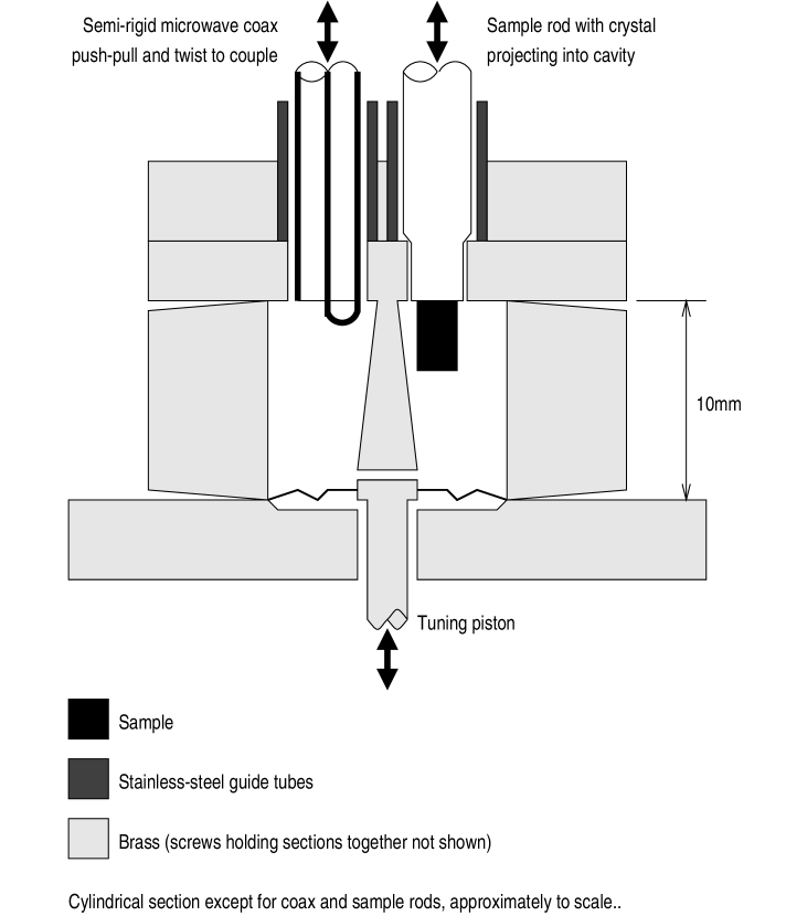
Figure 4.14: Schematic section through the tunable quarter-wave coaxial resonator used for frequency modulated CW NMR. The design shown allows top-loading of the sample, alternatively the sample may be glued directly to the central conductor.

A similar resonator was used for the field modulation experiments and is shown in figure 4.15. The internal dimensions are the same but the wall of the barrel section was made much thinner and a superconducting modulation coil wound around it. Figure 4.16 is a photograph of this resonator complete with brass base and support rods. The rod to the left of the photograph, with a brass coupling section, moves the tuning piston via a screw drive and a lever in the base. The stainless steel pipes brazed into the top of the resonator are guide pipes for the microwave coax and for the sample rod (one can be seen in the photograph, the other is obscured by the support rod in the foreground). All the stainless steel tubes are non-magnetic.

 

 

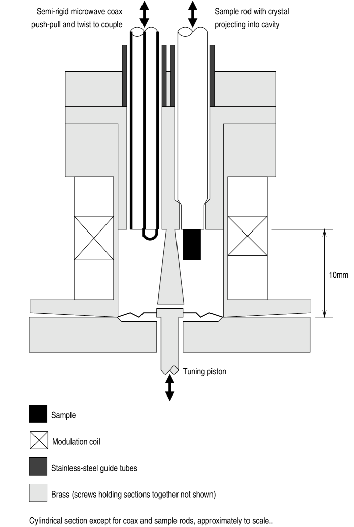
Figure 4.15: Schematic section through the tunable quarter-wave coaxial resonator used for field modulated CW NMR. The design shown allows top-loading of the sample, alternatively the sample may be glued directly to the central conductor.

4.5.1 Field modulation coil

In designing the modulation coil, eddy currents induced in the brass former/resonator were the main consideration. Eddy currents not only result in heating, they also reduce the field inside the resonator. For effective field modulation it was estimated that $\sim$1–10 mT amplitude would be required at the sample.

 

 

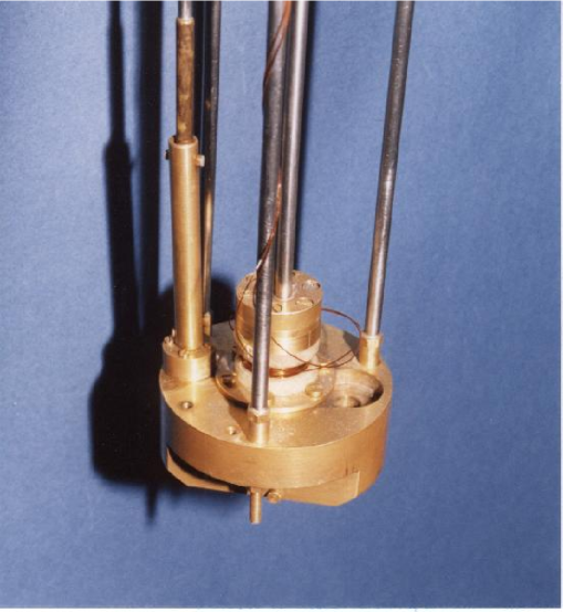
Figure 4.16: Photograph of the resonator with field modulation coil. The brass base section is $\approx$70 mm in diameter.

The strategy adopted was to minimise the physical size of the modulation coil by winding it directly onto a thin-walled brass resonator. The dimensions of the resonator are determined by the resonance frequency required and by the need to allow access for the coupling loop and sample rod. The internal dimensions were chosen as 12 mm diameter by 10 mm long, the same as for the resonator without a modulation coil, but with 0.5 mm wall thickness. Taking the resistivity of brass as $\approx 4\times 10^{-8}$ $\Omega$m at 4.2 K, and assuming a $\approx 10$ mm length of the resonator wall to be linked by all the flux through the the coil, gives an expression for the average power dissipation due to eddy currents:

$$P_{eddy}\sim 2{\times 10^{-3}}\nu_{mod}^{2}\langle B_{mod}\rangle^{2},$$ (4.1)

where $P_{eddy}$ is the average power dissipation (W); $\nu_{mod}$ is the modulation frequency (Hz); and $\langle B_{mod}\rangle$ is the RMS of the modulation field (T). This is probably an underestimate because it does not allow for other metalwork in the vacinity, in particular the top and base-plate of the resonator. However, using equation 4.1 as an estimate, 10 mT RMS modulation at 10 Hz (or 1 mT at 100 Hz) gives $\sim 20$ $\mu$W power dissipation which is not significant. For 10 mT at 100 Hz the dissipation is $\sim 2$ mW which is significant, but not prohibitive. We calculated that a 5 mm long coil of 100 turns wound directly onto the former would produce $\sim 6.5$ mT/A at the sample.

The actual coil consists of 111 turns of 0.38 mm diameter ‘Niomax’ (TiNb in copper) wire. The wire has a critical field of $>8$ T, an important consideration as it is inside the bore of the main magnet. The estimated inductance of the coil was 230 $\mu$H without the former. Using this inductance, a modulation frequency of 100 Hz and a modulation current of 1 A rms the back emf is $\approx$0.15 V. A simple amplifier, using an operation amplifier with a complimentary darlington output stage, was built to provide up to $\pm$3 A drive for the modulation coil.

 

 

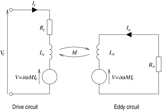
Figure 4.17: Equivalent circuit used to model the field modulation coil and induced currents in the former.

From the equivalent circuit shown in figure 4.17, we may write down an expression for the effective impedance of the modulation coil,

$$Z_{c}=R_{c}+\frac{\omega^{2}M^{2}R_{e}}{R_{e}^{2}+\omega^{2}L_{e}^{2}}+i\omega\left(L_{c}-\frac{\omega^{2}M^{2}L_{e}}{R_{e}^{2}+\omega^{2}L_{e}^{2}},\right),$$ (4.2)

where $R_{c}$, $L_{c}$, $R_{e}$ and $L_{e}$ are the resistances and inductances of the coil (drive) and eddy circuits respectively. The coupling between the circuits is modelled by the mutual inductance $M$. The values of $R_{e}$, $L_{e}$ and $M$ are not independent in terms of their effect on the impedance of the drive circuit. In order to parametrize equation 4.2 we make the substitutions

$$m=\frac{M^{2}}{R_{e}}\mbox{\hskip 28.45274pt and\hskip 28.45274pt}l=\frac{L_{e}}{R_{e}}.$$ (4.3)

The measured value of $R_{c}$, including the copper leads, was 66 m$\Omega$ with the resonator at 4.2 K. The coil itself was superconducting so this resistance is essentially that of the leads from the cryostat top-plate. Using the measured value of $R_{c}$, the parameters $L_{c}$, $m$ and $l$ were determined by fitting the magnitude and phase of $Z_{c}$ to experimental data from 20 Hz to 2 kHz. The fits are shown in figure 4.18: $L_{c}=1.24{\times 10^{-4}}$ H, $m=4.63{\times 10^{-8}}$ H${}^{2}/\Omega$ and $l=3.98{\times 10^{-4}}$ H$/\Omega$. The coupling $k_{M}$ between the drive and eddy cicuits is given by

$$k_{M}=\frac{L_{c}L_{e}}{M^{2}}=\frac{L_{c}l}{m^{2}}.$$ (4.4)

The parameters $L_{c}$, $m$ and $l$ are not very accurately determined from the fits; small changes in the fitting method or in the data points produce significantly different results. However, $k_{M}$ does appear to be reliably determined from the fits. From all fits, where the parameters varied by as much as 30 %, the result $k_{M}\approx 0.94$ was obtained with $<$1% variation. This confirms that the frequency modulation coil is strongly coupled to the eddy circuit, as expected for a coil wound onto a brass resonator.

 

 

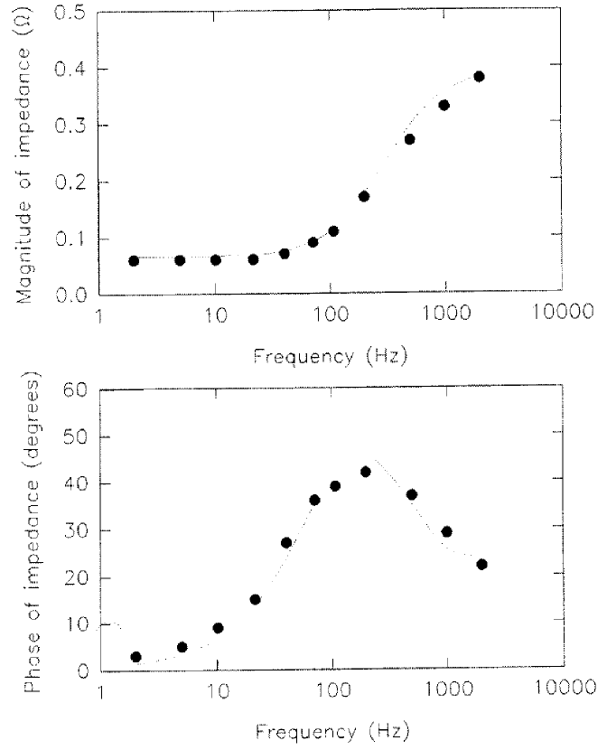
Figure 4.18: Phase and magnitude components of the modulation coil impedance. The points represent measured values and the line is a fit to the data.

The resonator for field modulation is a prototype. It should be possible to reduce the power dissipation significantly by thinning the barrel section further and reducing the amount of other metal in the vicinity. A better approach would be to use an insulating former, plated with gold on the inside. Also, the leads from the top of the cryostat to the coil ‘rattled’ at high drive currents. This could be simply fixed by taping the wires to one of the support rods.

4.5.2 Resonator frequency stability

At temperatures where the helium bath is superfluid ($T_{\lambda}\approx 2.19$ K) the frequency stability of the resonator is very good. Using the frequency locking loop to lock the oscillator frequency onto the resonance significantly improves on the stability of the oscillator alone. Typically, the frequency jitter is $<$20 kHz ($\approx$0.001 %) over a period of seconds. This is increased with large FM deviation ($>$5 MHz) but still remains $<$300 kHz. There is, however, a much larger long term drift, up to to $\approx$1 MHz per hour, and sometimes the frequency ‘jumps’, typically by 100–200 kHz. The drift is attributed to slow movement of the tuning components and the jumps are probably caused by knocking the apparatus. Jumps are more frequent when moving around close to the spectrometer than when it is left alone.

The formation of helium bubbles in the resonator was the most significant problem when working at 4.2 K. Various attempts were made to alleviate it: drilling holes in the top of the resonator to allow bubbles to escape, drilling holes in both the top and the bottom of the resonator, and working at low power. Drilling holes had very little effect, presumably because the resonator already has one or two fairly large holes in the top where the coaxial cable and sample rod fit loosly. Reducing the microwave power slows down bubble formation and reduces the frequency excursion (smaller bubbles) as shown in figure 4.19. The field modulation coil also heats the helium inside the resonator and causes similar behaviour. Modulation coil drive of 2 A rms and 0.1 mW microwave input produces bubbling similar to 0.5 mW microwave input alone (no field modulation).

 

 

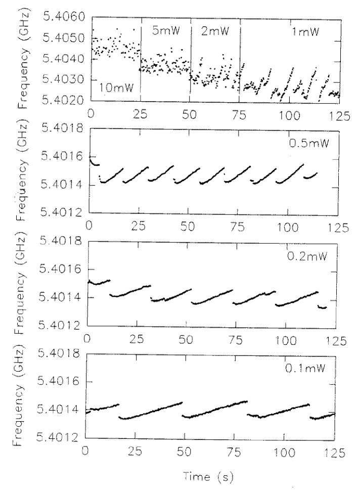
Figure 4.19: Graphs of resonator resonance frequency variation with time for various microwave input powers. The lower power traces clearly show the resonance frequency rise as a bubble forms, and then fall suddenly as it escapes.

The result of this bubbling was that it proved impossible to work with high power at 4.2 K. Typically, microwave powers of 1 mW or less were used. The bubbling disappears as the helium bath is cooled through the superfluid transition. Presumably there would be no bubbling problem in a continuous flow system where there is helium gas in the resonator. A similar design of resonator has worked with high stability when evacuated at nitrogen temperatures (on a test experiment using EPR of DPPH).

4.6 Cryogenics and magnet

Samples in resonant cells are suspended in the bore of a superconducting magnet at liquid helium temperatures. The magnet, magnet power supply (PS120A) and cryostat were supplied by Cryogenic Consultants Ltd. At 4.2 K the maximum field available is 8 T. By pumping on the helium bath containing both the magnet and the experimental resonator the temperature could be reduced to $\approx$1. 3 K with available pumps. Reducing the temperature to 1.5 K or less allows fields of up to 10 T to attained. Cooling the resonator and sample uses a significant proportion of the helium in the cryostat because the magnet is also cooled. The cryostat holds $\approx$21 l of helium, of which $\approx$2.5 l are required to cover the magnet (essential to avoid quenching). Cooling from 4.2 K down to 1.5 K uses $\approx$10 l and takes 2-3 hours. Fortunately, when cooled, the helium boil-off rate is not significantly greater than when at 4.2 K (0.3 l per hour with no current in the magnet leads and no microwave input). The magnet is equipped with a persistent-mode switch that allows a constant field to be maintained without any current in the magnet leads. At high fields this gives a significant reduction in the boil-off rate.

To find the sample temperature, the pressure above the helium bath is measured using a McLeod gauge. The temperature error is $\pm$0.05 K at 1.5 K, provided that localised sample heating is not significant. The field is determined by measuring the current through the magnet soleniod and using a field-current calibration supplied by the manufacturer. The field is homogeneous to within 0.18% in a cylinder of diameter 10 mm and height 10 mm at the centre of the solenoid.

4.7 Techniques

In this section we summarize experience of the successful field sweep technique, the unsuccessful frequency sweep technique, and results obtained ‘without’ modulation. Representative spectra from the field sweep technique can be found in chapter 5; none are given here.

4.7.1 Field sweeps

The field sweep technique works very well, principally because the frequency response of the microwave system, excluding the sample, is unaffected by the applied field. The sample may cause a shift in the resonant frequency of the resonator (section 4.7.3) but this is a relatively small and ‘smooth’ effect, and has not proved to be a problem.

We have obtained good NMR spectra from both field modulation and frequency modulation experiments. The principal advantage of field modulation is that the spectra have straightforward derivative character and it is thus easy to identify the centres of the NMR lines. Frequency modulation with third (or higher) harmonic detection gives more confusing line shapes. In some cases, it is the uncertainty in identifying the central feature of the line shape that dominates the measurement uncertainty. As expected, we found that no advantage was gained from using higher than third harmonic detection.

In order to sweep the field, the current in the superconducting magnet must be ramped up and down. This means that it is not possible to use the magnet in persistent mode, which imposes a penalty in terms of helium boil-off.

4.7.2 Frequency sweeps

Frequency swept systems require either a broadband transmission cell with the most level frequency response attainable; or a resonant cell whose resonant frequency is made to track that of the source, or conversely. The former method has been implemented by Cha [24] and, in this department, by Ross [67]. The latter strategy has been investigated as part of this work.

We have arranged the spectrometer so that the frequency of the microwave transmitter tracks the resonant frequency of the cell. Thus frequency sweeps can be performed by manual or motorized tuning the cell. Manual tuning causes far too much disturbance to the system, giving a background signal that is large, discontinuous and un-repeatable. Motorized tuning gives a much more repeatable background. In all attempts the background was much larger than any expected NMR signal. However, we note that the background was significantly reduced with field as opposed to frequency modulation. We conclude that this technique is inappropiate for systems where the transfer characteristics depend strongly on frequency.

4.7.3 Shift in the resonator frequency due to NMR

As part of this work we have detected NMR by the shift in the frequency of the combined resonator and sample resonance. This unusual detection method was feasible only because of the exceptionally large enhanced nuclear susceptibility of HoF₃.

In section 3.3.7, we have shown that in the regime where the resonator line width is much smaller than the NMR line width, the combined resonance frequency will respond to changes in the sample susceptibility. To a very good approximation, we expect a shift in frequency is proportional to $-\chi^{\prime}_{s}$, the dispersive part of the transverse RF susceptibility. The shift does not depend on the resonator $Q$ but the frequency stability of the system is improved by high $Q$ so, overall, the technique benfits from high $Q$.

When performing initial field sweep experiments on HoF₃ the shift in resonator resonance frequency resulting from the field dependece of the differential electronic susceptibility was very large, $\approx 20$ MHz. This suggested that it might be possible to see NMR by monitoring the frequency of the ‘locked’ system. Figure 4.20 shows a partially resolved NMR spectrum obtained in this way. The data were taken at 4.2 K using a single crystal sample with the $a$ axis parallel to the field ($4.2\times 1.9\times 1.6$ mm). The resonator $Q$ was $\approx$ 2500 and the frequency jitter was less than 100 kHz.

We have fitted a 7-line holmium spectrum to the frequency shift data: the result is shown as the solid line in figure 4.20. The model has 7 parameters: the position of the central line, the quadrupole splitting (in field), the resonance amplitude (the same for all 7 lines), the line width (the same for all 7 lines), and 3 parameters to allow for a quadratic background. The fit does not reproduce the structure that can be seen in the experimental data. By constraining the line width in the model, it is possible to reproduce a similar structure to that of the experimental data. However, we have been unable to get accurate agreement. This is not unreasonable because we have calculated the transverse RF susceptibilty from the Bloch equations which assume a Lorentzian line shape. In HoF₃ the holmium resonances are inhomogeneously broadened and the resulting line shape is not Lorentzian.

Figure 4.21 illustrates how the simple model of 7 resonances can produce a structure similar to that of the experimental spectrum. The figure shows 7 individual dispersion curves and the sum which represents the expected frequency shift. The sum clearly shows structure similar to that the experimental frequency shift data.

Figure 4.20 also showns the DC reflected power as a function of the applied field. There is a significant change in the reflected power resulting from NMR absorption and some structure is evident. However, the overall shape is rather asymmetric and no attempt has been made to model it.

 

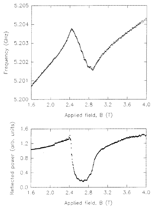
Loaded $Q\approx 2500$ (measured at 5.18 GHz).
Frequency modulation, $\pm$0.33 MHz at 50 kHz.
$T=4.2$ K.

 

Figure 4.20: NMR of holmium in HoF₃ seen by frequency shift of the resonator resonance (upper) and by DC power absorption (lower).

 

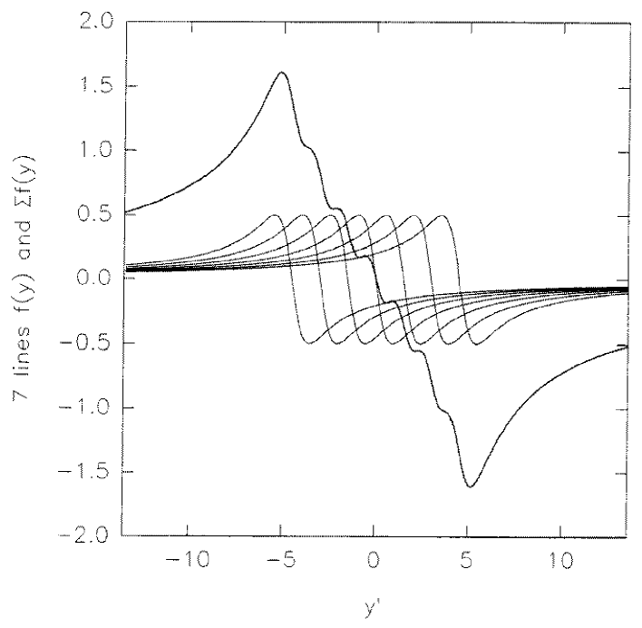
$$f(y)=\frac{-y}{1+y^{2}}$$

Seven lines from $y=y^{\prime}+1.5n$ where $n=-3,-2,-1,0,1,2,3$.

$${\textstyle\sum f(y)}=\sum_{n=-3}^{3}f(y^{\prime}+1.5n)$$

 

Figure 4.21: Form of resonator frequency shift predicted from the susceptibility change caused by holmium NMR. The 7 components resulting from the individual NMR lines are shown in conjuction with the resultant which is simply the sum of the component shifts.

Chapter 5 Holmium Trifluoride

This chapter is concerned with the low temperature magnetic and spectroscopic properties of HoF₃. The magnetic properties are dominated by the holmium ions and we use the Hamiltonian described in chapter 2 to model the ground $J$-manifold. HoF₃ orders antiferromagnetically at $T_{N}=0.53$ K [13] but here we consider only the paramagnetic phase. Although the term Van Vleck paramagnet is often applied to HoF₃, the susceptibility is not temperature independent [11]. This is because of the large nuclear contribution and the need to reduce the temperature below $\approx$2 K before thermal population effects become insignificant. Therefore it is probably more helpful to consider HoF₃ simply as a singlet electronic ground state system. In addition to magnetometry and NMR measurements on HoF₃, we have also made NMR measurements on holmium as a dilute substituent in YF₃: 1%Ho:YF₃.

The first part of this chapter surveys the crystal structure determinations for HoF₃ and YF₃ in the literature. From the structure some important properties that affect magnetic measurements are deduced. When discussing the structure we refer to the ‘holmium sites’ throughout. In the dilute material these will be mostly yttrium sites with occasional holmium occupancy.

Measurements of the electronic energy levels of the Ho³⁺ ions from several sources are compared with one another. Sharma et al [71] have determined crystal-field parameters from their measurements of the electronic energy levels, and we use these as the basis of our calculations.

We have studied the magnetization of HoF₃ for applied fields in the range 0–10 T along the principal crystallographic directions. The results show highly anisotropic magnetization, which accords with the earlier measurements of Bleaney et al [11]. The magnetization data are compared with calculations from the crystal-field parameters. Both pulsed and CW NMR have also been used to study HoF₃ and 1%Ho:YF₃. Whereas the magnetization measurements give thermal and spatial averages, the NMR frequencies reflect the properties of the ground state of the holmium ions. Thus, NMR provides a complementary test of the crystal-field parameters. We have also used the crystal-field parameters to calculate some properties that have not been measured, and suggest some potentially interesting experiments.

The samples studied in this work were prepared at the Clarendon Laboratory, Oxford. Methods of preparing rare-earth trifluorides are reviewed by Carlson and Schmidt [22]. The HoF₃ crystals are pale pink while the 1%Ho:YF₃ crystals are clear. Although we refer to the Ho in YF₃ crystals as 1%Ho, the concentration is nominal and not important to this work. We only require the holmium ions to be ‘dilute’ so that the dipolar and exchange fields are insignificant.

5.1 Crystal structure

The structure of rare-earth trifluorides was first studied by Zalkin and Templeton [78] using x-ray powder diffraction. They found TbF₃, DyF₃, HoF₃, ErF₃, TmF₃ and YbF₃ to be isostructural with YF₃. The unit cell is orthorhombic, space group P$n$m$a$ (D${}_{2h}^{16}$) and contains four formula units. Following convention, the unit cell axes are labelled $a$, $b$ and $c$ where the lengths are related by $b>a>c$. Table 5.1 gives the unit cell dimensions of YF₃, HoF₃ and TbF₃ [78]. The dimensions for HoF₃ and TbF₃ were verified by Piotrowski et al [57].

 
Compound Unit cell dimensions Unit cell volume $a$ (nm) $b$ (nm) $c$ (nm) ((nm)³) YF₃ 0.6353 0.6850 0.4393 0.1912 HoF₃ 0.6404 0.6875 0.4379 0.1928 TbF₃ 0.6513 0.6949 0.4384 0.1984  

Table 5.1: Unit cell dimensions of YF₃, HoF₃ and TbF₃ from powder x-ray diffraction.

Zalkin and Templeton [78] also found some of the trifluorides with the hexagonal LaF₃ structure but this is not confirmed in later work on HoF₃ and TbF₃ by Piotrowski et al [57]. Gries and Haschke [38] compare data from trifluorides with and without significant amounts of oxide fluorides and conclude that pure HoF₃, DyF₃ and TbF₃ exhibit only the P$n$m$a$ phase. The other rare-earth trifluorides and YF₃ exhibit different phases at high temperatures.

The volume per rare-earth ion in the trifluorides is $\approx$1.5 that in the rare-earth metals. In HoF₃ for example, the volume per holmium ion is 0.0482 (nm)³ (table 5.1) whereas in metallic holmium the volume per holmium ion is 0.0312 (nm)³ [32]. Thus the saturation magnetization of HoF₃ is $\approx$65% that of metallic holmium.

 
$\pm(r_{a},r_{b},r_{c})$ $\pm(\frac{1}{2}+r_{a},\frac{1}{2}-r_{b},\frac{1}{2}-r_{c})$ $\pm(-r_{a},\frac{1}{2}+r_{b},-r_{c})$ $\pm(\frac{1}{2}-r_{a},-r_{b},\frac{1}{2}+r_{c})$
The notation ($r_{a}$, $r_{b}$, $r_{c}$) is used in preference to the more usual ($x$,$y$,$z$) to avoid confusion with the coordinates used later.  

Table 5.2: Eightfold general ion positions in YF₃ and HoF₃ (space group P$n$m$a$), expressed as fractions of the unit cell dimensions.

The positions of the ions have been determined using x-ray diffraction by several workers. The eightfold general positions are given in table 5.2. The parameters $r_{a}$, $r_{b}$ and $r_{c}$ required to find the positions of the 4 rare-earth ions and 12 fluorine ions in the unit cell are given in table 5.3. Zalkin and Templeton [78] determined positions only for YF₃, noting that HoF₃ is isostructural with YF₃. The determinations of Bukvetskii and Garashina [16, 13] and of Piotrowski et al [57] were both for HoF₃. The two determinations for HoF₃ agree fairly well although no uncertainties are given by Piotrowski et al. There are some much larger differences between the HoF₃ and YF₃ determinations. In this work the positions determined by Bukvetskii and Garashina are used. The positions of the four holmium ions in the unit cell are given in table 5.4, together with the numerical labels which we use throughout this work. A unit cell is shown in figure 5.1.

 
Site & Zalkin¹ Piotrowski² Bukvetskii³ Ion symmetry Component YF₃ HoF₃ HoF₃ Y/Ho 4c (m) $r_{a}$ 0.367 0.367 0.3679(1) $r_{b}$ 0.25 0.25 0.25 $r_{c}$ 0.058 0.061 0.0614(1) F^′ 4c (m) $r_{a}$ 0.528 0.522 0.5224(9)⁴ $r_{b}$ 0.25 0.25 0.25 $r_{c}$ 0.601 0.584 0.5860(10)⁴ F^′′ 8d (1) $r_{a}$ 0.165 0.165 0.1662(6) $r_{b}$ 0.060 0.066 0.0645(6) $r_{c}$ 0.363 0.384 0.3797(9)
¹   Zalkin and Templeton [78].
²   Piotrowski et al [57].
³   Bukvetskii and Garashina [16], uncertainties in parenthesis.
⁴   Components transformed to conform with usual convention, ($r_{a}\rightarrow\frac{1}{2}+r_{a}$ and $r_{c}\rightarrow\frac{1}{2}-r_{c}$).  

Table 5.3: Ion positions in YF₃ and HoF₃ from powder x-ray data, expressed as fractions of the unit cell dimensions.

 
Ion Position in Position in Position in site $a$ direction† $b$ direction† $c$ direction† 0 0.3679 0.25 0.0614 1 0.6321 0.75 0.9386 2 0.8679 0.25 0.4386 3 0.1321 0.75 0.5614
†  Bukvetskii and Garashina [16].  

Table 5.4: Positions of the four holmium ions in the HoF₃ unit cell, expressed as fractions of the unit cell dimensions.

 

 

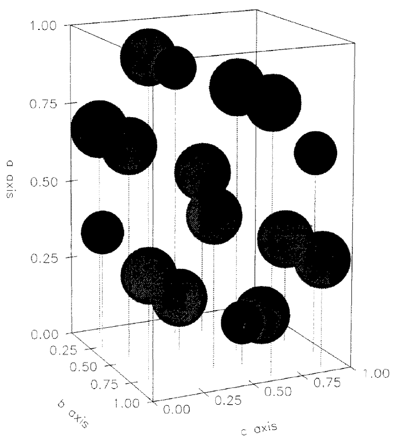
Figure 5.1: Ion positions in the HoF₃ unit cell with the axes marked in fractions of the lattice parameters: $a=0.6404$ nm, $b=0.6875$ nm and $c=0.4379$ nm. The filled (smaller) circles represent Ho³⁺ ions and the shaded circles represent F^- ions.

5.1.1 Holmium site symmetry

All four holmium sites in the HoF₃ unit cell have $C_{1h}$ symmetry. That is, the only symmetry element is a reflection plane which, in this case, is the $a$-$c$ plane. This makes the $b$ direction unique and it is convenient to identify it with the $z$ axis of the coordinate system ($x,y,z$) conventionally used to define crystal-field operators. Because the crystal axes are orthorhombic, we can conveniently adopt the correspondence $(x,y,z)\leftrightarrow(c,a,b)$; from now on we shall use the ($x,y,z$) system exclusively when discussing the holmium sites.

Reflection symmetry in the $x$-$y$ plane means that the lattice is invariant under the transformation $z\rightarrow-z$ relative to a holmium site. Thus, in any sum over the lattice, terms in $xz$ and $yz$ must vanish. In the case of a dipole sum this gives:

$$B_{xz}\equiv B_{zx}\equiv 0\mbox{\hskip 28.45274pt and\hskip 28.45274pt}B_{yz}\equiv B_{zy}\equiv 0,$$ (5.1)

where $B_{xz}$ means the component of the field in the $x$ direction due to moments in the $z$ direction, etc.. Similar considerations apply to the electric field gradient tensor:

$$V_{xz}\equiv V_{zx}\equiv 0\mbox{\hskip 28.45274pt and\hskip 28.45274pt}V_{yz}\equiv V_{zy}\equiv 0,$$ (5.2)

where $V_{xz}$ means $\frac{\partial^{2}V}{\partial z\partial x}$, etc.. The crystal-field parameters $B_{2}^{q}$ are related to the components of the electric field gradient tensor by

$$B_{2}^{0}\propto V_{zz}$$

$$B_{2}^{\pm 1}\propto(V_{xz}\pm iV_{yz})$$

$$B_{2}^{\pm 2}\propto(V_{xx}\pm iV_{yy}).$$ (5.3)

Thus the parameters $B_{2}^{\pm 1}$ and, in fact, all parameters $B_{k}^{q}$ ($k=2,4$ and 6) with odd $q$ vanish. This means that no more than 15 real parameters are required to specify the crystal-field interaction, whereas 27 would be required in the absence of reflection symmetry.

5.1.2 Holmium site inequivalence

Consideration of the holmium and fluorine ion positions in HoF₃ shows that each of the four holmium ions in the unit cell has different surroundings. However, the surroundings of the different sites are related by simple transformations. If we take holmium site 0 as a reference, the surroundings of site 1 differ by reflection in both the $x$-$z$ and $y$-$z$ planes. Similarly, the surroundings of site 2 differ by reflection in $y$-$z$ and the surroundings of site 3 differ by reflection in $x$-$z$.

Consider the interactions of the holmium ions with their surroundings, crystal-field and Zeeman (including dipolar and exchange). These interactions are unaffected by inversion of the surroundings with respect to the ionic coordinate system; or, equivalently, inversion of the ionic coordinate system with respect to the surroundings. The inversion symmetry of the electronic crystal-field interaction can be seen by noting that all terms are of even order in the components of $J$. We have already established that the surroundings of all four holmium sites are invariant under reflection in the $x$-$y$ plane. Combining this invariance with the coordinate inversion we see that the interactions will be unaffected by combined reflection in both the $x$-$z$ and $y$-$z$ planes (since an additional reflection in $x$-$y$ would complete an inversion of the surroundings). Hence, sites 0 and 1 are magnetically equivalent. Similarly, sites 2 and 3 are magnetically equivalent.

Now consider a magnetic field applied within the $x$-$z$ plane. The inequivalent site surroundings are related by reflection in the $x$-$z$ plane. The strengths of interactions on the ion are unaffected by the chirality of the surroundings, so although the response (the expectation value of $J_{y}$ for example) may differ in direction, the energy levels of the ion will be the same for both sites. Thus, for a field in the $x$-$z$ plane, the sites will be indistinguishable by any technique depends only on the ionic energy eigenvalues, as opposed to the eigenstates.

Similarly, we may consider a magnetic field applied within the $y$-$z$ plane and note that the inequivalent ion sites are alternatively related by reflection in the $y$-$z$ plane. Hence the sites will appear to be equivalent, in terms of the energy levels, if a field is applied in the $y$-$z$ plane. There is however, no symmetry argument to support site equivalence for a field applied in the $x$-$y$ plane or, indeed, for any field with non-vanishing $x$ and $y$ components. Furthermore, consideration of the dipolar or crystal fields leads us to conclude that the sites will be inequivalent for such a field.

5.1.3 Dipole sums

Bleaney et al [11] give the results of a dipole sum performed over a sphere of 3.0 nm radius about holmium site 0. Their results are obviously subject to some numerical errors as the sum of the diagonal terms $B_{xx}+B_{yy}+B_{zz}$ is not quite zero as required by Laplace’s equation (the discrepancy is $\approx$0.6% of the largest term). This cannot be explained by the imperfect convergence of the sum at 3.0 nm radius, because Laplace’s equation must hold for each term in the sum (see section 2.5.1).

Table 5.5 shows the dipole sum results of Bleaney et al [11] and of this work, both calculated using the ion positions given by Zalkin and Templeton [78]. The results are given in terms of the field at holmium site 0 due to a moment of 1 $\mu_{B}$ on the holmium ions at each of the other ion sites. If the sum is performed about the other holmium sites, then identical results are obtained for the diagonal terms ($B_{xx}$ etc.). For the cross term $B_{xy}$, the results for different sites are: -0.0022 T/$\mu_{B}$ at site 0 due to moments at site 1 (as in table 5.5), -0.0022 T/$\mu_{B}$ at site 1 due to moments at site 0, 0.0022 T/$\mu_{B}$ at site 2 due to moments at site 3, 0.0022 T/$\mu_{B}$ at site 3 due to moments at site 2 and zero for all other combinations. The terms $B_{xz}$ and $B_{yz}$ must vanish because of the site symmetry and the calculation does in fact give zero to the numerical accuracy of the computer program (rounding errors $<10^{-15}$ T/$\mu_{B}$).

We have also calculated the dipole sum using the ion positions of Bukvetskii and Garashina [16]. These results are compared with those obtained using the parameters of Zalkin and Templeton [78] in table 5.6. Although the different ion positions give slightly different results the two dipole sums are in good agreement. Figures 5.2 and 5.3 show how the dipole sum converges with increasing radius. The figures show the totals of the components at site 0 due to moments at all sites. Totals of the components at site 0 due to equal moments at all sites are given in tables 5.5 and 5.6. These must be treated with extreme caution because they are physically meaningless unless the moments on the holmium ions at all sites are the same.

 
Ion B_xx (T/$\mu_{B}$) B_yy (T/$\mu_{B}$) B_zz (T/$\mu_{B}$) B_xy (T/$\mu_{B}$) † ‡ † ‡ † ‡ † ‡ 0 0.0327 0.0330 -0.0135 -0.0133 -0.0192 -0.0195 0.0000 $<0.002$ 1 -0.0260 -0.0260 -0.0149 -0.0148 0.0408 0.0410 -0.0022 $<0.002$ 2 -0.0052 -0.0050 0.0642 0.0642 -0.0590 -0.0590 0.0000 $<0.002$ 3 -0.0115 -0.0118 -0.0214 -0.0212 0.0329 0.0330 0.0000 $<0.002$ total -0.0099 -0.0098 0.0144 0.0149 -0.0045 -0.0045 -0.0022 —
†  this work, summation over a sphere of 100 nm radius. The terms fluctuate by $<0.00001$ T/$\mu_{B}$ for radii between 50 nm and 100 nm.
‡  Bleaney et al [11], summation over a sphere of 3.0 nm radius.  

Table 5.5: Comparison of dipole sum results for holmium site 0 in HoF₃, calculated using the ion positions of Zalkin and Templeton.

 
Ion B_xx (T/$\mu_{B}$) B_yy (T/$\mu_{B}$) B_zz (T/$\mu_{B}$) B_xy (T/$\mu_{B}$) † ‡ † ‡ † ‡ † ‡ 0 0.0327 0.0327 -0.0135 -0.0135 -0.0192 -0.0192 0.0000 0.0000 1 -0.0260 -0.0258 -0.0149 -0.0152 0.0410 0.0410 -0.0022 -0.0023 2 -0.0052 -0.0057 0.0642 0.0649 -0.0590 -0.0592 0.0000 0.0000 3 -0.0115 -0.0115 -0.0214 -0.0211 0.0329 0.0327 0.0000 0.0000 total -0.0099 -0.0103 0.0144 0.0150 -0.0045 -0.0047 -0.0022 -0.0023
†  Ion positions of Zalkin and Templeton [78], summation over a sphere of radius 100 nm. The terms fluctuate by $<0.00001$ T/$\mu_{B}$ for radii between 50 nm and 100 nm.
‡  Ion positions of Bukvetskii and Garashina [16], summation over a sphere of radius 100 nm. The terms fluctuate by $<0.00001$ T/$\mu_{B}$ for radii between 50 nm and 100 nm.  

Table 5.6: Comparison of dipole sum results for holmium site 0 in HoF₃, calculated using the ion positions of Zalkin and Templeton and of Bukvetskii and Garashina.

 

 

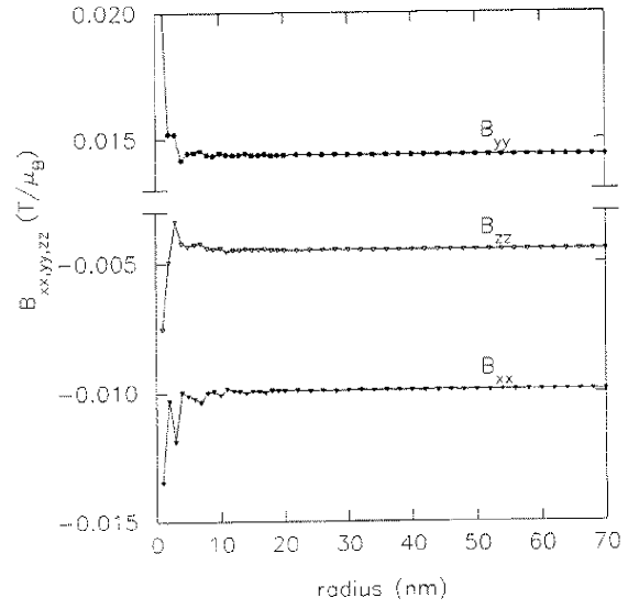
Figure 5.2: Graph showing diagonal components of the dipole sum as a function of the radius of the sphere over which the summation was performed.

 

 

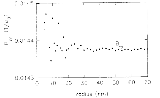
Figure 5.3: Enlarged graph to show convergence of the $B_{aa}$ component of the dipole sum with increasing radius of the sphere over which the summation was performed.

5.2 Determinations of the electronic energy levels

There are no complete determinations of the electronic levels of the ground ${}^{5}I_{8}$ manifold of Ho³⁺ in HoF₃. Sharma et al [71] studied HoF₃ by optical spectroscopy and measured transitions from the ground multiplet ${}^{5}I_{8}$ to the excited multiplets ${}^{5}G_{4}$ and ${}^{3}K_{8}$. From the transitions Sharma et al determined the separation of the positions of the first two excited levels relative to the ground level. Using these levels and the 26 levels in the ${}^{5}G_{4}$ and ${}^{3}K_{8}$ excited multiplets they obtained a set of crystal field parameters by least-squares fitting (see section 5.3). The measured levels and those calculated from the crystal field parameters are given in table 5.7. The calculated values are given in both cm^-1 and K units for comparison with optical and heat capacity results.

 
Sharma et al¹ Kraus et al² Bleaney et al³ Crystal field calculation (cm^-1) (cm^-1) (cm^-1) (cm^-1) (K) 0.00 0.00 0.00 0.00 0.00 5.90 – 6.59 6.86 9.87 37.99 38 – 42.96 61.81 – 81.5 – 93.45 134.46 – 105 – 96.65 139.06 – 165 – 174.72 251.39 – – – 180.53 259.75 – 170 – 193.43 278.32 – – – 217.95 313.59 – – – 242.21 348.49 – 253 – 242.76 349.28 – – – 264.23 380.94 – – – 275.67 396.63 – – – 281.44 404.94 – 358 – 350.89 504.86 – – – 370.58 533.19 – 401 – 377.27 542.82
¹   Sharma et al [71] from optical spectroscopy at temperatures from 1.6 K to 40 K.
²   Kraus et al [47] from Raman and infrared transmission spectroscopy, T$\approx$2 K.
³   Bleaney et al [11] from optical spectroscopy at temperatures from 1.5 K to 4.2 K.  

Table 5.7: Electronic energy levels of the ${}^{5}I_{8}$ ground manifold of Ho³⁺ in HoF₃

Sharma et al [71] quote an uncertainty of $<0.1$ cm^-1 on their level measurements. The measurements were made over the range 1.6 K to 40 K; those at temperatures above 1.6 K were used to identify the first two excited levels of the ${}^{5}I_{8}$ manifold by considering population effects.

Kraus et al [47] report several levels in the ground manifold, determined by infrared and Raman spectroscopy at 2 K. They suggest that agreement with the levels calculated using the crystal field parameters of Sharma et al [71] is acceptable for all but the level at 105 cm^-1. Both sets are given in table 5.7. Bleaney et al [11] report a splitting of 6.59 cm^-1 between the ground and first excited states, measured by optical spectroscopy between 1.4 K and 4.2 K. The same work reports heat capacity measurements that show a Schottky-type anomaly with a maximum at $\approx$3.5 K. This fits fairly well with a separation of 5.90 cm^-1 which should give a peak at 3.4 K. A separation of 6.59 cm^-1 should give a peak at 3.8 K, not in good agreement with the observed value. Bleaney et al note that the analysis is complicated by a steeply rising lattice contribution. However, that would only shift the observed peak to a higher temperature and so cannot explain the lower temperature of the observed peak. At the temperature of the observed peak the contribution to the specific heat resulting from the second excited state at 38 cm^-1 ($\approx$55 K) is less than $2\times 10^{-5}$ of the contribution from the first excited state, so that cannot explain the discrepancy either.

5.3 Crystal field

Sharma et al [71] obtained crystal-field parameters by fitting to the electronic energy levels measured in zero field (section 5.2). Corrections to the parameters are given by Ram and Sharma [65] and the corrected parameters are reproduced in table 5.8. Sharma et al and Ram and Sharma use the WYBOURNE convention. The parameters have been converted to MORRISON form which is more convenient when considering coordinate rotations. Details of these conversions are given in Appendix A.

 
Sharma et al† Sharma et al‡ (WYBOURNE form) (MORRISON form) (cm^-1) (K) (K) $B^{2}_{0}$ 78.5 112.95 $B^{2}_{0}$ 112.95 $B^{2}_{2}$ -199.6 -287.18 $\mbox{Re}(B^{2}_{2})$ -287.18 $B^{2}_{-2}$ 272.7 392.36 $\mbox{Im}(B^{2}_{2})$ -392.36 $B^{4}_{0}$ 17.9 25.75 $B^{4}_{0}$ 25.75 $B^{4}_{2}$ -101.7 -146.33 $\mbox{Re}(B^{4}_{2})$ -146.33 $B^{4}_{-2}$ -33.4 -48.06 $\mbox{Im}(B^{4}_{2})$ 48.06 $B^{4}_{4}$ 265.8 382.43 $\mbox{Re}(B^{4}_{4})$ 382.43 $B^{4}_{-4}$ -95.9 -137.98 $\mbox{Im}(B^{4}_{4})$ 137.98 $B^{6}_{0}$ 224.6 323.15 $B^{6}_{0}$ 323.15 $B^{6}_{2}$ 156.6 225.32 $\mbox{Re}(B^{6}_{2})$ 225.32 $B^{6}_{-2}$ -552.3 -794.65 $\mbox{Im}(B^{6}_{2})$ 794.65 $B^{6}_{4}$ 58.1 83.59 $\mbox{Re}(B^{6}_{4})$ 83.59 $B^{6}_{-4}$ -48.12 -69.24 $\mbox{Im}(B^{6}_{4})$ 69.24 $B^{6}_{6}$ -405.9 -584.01 $\mbox{Re}(B^{6}_{6})$ -584.01 $B^{6}_{-6}$ 31.3 45.03 $\mbox{Im}(B^{6}_{6})$ -45.03
†  Sharma et al [71] from fitting to electronic energy levels determined by optical spectroscopy.
‡  As †, but convention changed to MORRISON so that coordinate rotations can be calculated easily. Crystal-field parameter conventions are discussed in appendix A, coordinate rotations are discussed in appendix B.  

Table 5.8: Crystal field parameters for HoF₃.

Sharma et al [71] give a second set of parameters related by $30{{}^{\circ}}$ rotation about the $z$ axis. Subject to the corrections of Ram and Sharma [65], the two sets have been verified to transform into each other by $\pm 30{{}^{\circ}}$ rotations, to the precision given. Both sets have an rms deviation of 2.5 cm^-1 from the experimental data.

At a site of $C_{1h}$ symmetry, reflection in the $y$-$z$ plane is equivalent to a rotation of $180{{}^{\circ}}$ about the $y$ axis. The rotation can be represented by reflections in the $y$-$z$ and $x$-$y$ planes, but the lattice is invariant under reflection in $x$-$y$ plane so the rotation is simply equivalent to reflection in the $y$-$z$ plane. In the notation of appendix B, a rotation of $180{{}^{\circ}}$ about $y$ is represented by ${\sf D}(0,\pi,0)\equiv{\sf d}(\pi)$. Equation B.13 gives

$${\sf d}_{q^{\prime}-q}^{(k)}(\pi)=(-1)^{k-q^{\prime}}{\sf d}_{q^{\prime}q}^{(k)}(0),$$ (5.4)

and noting that ${\sf d}^{(k)}_{q^{\prime}q}(0)\equiv\delta_{q^{\prime}q}$, this simplifies to

$${\sf d}_{q^{\prime}-q}^{(k)}(\pi)=(-1)^{k-q^{\prime}}\delta_{q^{\prime}q}.$$ (5.5)

With crystal field parameters $M_{q}^{k}$ in MORRISON form (see appendix A), the transformed parameters $M^{\prime k}_{q}$ are given by equation B.5:

$$M^{\prime k}_{q}=\sum_{q^{\prime}=-k}^{k}{\sf D}_{qq^{\prime}}^{(k)}(0,\pi,0)M_{q^{\prime}}^{k}.$$ (5.6)

This simplifies to

$$M^{\prime k}_{q}=(-1)^{k-q}M_{-q}^{k},$$ (5.7)

and we note that $M^{k}_{-q}=(-1)^{q}(M_{q}^{k})^{\ast}$ (see section A.4). Also, $(-1)^{k}=1$ as $k$ is even and the final transformation is

$$M^{\prime k}_{q}=(M_{q}^{k})^{\ast}.$$ (5.8)

Rotation of $180{{}^{\circ}}$ about the $x$ axis is represented by ${\sf D}(-\frac{\pi}{2},\pi,\frac{\pi}{2})$. Combining equations 5.8 and B.9 gives an expression for the transformed parameters $M^{\prime\prime k}_{q}$:

$$M^{\prime\prime k}_{q} = e^{iq\frac{\pi}{2}}(M_{q}^{k})^{\ast}e^{-iq\frac{\pi}{2}}$$ (5.9)

$$= (M_{q}^{k})^{\ast}.$$ (5.10)

Rotation of $180{{}^{\circ}}$ about both the $x$ and $y$ axes is equivalent to the reflections in the $y$-$z$ and $x$-$z$ planes. In $C_{1h}$ symmetry this transformation leaves the parameters unchanged:

$$M^{\prime\prime\prime k}_{q}=((M^{k}_{q})^{\ast})^{\ast}=M^{k}_{q}.$$ (5.11)

We have now established the transformations required to find the crystal field parameters for all four holmium sites, given a set a parameters for one. Most importantly we see that although there are four sites, there are only two sets of crystal field parameters. Specifically, sites 0 and 1 have the same crystal field parameters (say $M^{k}_{q}$ for site 0 and thus $M^{\prime\prime\prime k}_{q}=M^{k}_{q}$ for site 1); sites 2 and 3 share a related set of parameters ($M^{\prime k}_{q}=M^{\prime\prime k}_{q}=(M^{k}_{q})^{*}$). This accords with the argument given in section 5.1.2.

5.4 Magnetometry

We have made magnetometry measurements on HoF₃ at 5 K with magnetic fields applied parallel to the principal crystallographic directions. These measurements were made using the Manchester vibrating sample magnetometer (VSM) with applied fields in the range 0 to 10 T. The temperature of 5 K was chosen as the lowest easily attainable with the continuous-flow cooling system. We estimate the sample temperature to have been within $\pm 1$ K of 5 K, and the crystal alignment to have been within $5{{}^{\circ}}$ of the nominal directions.

The dimensions of the crystal were 3.2$\times$1.98$\times$1.66 mm parallel to the $a$, $b$ and $c$ directions respectively, and the mass was 74.8$\pm$0.1 mg. The magnetization data have been scaled to give the moment per holmium ion and are shown in figure 5.4.

 

 

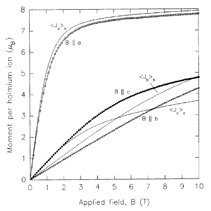
Figure 5.4: Magnetization curves for a HoF₃ crystal with the field applied parallel to the $a$, $b$ and $c$ axes. Magnetization is given in terms of the moment per holmium ion parallel to the applied field. The symbols represent magnetometry measurements and the lines are calculated from the crystal-field parameters. The calculated expectation values have been scaled by $g_{j}=1.2417$. The experimental data were taken with the sample at 5 K.

From the data in figure 5.4, the susceptibilities in vanishing applied field are 6.0, 0.48 and 0.88 $\mu_{B}$ atom^-1 T^-1 for fields along the $a$, $b$ and $c$ axes respectively. By extrapolating the data of Bleaney et al [11] to 5 K, the $a$ axis susceptibility is $\approx 6.7$ $\mu_{B}$ atom^-1 T^-1. Agreement is satisfactory given that the uncertainty in the temperature of the sample is $\pm 1$ K.

 

 

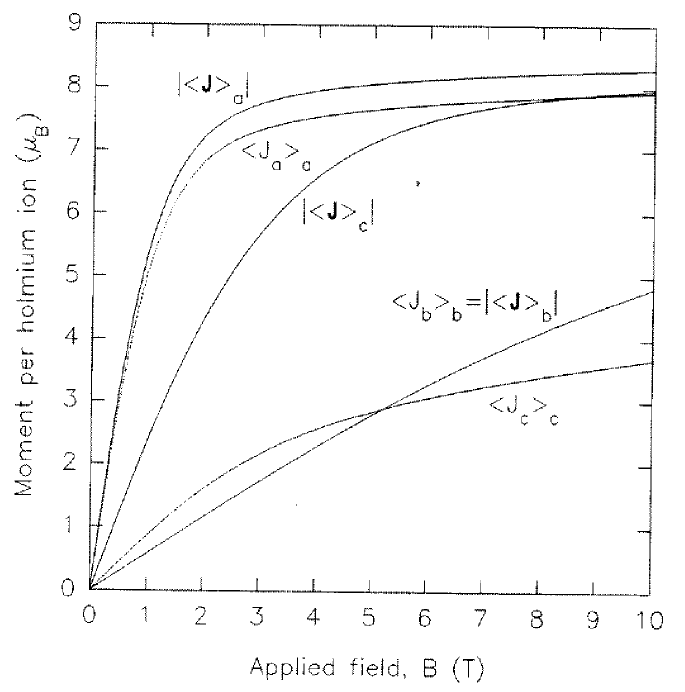
Figure 5.5: Magnetic moment per holmium ion calculated for fields applied along the principal crystallographic directions. For each direction the magnitude of the moment and the magnitude of the moment parallel to the field are plotted. In the case of the field parallel to the $b$-axis, these are identical as is expected from the site symmetry. The data shown are thermal averages calculated for $T=5$ K.

Figure 5.5 shows expectation value of the ionic moment calculated from the magnetization data and the results of crystal-field calculations for each of the principal crystallographic directions. The calculations and parameters used are discussed in section 5.4.1. Here we use the notation $\langle J_{r}\rangle_{s}$ for the expectation value of $J_{r}$ when the applied field is along the $s$ direction, and $\langle{\mbox{\boldmath$J$}}\rangle_{s}$ for the expectation value of $J$ when the field is applied along the $s$ direction. Thus, $\mid\langle{\mbox{\boldmath$J$}}\rangle_{s}\mid$ is the magnitude of the ionic moment for a field applied along the $s$ direction and $\langle J_{s}\rangle_{s}$ is the colinear component of the moment for a field applied along the $s$ direction.

The particularly striking feature of figure 5.5 is the difference between $\langle J_{c}\rangle_{c}$ and $\mid\langle{\mbox{\boldmath$J$}}\rangle_{c}\mid$. For 8 T applied along the $c$-axis, the calculation gives moments canted at $64{{}^{\circ}}$ to the field. The moments at sites 0 and 1 are canted in the opposite direction those at sites 2 and 3. The non-colinear part of the moment cancels when averaged over all four holmium sites so the bulk magnetization is determined by $\langle J_{c}\rangle_{c}$. Although not in good agreement with the magnetometry data, $\langle J_{c}\rangle_{c}$ is much closer to the measured value than $\mid\langle{\mbox{\boldmath$J$}}\rangle_{c}\mid$. The NMR frequencies, on the other hand, are determined by $\mid\langle{\mbox{\boldmath$J$}}\rangle_{c}\mid$. So, an NMR experiment with the field applied along the $c$ axis would provide an independent test of the crystal-field parameters.

Figure 5.5 shows the thermally averaged moments calculated for 5 K as would be measured by magnetometry. However, in rare-earth insulators at liquid helium temperatures we expect the NMR frequencies to be determined by the electronic ground state moment. For example, Bunbury et al [18] have shown this to be the case in Ho(OH)₃. In practice the values are very similar at moderate to high fields ($<0.4$ % difference between 5 K thermal average and ground state expectation values at 3 T) because only the ground state is appreciably populated.

5.4.1 Crystal-field calculations

Crystal-field calculations were performed using the parameter conversion and calculation programs described in Appendix C. We have used the crystal-field parameters of Sharma et al [71] (table 5.8), and the ionic parameters given in table 2.1. The data shown were calculated using a purely electronic Hamiltonian which makes the calculations very much faster because the Hamiltonian is only 17 by 17 rather than 136 by 136 if the nucleus is included. To check that the effect of the hyperfine interaction was not significant a few additional calculations using the combined electronic and nuclear Hamiltonian were also performed. They gave very similar results so we have confidence in the purely electronic calculations. We have neglected the dipolar and exchange interactions which give corrections of $<0.2$ T at the ion with 8 T applied along the $a$ axis. Such corrections do not significantly affect the agreement of the experimental and calculated data.

5.5 NMR

Bleaney et al [11] report field-swept NMR measurements on a ‘self-aligned’ sphere of HoF₃. By applying a 1.5 T field prior to the experiment the sphere was aligned with the crystallographic $a$-axis parallel to the field. At 3.52 GHz they found a spectrum with marginally resolved quadrupole structure (at $T=1.61$ K). The centre of their spectrum corresponds to an applied field of 0.559 T. To obtain the field experienced by the Ho ions, dipolar field and exchange field corrections were included. From their susceptibility measurements the moment per Ho ion is 5.01$\mu_{B}$ so, from the dipole sum, $B_{dip}=0.072$ T. The exchange field was estimated from susceptibility measurements, giving $B_{ex}=0.094$ T. This gives a total field at the ion of $B=0.725$ T.

From our crystal-field calculations (see section 5.5.3), we obtain an NMR spectrum centred at 3.145 GHz in a field of 0.725 T. This is about 12% lower than the frequency given by Bleaney et al [11]. To give the central line at 3.52 GHz from our crystal-field calculation would require an ionic field of 0.875 T, which suggests the need for better crystal-field parameters.

Bleaney et al [11] report a quadrupole splitting of 146(4) MHz which is in fair agreement with our calculated value of 132 MHz at 0.725 T. The quadrupole structure of their spectrum is only just resolved, with a line width of $\approx 0.04$ T. This line width in field corresponds to a line width in frequency of $\approx 130$ MHz (from the calculated ionic moment as a function of field). If the line width is assumed to be independent of frequency, then their observed line width disagrees with that of our NMR data, which was taken at higher fields and gives a significantly smaller line width in frequency. However, our data show very similar line widths for concentrated and dilute samples, suggesting that the dominant inhomogeneous broadening mechanism is crystal imperfection. If that is the case then we would expect the line width to be increased by the greater variation in quenching at low fields.

In this work we have used CW and pulsed NMR to study HoF₃ and 1%Ho:YF₃. The crystals have been both ‘self-aligned’ (HoF₃ only) and oriented with the applied field nominally along the $a$ direction. Most of the data have been taken by CW NMR with the sample and helium bath at 1.5 K to avoid frequency instability caused by helium bubbling. The pulsed NMR data have been used to confirm that certain features of the CW spectra are not instrumental artifacts.

5.5.1 Self-aligned sample

We have taken NMR spectra from a small, nearly spherical, HoF₃ sample that was allowed to move freely in the sample holder. By applying a field of 8 T the sample was aligned along the crystallographic $a$ axis (the easy direction).

Although the sample was only about 1 mm in diameter, reasonable spectra were obtained; a representative spectrum is shown in figure 5.6 (upper graph). This spectrum illustrates some of the problems of frequency modulation and third harmonic detection: there is a large background and the resonances are hard to interpret. The largest uncertainty in the resonance positions is due to resonance shape, and is estimated to be $\pm 0.05$ T. The lower graph of figure 5.6 shows that there is also a significant shift in the cavity resonance during the sweep, and some frequency instability toward the high field end of the sweep.

 

 

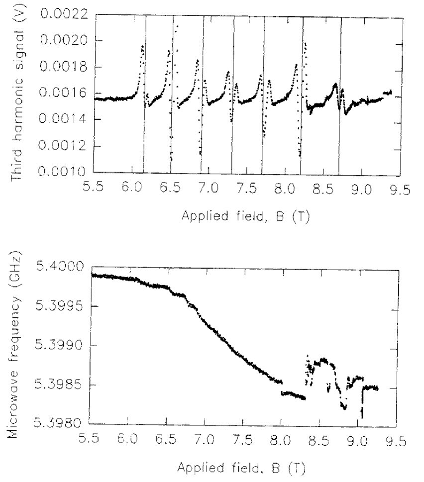
Figure 5.6: A 7 line holmium NMR spectrum from a small self-aligned HoF₃ sample. The vertical lines on the upper graph show the inferred line centres plotted to the nearest 0.05 T. The data were taken using frequency modulated CW NMR with third harmonic detection at 50 kHz, 1 mW incident microwave power, and $\pm 1.7$ MHz frequency modulation (considerably smaller than the NMR line width). The lower graph shows variation of the resonator frequency during the field sweep. The sample temperature was $1.5\pm 0.1$ K.

Figure 5.7 summarises the spectroscopic data. Between 4.95 GHz and 5.15 GHz it was not possible to resolve individual resonance lines so only the estimated centres of the spectra are plotted. The ‘collapse’ of the quadrupole splitting is attributed to the fact that the intra- and extra-ionic contributions to the quadrupole splitting, which have opposite signs, cancel each other at a field of the order of 2 T. The quadrupole splitting is predominantly extra-ionic at low fields and predominantly intro-ionic at high-fields.

 

 

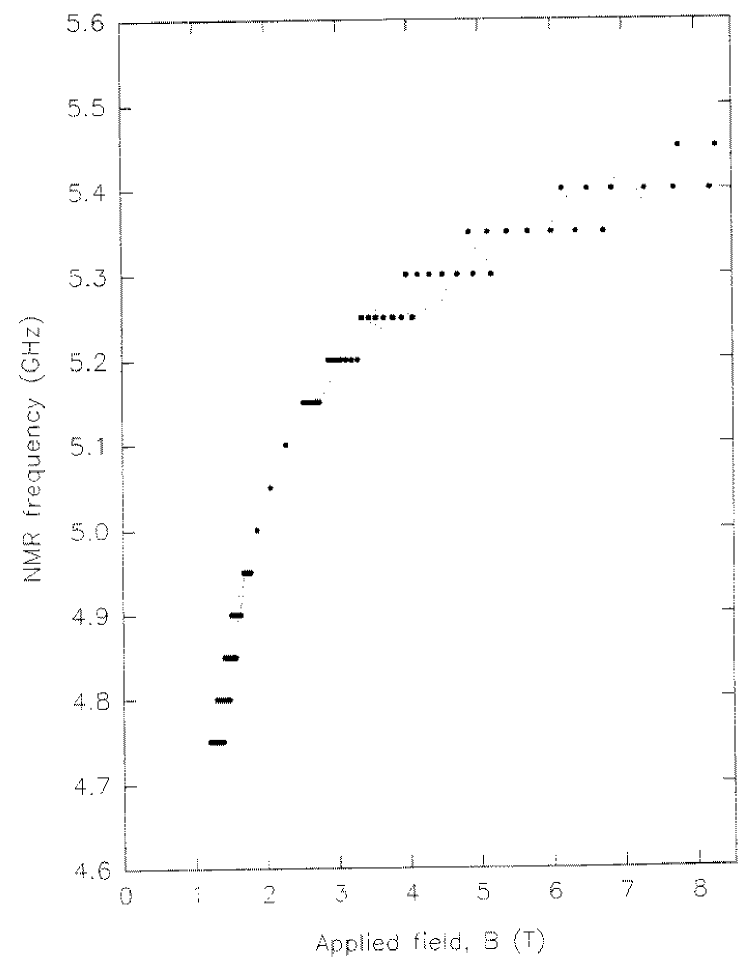
Figure 5.7: Graph showing NMR resonance frequencies against applied field for a self-aligned HoF₃ sample. Several sweeps were taken at some frequencies and in these cases the average resonance positions have been plotted. The data were taken using frequency modulated CW NMR and third harmonic detection. The sample temperature was $1.5\pm 0.1$ K.

5.5.2 Two spectra

All the NMR data except for those from the self-aligned sample show two distinct but overlapping spectra. Figure 5.8 shows two particularly well resolved spectra taken by frequency modulated CW NMR at high field. Figure 5.9 shows two marginally resolved spectra taken from the same sample using spin-echo NMR. That two spectra are seen by both the CW and pulsed NMR provides strong evidence that they are not an artefact of either technique. Although we have obtained resolved spectra from both CW and pulsed NMR, the resolution of our CW NMR data is superior. Since these spectra are obtained from the magnetically dilute sample (1%Ho:YF₃) we cannot attribute the presence of two spectra to different dipolar fields at different sites.

 

 

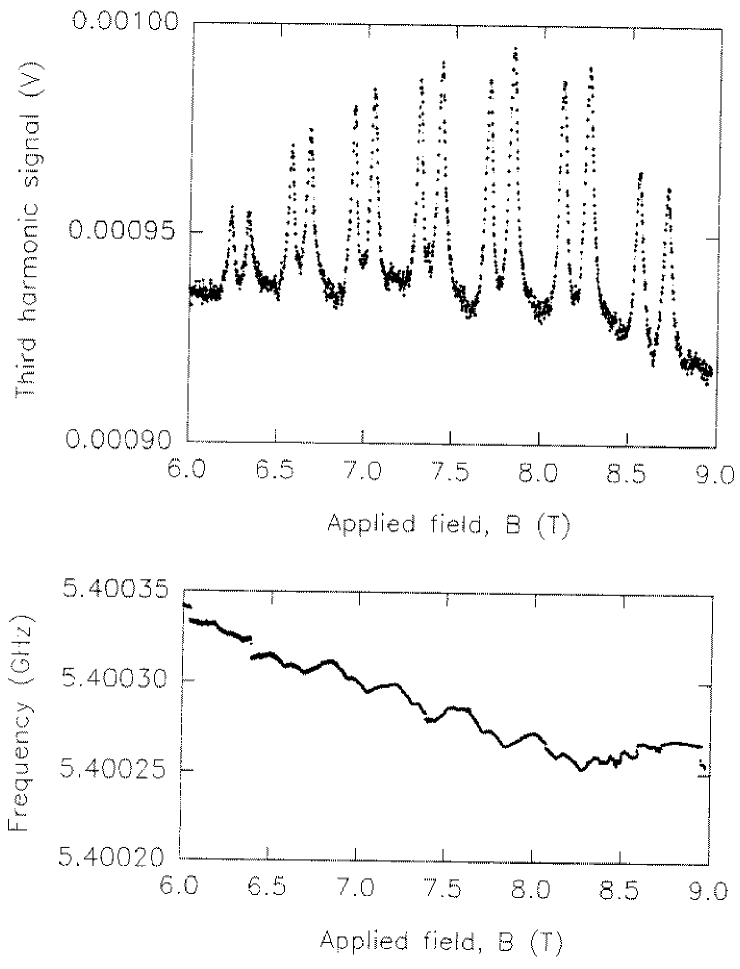
Figure 5.8: Two clearly resolved 7 line holmium spectra from 1%Ho:YF₃ (upper graph). The sample was aligned with the crystallographic $a$ axis nominally parallel to the applied field. The data were taken using frequency modulated CW NMR with third harmonic detection at 50 kHz, 1 mW incident microwave power, $\pm 1.7$ MHz frequency modulation, and loaded cavity $Q\approx 500$. The lower graph shows variation of the resonator frequency during the field sweep. The sample temperature was $1.5\pm 0.1$ K.

 

 

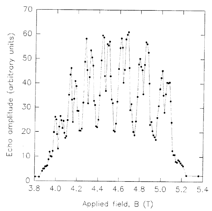
Figure 5.9: Two resolved 7 line holmium spectra from 1%Ho:YF₃ taken using spin-echo NMR at 5.300 GHz. The sample was aligned with the crystallographic $a$ axis nominally parallel to the applied field. The sample temperature was $1.5$ K.

Figure 5.10 shows three sets of resonance positions for 1%Ho:YF₃. Sets a) and b) were taken using frequency modulated CW NMR and set c) was taken using spin-echo NMR. The difference between sets a) and b) corresponds to a slight change in the orientation of the sample such that in set b) the two spectra are less well separated. The agreement of sets b) and c) (between which there was no mechanical movement) indicates that the effect is not an artefact of the CW technique. The uncertainties shown arise from the difficulty in locating the centres of the resonance lines.

 

 

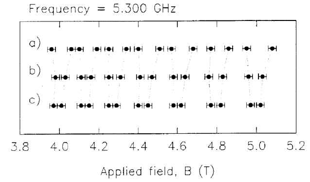
Figure 5.10: Graph showing the positions of the resonances in field for three successive NMR experiments performed at the same frequency and on the same sample. Between taking set a) and set b) the sample was removed and replaced. The frequency shifts are attributed to a small change in the orientation of the sample. The two experiments were otherwise performed under identical conditions. Set c) was taken by spin-echo NMR without moving the sample from set b). In all cases the frequency was $5.3000\pm 0.0005$ GHz and the sample temperature was $1.5\pm 0.1$ K.

The situation is confusing in some cases where there spectra appear to show 8 lines. This is attributed to there being two 7 line spectra shifted by an amount equal to the quadrupole splitting. Figure 5.11 shows one such spectrum, in this case taken by field modulated CW NMR for which the line shape is a simple derivative.

Figure 5.12 shows the calculated values of $\mid\langle{\mbox{\boldmath$J$}}\rangle\mid$ for a misaligned crystal. We consider the ground state only. The coordinate system is chosen such that $\theta=0{{}^{\circ}}$ corresponds to the $a$ axis and $\theta=90{{}^{\circ}}$, $\varphi=0{{}^{\circ}}$ corresponds to the $b$ axis. For a field applied along the $a$ axis ($\theta=0{{}^{\circ}}$), $\mid\langle{\mbox{\boldmath$J$}}\rangle\mid=6.6338$ and the sites are equivalent. This confirms invariance under he $C_{1h}$ symmetry operation, ie. reflection in the $a$-$c$ plane, which corresponds to $\varphi\rightarrow 180-\varphi$. Also, reflection in the $a$-$b$ plane exchanges sites 0 and 1 with sites 2 and 3, and corresponds to $\varphi\rightarrow-\varphi$. Taking $\theta=5{{}^{\circ}}$, the difference between the two sites is maximum for $\varphi=90{{}^{\circ}}$ and gives $\Delta_{sites}\mid\langle{\mbox{\boldmath$J$}}\rangle\mid=0.0085$ which is equivalent to $\Delta_{sites}B_{app}\approx 0.26~{}T$. This is larger than the observed field shift between any of the spectra. We may conclude that the observation of two distinct spectra is adequately explained by a misalignment of $<5{{}^{\circ}}$.

 

 

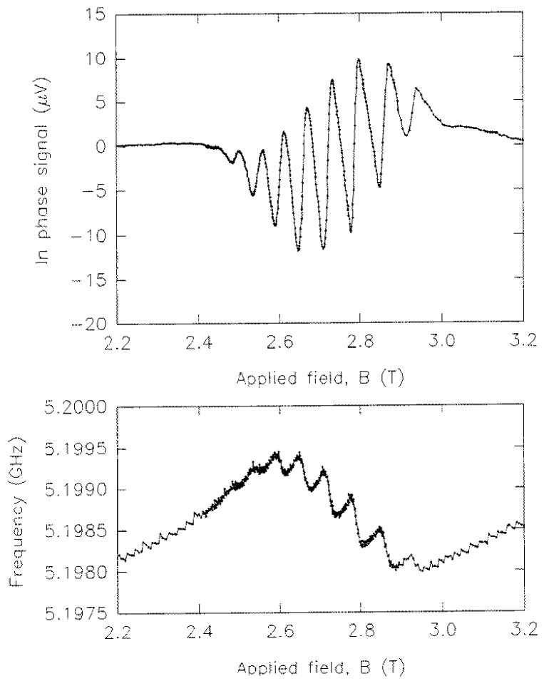
Figure 5.11: Graph showing an ‘8 line’ holmium spectrum. The two 7 line holmium spectra are shifted by an amount equal to the quadrupole splitting so there appears to be just a single 8 line spectrum. These data were taken by field modulated CW NMR. The modulation frequency was 107 Hz with $\pm 6$ mT deviation and 1 mW incident microwave power. A small frequency modulation at 100 kHz was used to track the resonator resonance; the sample temperature was 1.5 K.

 

 

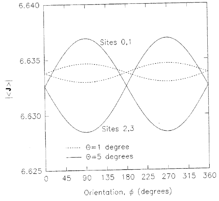
Figure 5.12: Graph showing the calculated variation of $\mid\langle{\mbox{\boldmath$J$}}\rangle\mid$ as a function of misalignment relative to the crystallographic $a$ direction. Curves are given for $\theta=1{{}^{\circ}}$ and $\theta=5{{}^{\circ}}$. In each case there are two curves: one for holmium sites 0 and 1, the other for sites 2 and 3. In the case $\theta=0{{}^{\circ}}$, $\varphi$ undefined and $\mid\langle{\mbox{\boldmath$J$}}\rangle\mid$ is slightly higher than the mean value for $\theta=1{{}^{\circ}}$.

5.5.3 Crystal-field calculations

Crystal-field calculations were performed use the parameter conversion and calculation programs described in Appendix C. As before, we have used the crystal-field parameters of Sharma et al [71] (table 5.8), and the electronic and nuclear parameters given in table 2.1. In particular, the extra-ionic quadrupole parameter $Q_{ext}=9.66\times 10^{-4}$ was derived from the ratio of the nuclear to electronic antishielding factors of Carboni [20] (table 5.8) for holmium ethylsulphate. (The nuclear and electronic antishielding factors vary considerably between different compounds and are not know for HoF₃.) We have used the ratio for holmium ethylsulphate because it gives reasonable agreement with the observed quadrupole splittings, much better than that for holmium hydroxide (also in table 2.1) for example. The collapse of the quadrupole splitting is particularly sensitive to the antishielding ratio. If there were better agreement between the experimental and calculated data, it would be possible to determine the ratio of antishielding factors for HoF₃ by fitting. However, given the discrepancy between the data and and the crystal-field calculation, we take the holmium ethylsulphate value as a reasonable first approximation to that for HoF₃.

Figure 5.13 summarizes our CW NMR data for 1%Ho:YF₃ and shows the NMR frequencies predicted from our crystal-field calculations. The dimensions of the crystal were 8.0 mm parallel to the $a$ direction and $2.0\times 1.8$ mm parallel to the $b$ and $c$ directions (order unknown). The sample was mounted with the $a$ direction nominally parallel to the applied field. Because the sample is magnetically dilute (1% holmium) we do not expect any significant corrections for dipolar field, exchange field or sample shape. It is thus reasonable to make direct comparison with calculated NMR frequencies shown in figure 5.13. Although the qualitative agreement is good, there are significant discrepancies. The experimental and calculated dipolar splittings differ by 2–3%, and the calculated quadrupole splittings are $\sim 20$% greater than the experimental values. However, we have already noted that the calculated quadrupole splittings depend strongly on the antishielding ratio, which is not known with any accuracy.

An interesting aspect of the collapse in the quadrupole splitting is that we observed spectra consisting of just two, partially resolved, lines between 5.0 and 5.1 GHz. We attribute the two lines to the two inequivalent sites, where the quadrupole structure within each is not resolved.

 

 

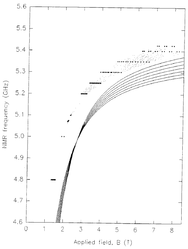
Figure 5.13: Graph showing NMR resonance frequencies against applied field for 1%Ho:YF₃. The points (joined with dotted lines as a guide to the eye) are experimental points, and the solid lines are from crystal-field calculation. The sample was oriented with the crystallographic $a$ axis nominally parallel to the applied field. The data were taken using frequency modulated CW NMR and third harmonic detection, The sample temperature was $1.5\pm 0.1$ K.

5.5.4 Dipolar and exchange fields

There is a significant difference between the spectra from the concentrated (HoF₃) and dilute (1%Ho:YF$3$) samples. We attribute this to the dipolar and exchange fields in the concentrated sample which will be negligible in the dilute sample. The difference is illustrated by figure 5.14 where the spectroscopic data from both samples is plotted together.

 

 

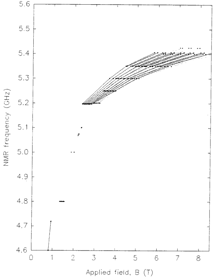
Figure 5.14: Graph showing NMR resonance spectra for both HoF₃ (‘concentrated’, solid lines) and 1%Ho:YF₃ (‘dilute’, dotted lines). All the data were take using frequency modulated CW NMR at $1.5\pm 0.1$ K.

In addition to the CW NMR data plotted in figure 5.14, C. Carboni of this department has made spin-echo measurements on the same HoF₃ sample. These are in good agreement with the results of this work. However, his data show only a single holmium spectrum which we attribute to better alignment of the $a$ axis with the applied field. The quadrupole splitting vanishes at 1.65 T and 5.05 GHz in the spin-echo data.

At 5.2GHz, the centre of the spectrum from the concentrated sample is about 0.45 T lower in field than the spectrum from the dilute sample. Assuming that both the exchange and dipolar fields are negligible in the dilute sample, we conclude that $B_{dip}+B_{ex}=0.45$ T in HoF₃ (under the stated conditions). In order to calculate $B_{dip}$, we take the ionic moment as 8.0 $\mu_{B}$, corresponding to the NMR frequency of 5.2 GHz. Ignoring a small cosine error ($<5$%) associated with the canted spin structure gives a bulk magnetization $M\approx 1.54\times 10^{6}$ Am-1. The dimensions of the crystal were $8.0\times 1.98\times 1.66$ mm parallel to the $a$, $b$ and $c$ directions respectively. Treating the crystal and an ellipsoid, with principal axes proportional to the dimensions, we obtain an estimated demagnetizing factor, $N\approx 0.065$, by interpolation from the tables of Cronemeyer [27]. We conclude that the Lorentz and demagnetization contributions to the dipolar field are $B_{L}+B_{dm}=(\frac{1}{3}-0.065)\mu_{0}M\approx 0.52$ T. Using the dipole sums given in section 2.5, with $B_{yy}=B_{aa}=0.015$ T$\mu_{B}^{-1}$ (see table 5.6), and ignoring effects due to canting, we estimate $B_{int}\approx 0.12$ T (the internal field or contribution to the dipolar field due to ions within the Lorentz sphere). Thus $B_{dip}\approx 0.64$ T and hence $B_{ex}=-0.19$ T. The fact that $B_{ex}$ is opposite and approximately equal to $B_{int}$ accords well with our observation that the NMR frequencies from the almost spherical (self-aligned) HoF₃ sample closely match those of the dilute material. However, our value for the exchange field does not agree with the results of Bleaney et al [11]. Scaling their value of $B_{ex}=0.094$ T for an ionic moment of 5.01 $\mu_{B}$ gives $B_{ex}\approx 0.15$ T for an ionic moment of 8.0 $\mu_{B}$. The origin of this discrepancy is unclear. It is unlikely that it can be explained by Bleaney’s neglect (and ours) of the effect of canting on the dipolar field.

5.5.5 Other predictions from the crystal-field parameters

We have made a set of crystal-field calculations for fields applied in the $a$-$c$ plane. The crystal-field axes were chosen such that the $b$-axis corresponds to $\theta=0{{}^{\circ}}$ and hence for $\theta=90{{}^{\circ}}$, $\varphi$ covers the $a$-$c$ plane. The ground-state values of ${\mid\langle{\mbox{\boldmath$J$}}\rangle\mid}$ are shown in figure 5.15 as a function of the field direction $\varphi$, where $\varphi=0{{}^{\circ}}$ corresponds to the field along the $c$ axis. The two curves represent the two different pairs of sites (the solid line for sites 0 and 1). This confirms that the calculation does not distinguish between the sites for fields along the $c$ and $a$ axes ($\varphi=0{{}^{\circ}}$ and $90{{}^{\circ}}$). We also see that the responses from the different sites are related by reflection in the $a$-$b$ plane ($\varphi\rightarrow-\varphi$) or the $c$-$b$ plane ($\varphi\rightarrow 180-\varphi$). However, the most striking features of figure 5.15 are the sharp dips in ${\mid\langle{\mbox{\boldmath$J$}}\rangle\mid}$ at $\varphi\approx 20{{}^{\circ}}$ and $160{{}^{\circ}}$. To find out whether this result is sensitive to the crystal-field parameters, several more calculations were performed with modified parameters. Qualitatively the results appears to be fairly insensitive to the parameters. For example, a similar dip is produced even if $M_{6}^{6}$ is set to zero. We have no experimental evidence for or against the behaviour predicted in figure 5.15.

 

 

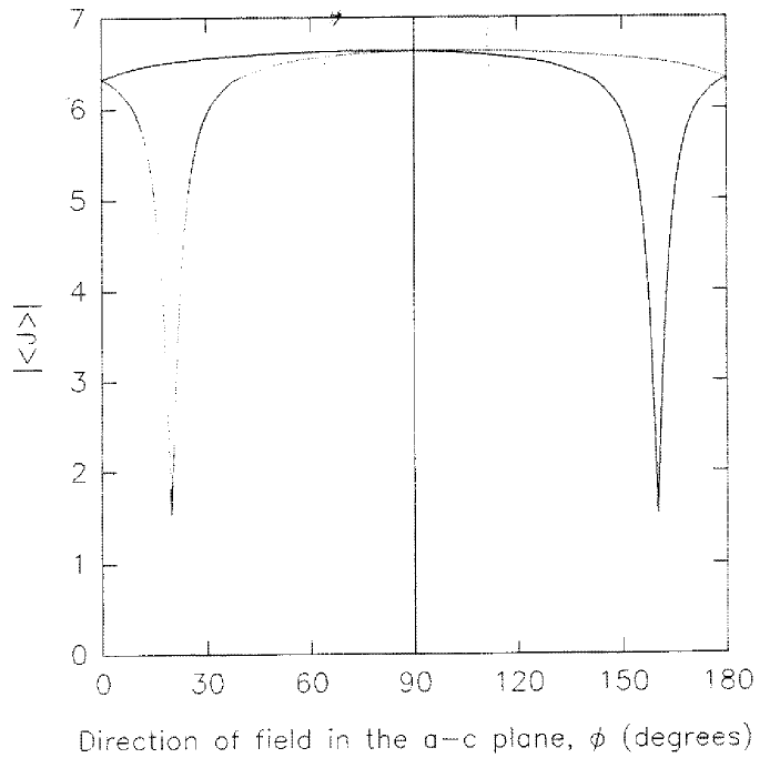
Figure 5.15: Magnitude of the ground state expectation value of $J$, ${\mid\langle{\mbox{\boldmath$J$}}\rangle\mid}$, as a function of the direction of the field of 8 T applied in the $a$-$c$ plane. The angle $\varphi$ covers the $a$-$c$ plane, and $\varphi=0{{}^{\circ}}$ corresponds to the field applied along the $c$ direction. The two lines are for the inequivalent holmium sites: one for sites 0 and 1, the other for sites 2 and 3.

It is interesting to note that our crystal-field calculations do not give the crystallographic $a$ axis as the easy axis for either site alone. This point is illustrated buy figure 5.15. However, the calculations do suggest that the $a$-axis should be the easy axis for a crystal composed of holmium with equal numbers of holmium ions on the two inequivalent sites. The ‘averaged’ easy axis is then in agreement with our experimental data and that of Bleaney et al [11].

5.5.6 Nuclear relaxation

From spin-echo measurements on 1%Ho:YF₃ taken at 5.300 GHz and 4.482 T we have estimated the spin-spin relaxation time to be $T_{2}=7\pm 2$ $\mu$s. For this we have assumed exponential relaxation which gives a fairly good fit to the experimental data. We have attempted to measure $T_{1}$, which turns out to be very long compared to that in other rare-earth insulators, such as the hydroxides. This caused problems because the pulse spectrometer has a maximum pulse separation if 1 s. However, by observing multiple stimulated echoes following a single spin-echo experiment, we estimate $T_{1}$ to be of the order of 2 s. No relaxation measurements were made on HoF₃.

5.6 Summary

From analysis of the crystal structure of HoF₃ we have deduced that the holmium sites are not magnetically equivalent, unless the applied field lies in either the $a$-$b$ or $b$-$c$ plane. The $a$ direction is the easy direction, and NMR results from a self-aligned HoF₃ show a single, well resolved, 7-line holmium spectrum. In support of our theoretical prediction that there are two magnetically inequivalent sites, we have NMR results which show two clearly resolved holmium spectra. However, these results are from samples aligned with the $a$ direction nominally parallel to the applied field. To reconcile the experimental results with our theoretical prediction, we have considered a small misalignment of the sample from the nominal $a$ direction. In section 5.5.2 we showed that a misalignment of $<5{{}^{\circ}}$ can give the observed separation between the two holmium spectra. Further supporting the idea of random misalignment we have shown different spectra from a single sample and taken in the same conditions except that the sample has been removed and replaced between experiments.

The crystal-field parameters of Sharma et al [71] provide good qualitative agreement with our NMR and magnetometry results. The quantitative agreement is fair, with a discrepancy of 2–3% between the calculated and measured dipolar splittings in 1%Ho:YF₃. This suggests the need for more accurate crystal-field parameters.

5.7 Further work

The most useful additional information would be a more accurate set of crystal-field parameters. These would be best derived from a set of electronic levels that included the complete ground manifold. The parameters of Sharma et al [71] are derived from the lowest 3 levels of the 17-level ground manifold and levels from excited multiplets. It is reasonable to expect that parameters derived from levels including more from the ground manifold would give a better descriptions of NMR and magnetometry measurements.

More spectroscopic information for the concentrated and dilute samples would allow a better analysis of the dipolar and exchange fields. The use of spherical samples would remove the need for demagnetizing field corrections which we have shown to be substantial. To test the predictions of out crystal-field calculations, an NMR experiment with the applied field along the $c$ axis would be interesting. The NMR frequencies would immediately support of disprove the prediction that the moments are strongly canted away from the $c$ axis. However, HoF₃ is clearly an extremely anisotropic system, so it is reasonable to expect that the transverse enhancement factor will be anisotropic. It may be that the enhancement factor is high for fields along the $a$ axis, which would help explain the strong signals seen in this work. But, it may be low in other directions making NMR more technically demanding. It would be desirable to use the crystal-field model to estimate enhancement factors for other directions before attempting NMR.

As part of this work, we have made several attempts to perform an NMR experiment with a HoF₃ sample mounted such that it could be rotated, putting the applied field anywhere in the $a$-$c$ plane. All attempts have failed either because of mechanical fouling of the rotation device, or because the crystal broke or shattered in an applied field. In spite of the technical difficulties, an investigation of either magnetization or NMR as a function of orientation of the field in the $a$-$c$ plane would be very useful. Our crystal field calculations predict ‘hard’ directions which could be checked by either technique. We also note that NMR with an applied field in the $a$-$c$ plane will, in general, give distinct spectra for the inequivalent holmium sites.

Chapter A Parameter conventions for crystal fields

There is a great deal of notational confusion in the literature on crystal fields. Much of the problem stems from the magnetism community, which has been concerned almost exclusively with the lowest $J$-manifold of rare-earth ions in situations of high symmetry. The simplicity of such systems has encouraged the use of ad hoc crystal-field parametrization schemes. These, though adequate for their immediate purpose, cannot be generalised in a consistent manner to situations of greater complexity. Conventions which are adequate to describe the lowest $J$-manifold of a system described by 2, 4 or even 6 crystal-field parameters tend to break down for low-symmetry systems, which may require up to 27 crystal-field parameters, especially if excited manifolds are to be included in the calculation. For these, a more coherent approach is required.

In this appendix we review the development of crystal-field notation, starting with the still widely used operator equivalents of Stevens [74]. Other commonly used notations are then described, followed by a brief note on computation using the 3-$j$ symbols. Finally, we present a detailed explanation of the inter-relationships of parameters in the notations described.

All notations discussed here use operators with symmetries related to those of the spherical harmonics. Parametrizing the interactions of $4f$ electrons with the crystal field using such operators is convenient because it is relatively easy to write down the matrix elements between the free-ion electron states used as a basis for calculations. If $B_{k}^{q}$ represents the coefficient of an operator related to the spherical harmonic $Y_{kq}$ (as defined in equation A.22) then the ranges of $k$ and $q$ are limited as follows (see, for example, [54]):

• For a $k^{th}$ order operator, $-k\leq q\leq k$.

• As $l=3$ for $4f$ electrons and only terms for which $k\leq 2l$ are required, $k\leq 6$.

• Time-reversal invariance requires $k$ to be even.

• To represent a real potential, $B_{k}^{-q}=(-1)^{q}(B_{k}^{q})^{\ast}$ which implies that the $B_{k}^{0}$ must be real and that we only need $(2k+1)$ real parameters for a given $k$.

• The $B_{0}^{0}$ term need not be included as it only produces a shift in all the energies, not a change in the splittings.

• Finally, all coefficients $B_{k}^{q}$ with $q\neq 0$ are subject to a phase factor which depends on the choice of $x$ and $y$ axes. If there are no crystallographic grounds to pick particular $x$ and $y$ axes, then the phase factor is usually chosen to set $\mbox{Im}(B_{2}^{1})$ or $\mbox{Im}(B_{2}^{2})$ to zero.

These conditions result in a maximum of 27 parameters (only 26 of which are independent: one may be set to zero by choice of axes) which may be expressed in terms of 3 real and 12 complex parameters:
$B_{2}^{0},B_{2}^{1},B_{2}^{2},$
$B_{4}^{0},B_{4}^{1},B_{4}^{2},B_{4}^{3},B_{4}^{4},$
$B_{6}^{0},B_{6}^{1},B_{6}^{2},B_{6}^{3},B_{6}^{4},B_{6}^{5}\mbox{ and }B_{6}^{6}.$
The $B_{k}^{0}$ are real and the $B_{k}^{q}$ ($q\neq 0$) are complex. Some notations use wholly real parameters by including $B_{k}^{q}$ for negative $q$ ($-k\leq q\leq k$) with operators related to the tesseral harmonics.

It is not usually the case that all of these parameters are required. The number of parameters is limited by the symmetry of the site of interest since the crystal-field Hamiltonian must be invariant under the operations of the symmetry group. However, the symmetry operations are tied to a set of axes so the number of parameters will depend on the choice of axes. For example, the surroundings of a site with $C_{1h}$ symmetry are invariant under reflection in the $x$-$y$ plane. If the $x$ and $y$ axes are not chosen to lie in this plane of reflection symmetry then, in general, 26 rather than 14 parameters will be required. The effect of the site symmetry is illustrated in table A.1, where the parameters required for all 32 point groups are listed.

 
Site symmetry† Class Crystal-field parameters required $O_{h}$, $T_{d}$, $O$, Cubic‡ $B_{4}^{0}$, $\mbox{Re}(B_{4}^{4})$, $B_{6}^{0}$, $\mbox{Re}(B_{6}^{4})$. $T_{h}$, $T$ $D_{6h}$, $D_{3h}$, $D_{6}$, $C_{3h}$, Hexagonal $B_{2}^{0}$, $B_{4}^{0}$, $B_{6}^{0}$, $\mbox{Re}(B_{6}^{6})$. $C_{6v}$, $C_{6h}$, $C_{6}$ $D_{4h}$, $D_{2d}$, $C_{4v}$, $D_{4}$ Tetragonal $B_{2}^{0}$, $B_{4}^{0}$, $\mbox{Re}(B_{4}^{4})$, $B_{6}^{0}$, $\mbox{Re}(B_{6}^{6})$. $D_{3}$, $D_{3d}$, $C_{3v}$ Trigonal $B_{2}^{0}$, $B_{4}^{0}$, $\mbox{Re}(B_{4}^{3})$, $B_{6}^{0}$, $\mbox{Re}(B_{6}^{3})$, $\mbox{Re}(B_{6}^{6})$. $C_{4}$, $C_{4h}$, $S_{4}$ Tetragonal $B_{2}^{0}$, $B_{4}^{0}$, $\mbox{Re}(B_{4}^{4})$, $B_{6}^{0}$, $B_{6}^{4}$. $C_{3}$, $S_{6}(C_{3i})$ Trigonal $B_{2}^{0}$, $B_{4}^{0}$, $\mbox{Re}(B_{4}^{3})$, $B_{6}^{0}$, $B_{6}^{3}$, $B_{6}^{6}$. $D_{2}$, $D_{2h}$, $C_{2v}$ Orthorhombic $B_{2}^{0}$, $\mbox{Re}(B_{2}^{2})$, $B_{4}^{0}$, $\mbox{Re}(B_{4}^{2})$, $\mbox{Re}(B_{4}^{4})$, $B_{6}^{0}$, $\mbox{Re}(B_{6}^{2})$, $\mbox{Re}(B_{6}^{4})$, $\mbox{Re}(B_{6}^{6})$. $C_{2}$, $C_{2h}$ Monoclinic $B_{2}^{0}$, $\mbox{Re}(B_{2}^{2})$, $C_{1h}\,(C_{s},C_{1v})$ $B_{4}^{0}$, $B_{4}^{2}$, $B_{4}^{4}$, $B_{6}^{0}$, $B_{6}^{2}$, $B_{6}^{4}$, $B_{6}^{6}$. $C_{1}$, $C_{i}$ Triclinic $B_{2}^{0}$, $\mbox{Re}(B_{2}^{1})$, $B_{2}^{2}$, $B_{4}^{0}$, $B_{4}^{1}$, $B_{4}^{2}$, $B_{4}^{3}$, $B_{4}^{4}$, $B_{6}^{0}$, $B_{6}^{1}$, $B_{6}^{2}$, $B_{6}^{3}$, $B_{6}^{4}$, $B_{6}^{5}$, $B_{6}^{6}$.
†  Point groups are used to describe the site symmetry, for an explanation of the labels see Sachs [69] for example.
‡  The four parameters for cubic symmetry are not all independent (see section A.3).
Parameters $B_{k}^{q}$ are complex for $q>0$, where only the real part is required it is written explicitly as $\mbox{Re}(B_{k}^{q})$. In this tabulation the phase factor determined by the orientation of the $x$ and $y$ axes is chosen to give the minimum number of parameters, for example in the triclinic class $B_{2}^{1}$ is made real. Tabulation after Walter [76].  

Table A.1: Parameters required to describe the crystal-field interaction in the 32 point group symmetries.

A.1 Stevens operator-equivalent notation

In Stevens’s original paper [74], four potential functions were considered. These are reproduced in table A.2; the summations remind us that crystal-field theory was based on the idea of independent electrons in a non-spherically symmetric potential.

 

$$V_{2}^{0}=\sum(3z^{2}-r^{2})$$

$$V_{4}^{0}=\sum(35z^{4}-30r^{2}z^{2}+3r^{4})$$

$$V_{6}^{0}=\sum(231z^{6}-315r^{2}z^{4}+105r^{4}z^{2}-5r^{6})$$

$$V_{6}^{6}=\sum(x^{6}-15x^{4}y^{2}+15x^{2}y^{4}-y^{6})$$

 

Table A.2: Potential functions considered by Stevens. Summations are over the coordinates of all electrons.

Each $V_{n}^{m}$ may be factorized and written in the form $f_{n}(r)Y_{n}^{m}(\theta,\varphi)$ so as to transform according to an irreducible representation of the rotation group. Stevens notes that there are simple relations between the matrix elements of potential operators and appropriate angular momentum operators inside a manifold of constant $J$ (a result that follows from the Wigner-Eckart theorem, see, for example, Brink and Satchler [12]). By comparing the matrix elements of the potential operators and of angular momentum operators, Stevens determined equivalent angular momentum operators. In generating such operator equivalents allowance must be made for the non-commutation of $J_{x}$, $J_{y}$ and $J_{z}$. Operator equivalents that have been symmetrized to allow for non-commutation are given and are reproduced in table A.3. The factors $\alpha$, $\beta$ and $\gamma$ are referred to as operator-equivalent coefficients and relate the angular momentum operators to the potential operators. Stevens [74] lists the values of the operator-equivalent coefficients ($\alpha$, $\beta$ and $\gamma$), together with the matrix elements of $V_{2}^{0}$, $V_{4}^{0}$ and $V_{6}^{0}$ for the ground manifolds of all the rare-earth ions (in the $L$-$S$ coupling scheme). Values of $\alpha$, $\beta$ and $\gamma$ corrected for intermediate coupling (a significant factor in many rare-earth ions) are also available: see, for example, Wybourne [77]. The factors $\langle r^{n}\rangle$ are expectation values of $r^{n}$ for the $4f$ electrons and thus depend on both the ion and the configuration. Freeman and Desclaux [37] tabulate values of $\langle r^{n}\rangle$ from relativistic calculation.

 

$$V_{2}^{0}\equiv\alpha\langle r^{2}\rangle[3J_{z}^{2}-J(J+1)]$$

$$V_{4}^{0}\equiv\beta\langle r^{4}\rangle[35J_{z}^{4}-30J(J+1)J_{z}^{2}+25J_{z}^{2}-6J(J+1)+3J^{2}(J+1)^{2}]$$

$$V_{6}^{0}\equiv\gamma\langle r^{6}\rangle[231J_{z}^{6}-315J(J+1)J_{z}^{4}+735J_{z}^{4}+105J^{2}(J+1)^{2}J_{z}^{2}-525J(J+1)J_{z}^{2}$$

$$\hskip 36.135pt+294J_{z}^{2}-5J^{3}(J+1)^{3}+40J^{2}(J+1)^{2}-60J(J+1)]$$

$$V_{6}^{6}\equiv\gamma\langle r^{6}\rangle\frac{1}{2}[(J_{x}+iJ_{y})^{6}+(J_{x}-iJ_{y})^{6}]$$

The expressions for $V_{2}^{0}$, $V_{4}^{0}$ and $V_{6}^{0}$ are due to Stevens [74]; that for $V_{6}^{6}$ is due to Elliott and Stevens [35].
 

Table A.3: Operator equivalents inside a manifold of constant $J$.

In applying Stevens’ method to cerium ethyl sulphate, Elliott and Stevens [33] give a more general expansion of the crystal-field potential in terms of spherical harmonics:

$$V_{cf}=\sum_{n=2,4,6}\sum_{m=0\ldots n}A_{n}^{m}\langle r^{n}\rangle Y_{n}^{m}(\theta,\varphi).$$ (A.1)

where the $A_{n}^{m}$ are numerical parameters and the $Y_{n}^{m}(\theta,\varphi)$ are spherical harmonics. In the case of $f$ electrons in $C_{3h}$ symmetry this is reduces the four terms discussed by Stevens [74] but Elliott and Stevens note that the $V_{6}^{6}$ term is a combination of $Y_{6}^{6}$ and $Y_{6}^{-6}$.

Elliott and Stevens [35] later considered $J$-mixing, the admixture of other $J$-manifolds by the crystal field. They calculated operator-equivalent coefficients between states with different total angular momenta, still however, assuming $L$-$S$ coupling. They also note similarities between the operator-equivalent coefficients and Racah’s coefficients [61] and give an expression for the operator equivalent of $V_{6}^{6}$ (table A.3). In a later paper [34] they tabulate the matrix elements of $V_{6}^{6}$. In order to extend crystal-field calculations to sites with $C_{3v}$ symmetry Judd [45] added operator equivalents for $V_{4}^{3}$ and $V_{6}^{3}$ together with tables of their matrix elements within a constant $J$ manifold.

A significant shift in notation was introduced by Baker, Bleaney and Hayes [4] (hereinafter referred to as BBH), who recast the crystal-field interaction in the form of an explicitly quantum-mechanical Hamiltonian, ${\cal H}_{c\!f}$:

$${\cal H}_{c\!f}=\sum_{n=2,4,6}\sum_{m=0\ldots n}{B_{n}^{m}}{O_{n}^{m}}$$ (A.2)

within a manifold of given $J$, where

$${B_{n}^{m}}=A_{n}^{m}\langle r^{n}\rangle\langle J\parallel\alpha_{n}\parallel J\rangle.$$ (A.3)

The operator-equivalent coefficients $\alpha$, $\beta$ and $\gamma$ are rewritten in the more general form $\langle J\parallel\alpha_{n}\parallel J\rangle$ where $n=2,4,6$ respectively. The $A_{n}^{m}$ are the same as those of equation A.1. The operator equivalents ${O_{n}^{m}}$ do not include the operator-equivalent coefficients or the radial factors $\langle r^{n}\rangle$. Both factors are included in the parameters $B_{n}^{m}$, which restricts application of the $B_{n}^{m}$ a single $J$-manifold. The parameters $A_{n}^{m}$ are (in principle) common to an entire $LS$-term. BBH tabulate the matrix elements of $O_{4}^{4}$ and $O_{6}^{4}$ for application to tetragonal symmetry. They also obtain a complete ‘spin Hamiltonian’ for the manifold by adding a Zeeman term to ${\cal H}_{c\!f}$. Using the same notation, Jones et al [44] tabulate the operator equivalents $O_{2}^{2}$, $O_{4}^{2}$ and $O_{6}^{2}$ and their matrix elements, thereby extending the notation to orthorhombic symmetry. Corrections to some of the matrix elements [34, 44, 74] are given by Hutchings [43]. A complete tabulation of ${O_{n}^{m}}$ for $n=2,4,6$ and $m=0,1\ldots n$ (equation A.2) is given by Orbach [55] and is reproduced in table A.4.

A similar notation is used by Scott [70] and by Abragam and Bleaney [1] (but they are not entirely consistent, sometimes using the BBH form). The difference is that the operator-equivalent coefficients, $\langle J\parallel{\alpha_{n}}\parallel J\rangle$, are not included in the crystal-field parameters. To avoid confusion with BBH, we use $S_{n}^{m}$ to denote the $A_{n}^{m}\langle r^{n}\rangle$ (the ‘${B_{n}^{m}}$’ of Scott [70]). Then, by equation A.3,

$$B_{n}^{m}=\langle J\parallel{\alpha_{n}}\parallel J\rangle S_{n}^{m}.$$ (A.4)

The crystal-field Hamiltonian may now be rewritten as

$${\cal H}_{c\!f}=\sum_{n=2,4,6}\sum_{m=0\ldots n}S_{n}^{m}\langle J\parallel{\alpha_{n}}\parallel J\rangle{O_{n}^{m}}.$$ (A.5)

 

$$O_{2}^{0}=3J_{z}^{2}-J(J+1)$$

$$O_{2}^{1}=\frac{1}{4}[J_{z}(J_{+}+J_{-})+(J_{+}+J_{-})J_{z}]$$

$$O_{2}^{2}=\frac{1}{2}[J_{+}^{2}+J_{-}^{2}]$$

$$O_{4}^{0}=35J_{z}^{4}-[30J(J+1)-25]J_{z}^{2}-6J(J+1)+3J^{2}(J+1)^{2}$$

$$O_{4}^{1}=\frac{1}{4}[(7J_{z}^{3}-3J(J+1)J_{z}-J_{z})(J_{+}+J_{-})+(J_{+}+J_{-})(7J_{z}^{3}-3J(J+1)J_{z}-J_{z})]$$

$$O_{4}^{2}=\frac{1}{4}[(7J_{z}^{2}-J(J+1)-5)(J_{+}^{2}+J_{-}^{2})+(J_{+}^{2}+J_{-}^{2})(7J_{z}^{2}-J(J+1)-5)]$$

$$O_{4}^{3}=\frac{1}{4}[J_{z}(J_{+}^{3}+J_{-}^{3})+(J_{+}^{3}+J_{-}^{3})J_{z}]$$

$$O_{4}^{4}=\frac{1}{2}[J_{+}^{4}+J_{-}^{4}]$$

$$O_{6}^{0}=231J_{z}^{6}-105[3J(J+1)-7]J_{z}^{4}+[105J^{2}(J+1)^{2}-525J(J+1)+294]J_{z}^{2}$$

$$\hskip 28.90755pt-5J^{3}(J+1)^{3}+40J^{2}(J+1)^{2}-60J(J+1)$$

$$O_{6}^{1}=\frac{1}{4}[(33J_{z}^{5}-(30J(J+1)-15)J_{z}^{3}+(5J^{2}(J+1)^{2}-10J(J+1)+12))J_{z}(J_{+}+J_{-})$$

$$\hskip 28.90755pt+(J_{+}+J_{-})(33J_{z}^{5}-(30J(J+1)-15)J_{z}^{3}+(5J^{2}(J+1)^{2}-10J(J+1)+12))J_{z}]$$

$$O_{6}^{2}=\frac{1}{4}[(33J_{z}^{4}-(18J(J+1)+123)J_{z}^{2}+J^{2}(J+1)^{2}+10J(J+1)+102)(J_{+}^{2}+J_{-}^{2})$$

$$\hskip 28.90755pt+(J_{+}^{2}+J_{-}^{2})(33J_{z}^{4}-(18J(J+1)+123)J_{z}^{2}+J^{2}(J+1)^{2}+10J(J+1)+102)]$$

$$O_{6}^{3}=\frac{1}{4}[(11J_{z}^{3}-3J(J+1)J_{z}-59J_{z})(J_{+}^{3}+J_{-}^{3})$$

$$\hskip 28.90755pt+(J_{+}^{3}+J_{-}^{3})(11J_{z}^{3}-3J(J+1)J_{z}-59J_{z})]$$

$$O_{6}^{4}=\frac{1}{4}[(11J_{z}^{2}-J(J+1)-38)(J_{+}^{4}+J_{-}^{4})+(J_{+}^{4}+J_{-}^{4})(11J_{z}^{2}-J(J+1)-38)]$$

$$O_{6}^{5}=\frac{1}{4}[J_{z}(J_{+}^{5}+J_{-}^{5})+(J_{+}^{5}+J_{-}^{5})J_{z}]$$

$$O_{6}^{6}=\frac{1}{2}[J_{+}^{6}+J_{-}^{6}]$$

 

Table A.4: Stevens operator equivalents, ${O_{n}^{m}}$ ($J_{\pm}=(J_{x}\pm iJ_{y})$).

A.2 Generalization of the Stevens operator equivalents

All of the early notations used symmetrized operator equivalents with $m\geq 0$, to simplify the notation. This was permissible in the high-symmetry systems being studied but is not in more general situations. Unfortunately there was no standard generalisation of the Stevens method; instead several slightly different notations evolved.

Bleaney [9] defined operators ‘$O_{2}^{\pm 1}$’ and ‘$O_{2}^{\pm 2}$’ with an unusual normalization. Baker and Williams [5] introduced operators $\Theta_{lm}$ and $\Theta_{lm}^{(-)}$ of a tesseral nature with notes on their relation to the $O_{n}^{m}$ of BBH. Prather [58] also defined a similar tesseral set of operators and Hutchings [42] notes both the Stevens and tesseral types. Buckmaster [14] used two sets of operators of a similar form to those of Stevens but unsymmetrized and with different normalizations. Buckmaster’s ‘$\bar{O}_{l}^{m}$’ are the $O_{n}^{m}$ of BBH where $l$ corresponds to $n$; here we write Buckmaster’s ‘$O_{l}^{m}$’ as $\hat{O}_{n}^{m}$ (for $-n\leq m\leq n$), defined as

$$O_{n}^{m} = \makebox[142.26378pt][l]{$\hat{O}_{n}^{0}$}\mbox{for }m=0$$ (A.6)

$$= \makebox[142.26378pt][l]{$\frac{1}{2}(\hat{O}_{n}^{+m}+\hat{O}_{n}^{-m})$}\mbox{for }m=1\ldots n.$$

The operators $\hat{O}_{n}^{m}$ are listed in table A.5. Unfortunately, it is not easy to devise a convenient extension of BBH notation with $m<0$ using these operators.

In an attempt to provide a sensible extension to negative $m$ of the Stevens notation, Rudowicz [68] defines a set of oparators ‘$O_{k}^{q}$’, which we shall denote $\bar{O}_{n}^{m}$ where $n\leftrightarrow k$ and $m\leftrightarrow q$. These are defined for $-n\leq m\leq n$ such that for $m\geq 0$, $\bar{O}_{n}^{m}\equiv O_{n}^{m}$. In terms of the $\hat{O}_{n}^{m}$ (the ‘$O_{l}^{m}$’ of Buckmaster [14]):

$$\bar{O}_{n}^{m} = \makebox[142.26378pt][l]{$O_{n}^{0}=\hat{O}_{n}^{0}$}\mbox{for }m=0$$ (A.7)

$$= \makebox[142.26378pt][l]{$O_{n}^{m}=\frac{1}{2}(\hat{O}_{n}^{+m}+\hat{O}_{n}^{-m})$}\mbox{for }m>0$$

$$= \makebox[142.26378pt][l]{$\frac{1}{2}i(\hat{O}_{n}^{+m}-\hat{O}_{n}^{-m})$}\mbox{for }m<0$$

In terms of these $\bar{O}_{n}^{m}$ the crystal-field Hamiltonian, ${\cal H}_{c\!f}$, becomes

$${\cal H}_{c\!f}=\sum_{n=2,4,6}\sum_{m=-n\ldots n}\bar{B}_{n}^{m}\bar{O}_{n}^{m}$$ (A.8)

where $\bar{B}_{n}^{m}\equiv B_{n}^{m}$ for $m>0$. Thus this new, tesseral, form can be directly applied to parameters using the BBH notation, simply by setting $\bar{B}_{n}^{m}=0$ for $m<0$.

An alternative approach is to maintain the BBH notation but to allow the $B_{n}^{m}$ (except for $m=0$) to be complex, retaining the condition $m\geq 0$. In terms of Buckmaster’s operators $\hat{O}_{n}^{m}$ we may write the extended set of ‘Stevens’ operators as

$$\tilde{O}_{n}^{m} = \makebox[142.26378pt][l]{$\hat{O}_{n}^{0}$}\mbox{for }m=0$$ (A.9)

$$= \makebox[142.26378pt][l]{$\frac{1}{2}\hat{O}_{n}^{m}$}\mbox{for }m>0$$

$$= \makebox[142.26378pt][l]{$\frac{1}{2}(-1)^{m}\hat{O}_{n}^{m}$}\mbox{for }m<0$$

and ${\cal H}_{c\!f}$ becomes

$${\cal H}_{c\!f}=\sum_{n=2,4,6}\sum_{m=-n\ldots n}B_{n}^{m}\tilde{O}_{n}^{m}$$ (A.10)

where the $B_{n}^{m}$ are complex for $m>0$ and we define $B_{n}^{-m}=(-1)^{m}B_{n}^{m*}$ to generate $B_{n}^{m}$ for $m<0$. This condition is also true for $m=0$ as the $B_{n}^{0}$ are real.

Alternatively, we may rewrite ${\cal H}_{c\!f}$ as

$${\cal H}_{c\!f}=\!\!\sum_{n=2,4,6}\!\left[B_{n}^{0}\tilde{O}_{n}^{0}+\!\!\sum_{m=1\ldots n}\!\left\{2\mbox{Re}(B_{n}^{m})(\tilde{O}_{n}^{m}+\tilde{O}_{n}^{-m})+2i\mbox{Im}(B_{n}^{m})(\tilde{O}_{n}^{m}-\tilde{O}_{n}^{-m})\right\}\right]$$

(A.11)

which, on comparison with equations A.6 and A.9, gives

$${\cal H}_{c\!f}=\sum_{n=2,4,6}\sum_{m=0\ldots n}\mbox{Re}(B_{n}^{m})O_{n}^{m}+\sum_{n=2,4,6}\sum_{m=1\ldots n}2i\mbox{Im}(B_{n}^{m})(\tilde{O}_{n}^{m}-\tilde{O}_{n}^{-m}).$$ (A.12)

This convention has the advantage of reducing to the original BBH form when the $B_{n}^{m}$ are real, while permitting extension to more general situations. It is also useful as it allows easy conversion to tensor-based notations where the use of complex parameters and summation over $m=-n\ldots n$ is natural.

 

$$\hat{O}_{2}^{0}\hskip 4.35556pt=[3J_{z}^{2}-J(J+1)]$$

$$\hat{O}_{2}^{\pm 1}=\frac{1}{2}[J_{z}J_{\pm}+J_{\pm}J_{z}]$$

$$\hat{O}_{2}^{\pm 2}=J_{\pm}^{2}$$

$$\hat{O}_{4}^{0}\hskip 4.35556pt=35J_{z}^{4}-[30J(J+1)-25]J_{z}^{2}-6J(J+1)+3J^{2}(J+1)^{2}$$

$$\hat{O}_{4}^{\pm 1}=\frac{1}{2}[(7J_{z}^{3}-3J(J+1)J_{z}-J_{z})J_{\pm}+J_{\pm}(7J_{z}^{3}-3J(J+1)J_{z}-J_{z})]$$

$$\hat{O}_{4}^{\pm 2}=\frac{1}{2}[(7J_{z}^{2}-J(J+1)-5)J_{\pm}^{2}+J_{\pm}^{2}(7J_{z}^{2}-J(J+1)-5)]$$

$$\hat{O}_{4}^{\pm 3}=\frac{1}{2}[J_{z}J_{\pm}^{3}+J_{\pm}^{3}J_{z}]$$

$$\hat{O}_{4}^{\pm 4}=J_{\pm}^{4}$$

$$\hat{O}_{6}^{0}\hskip 4.35556pt=231J_{z}^{6}-105[3J(J+1)-7]J_{z}^{4}+[105J^{2}(J+1)^{2}-525J(J+1)+294]J_{z}^{2}$$

$$\hskip 36.135pt-5J^{3}(J+1)^{3}+40J^{2}(J+1)^{2}-60J(J+1)$$

$$\hat{O}_{6}^{\pm 1}=\frac{1}{2}[(33J_{z}^{5}-(30J(J+1)-15)J_{z}^{3}+(5J^{2}(J+1)^{2}-10J(J+1)+12))J_{z}J_{\pm}$$

$$\hskip 36.135pt+J_{\pm}(33J_{z}^{5}-(30J(J+1)-15)J_{z}^{3}+(5J^{2}(J+1)^{2}-10J(J+1)+12))J_{z}]$$

$$\hat{O}_{6}^{\pm 2}=\frac{1}{2}[(33J_{z}^{4}-(18J(J+1)+123)J_{z}^{2}+J^{2}(J+1)^{2}+10J(J+1)+102)J_{\pm}^{2}$$

$$\hskip 36.135pt+J_{\pm}^{2}(33J_{z}^{4}-(18J(J+1)+123)J_{z}^{2}+J^{2}(J+1)^{2}+10J(J+1)+102)]$$

$$\hat{O}_{6}^{\pm 3}=\frac{1}{2}[(11J_{z}^{3}-3J(J+1)J_{z}-59J_{z})J_{\pm}^{3}+J_{\pm}^{3}(11J_{z}^{3}-3J(J+1)J_{z}-59J_{z})]$$

$$\hat{O}_{6}^{\pm 4}=\frac{1}{2}[(11J_{z}^{2}-J(J+1)-38)J_{\pm}^{4}+J_{\pm}^{4}(11J_{z}^{2}-J(J+1)-38)]$$

$$\hat{O}_{6}^{\pm 5}=\frac{1}{2}[J_{z}J_{\pm}^{5}+J_{\pm}^{5}J_{z}]$$

$$\hat{O}_{6}^{\pm 6}=J_{\pm}^{6}$$

 

Table A.5: The operators of Buckmaster, $\hat{O}_{n}^{m}$ for $n=2,4,6$ and $m=0\ldots\pm n$.

A.3 The notation of Lea, Leask and Wolf

In cubic symmetry the crystal-field interaction is specified by only two independent parameters. It can be expressed most simply if the crystal-field axes $(x,y,z)$ are chosen to be along the local fourfold symmetry axes. In which case the crystal-field Hamiltonian is

$${\cal H}_{c\!f}=B_{4}(O_{4}^{0}+5O_{4}^{4})+B_{6}(O_{6}^{0}-21O_{6}^{4})$$ (A.13)

where the ${O_{n}^{m}}$ are Stevens operator equivalents in the notation of BBH. From equation A.13 it is clear that the $B_{4}$ and $B_{6}$ are identical with the $B_{4}^{0}$ and $B_{6}^{0}$ of BBH. Lea, Leask and Wolf [48] rewrite ${\cal H}_{c\!f}$ as

$${\cal H}_{c\!f}=B_{4}F(4)O_{4}+B_{6}F(6)O_{6}$$ (A.14)

where

$$O_{4}=\frac{O_{4}^{0}+5O_{4}^{4}}{F(4)}\hskip 30.00005pt\mbox{and}\hskip 30.00005ptO_{6}=\frac{O_{6}^{0}+21O_{6}^{4}}{F(6)}.$$ (A.15)

The scaling factors, $F(4)$ and $F(6)$, were chosen to keep the eigenvalues of the fourth and sixth-order operators in the same numerical range. This significantly assisted computation, given the limited computing resources available at the time. Values of $F(4)$ and $F(6)$ for different $J$-manifolds are tabulated by Lea, Leask and Wolf [48]. To separate the strength of the crystal field from the relative magnitudes of the fourth and sixth-order terms, they write

$$B_{4}F(4)=Wx\hskip 30.00005pt\mbox{and}\hskip 30.00005ptB_{6}F(6)=W(1-{\mid x\mid})$$ (A.16)

where $-1<x<+1$. In terms of the new parameters, $W$ and $x$, the Hamiltonian becomes

$${\cal H}_{c\!f}=W[x\overline{O}_{4}+(1-{\mid x\mid})\overline{O}_{6}].$$ (A.17)

This expression is valid only when the crystal-field axes coincide with the fourfold symmetry axes. However, it can readily be transformed to a system in which the $z$ axis is along a twofold or threefold symmtery axis. This notation has been extensively used for crystal-field calculations in cubic symmetry.

Walter [76] extends the notation of Lea, Leask and Wolf to systems with lower symmetry. Like the cubic parameters $W$ and $x$, a magnitude parameter, $W^{\prime}$, is used in conjunction with a set of bounded weighting factors $x^{\prime}_{nm}$ where ${\mid x^{\prime}_{nm}\mid}\leq 1$. It should be noted that the normalisation factors used by Walter in the cubic case are slightly different from those of Lea, Leask and Wolf. This notation may be of use for fairly high symmetry, such as $C_{3h}$ hexagonal symmetry where four parameters are required. However, for low symmetry, it becomes cumbersome.

A.4 Notations used by optical spectroscopists

Morrison and Leavitt [52] summarise what is probably the most common notation among optical spectroscopists. They use a set of tensor operators $C_{q}^{k}$ (sometimes written ‘$C^{(k)}_{q}$’) with coefficients ‘$B_{q}^{k}$’, referred to here as $M_{q}^{k}$ to avoid confusion with BBH. The crystal-field Hamiltonian takes the form

$${\cal H}_{c\!f}=\sum_{k=2,4,6}\sum_{q=-k\ldots k}M_{q}^{k}C_{q}^{k}$$ (A.18)

where $C_{q}^{k}=(-1)^{q}(C_{q}^{k})^{\ast}$. For ${\cal H}_{c\!f}$ to be real, this implies that

$$M_{q}^{k}=(-1)^{q}(M_{q}^{k})^{\ast}.$$ (A.19)

Thus it is necessary to specify the values of $M_{q}^{k}$ only for $q=0\ldots k$. This condition also implies that the $M_{0}^{k}$ must be real. The crystal-field parameters $M_{q}^{k}$ are common to manifolds of different $J$ which is essential when interpreting optical data. It is the inclusion of operator-equivalent coefficients or reduced matrix elements within parameters such as those of BBH that limits their application to a single $J$-manifold, see the conversions in section A.6.

Wybourne [77] uses a scheme based on the same tensor operators, $C_{q}^{k}$, but re-written to give a set of real parameters. The parameters are denoted ‘$B_{q}^{(k)}$’ by Wybourne [77] but here we will use $W_{q}^{k}$ to distinguish them from other notations. The crystal-field Hamiltonian becomes

$${\cal H}_{c\!f}=\sum_{k=2,4,6}\sum_{q=-k\ldots k}W_{q}^{k}Z_{q}^{k}$$ (A.20)

where the $Z_{q}^{k}$ are defined in a similar way to the tesseral harmonics (see, for example, Hutchings [43]), as shown below.

$$Z_{q}^{k} = \makebox[142.26378pt][l]{$C_{0}^{k}$}\mbox{for }q=0$$ (A.21)

$$= \makebox[142.26378pt][l]{$(C_{-q}^{k}+(-1)^{q}C_{q}^{k})$}\mbox{for }q>0$$

$$= \makebox[142.26378pt][l]{$-i(C_{-q}^{k}-(-1)^{q}C_{q}^{k})$}\mbox{for }q<0$$

Wybourne’s notation is widely used, see for example [54, 23]. Conversion between the parameters $M_{q}^{k}$ of equation A.18 and the $W_{q}^{k}$ of equation A.20 is simply a matter of multiplying some by $-1$, see section A.6.

A.5 Computation using the 3-$j$ symbols

This section presents a notation based on that of Edmonds [30], which provides a convenient intermediate for computation. However, we do not suggest that this form should be adopted in addition to the many others already used; that would only add to the current confusion. The notation of Morrison and Leavitt [53] is probably the most convenient for general use, including low symmetry systems.

Let us define the spherical harmonic, ${Y_{kq}(\theta,\varphi)}$ (Edmonds [30] equation 2.5.29, or Arfken [3]), as

$${Y_{kq}(\theta,\varphi)}=(-1)^{q}\left[\frac{(2k+1)}{4\pi}\frac{(k-q)!}{(k+q)!}\right]^{\frac{1}{2}}P_{k}^{q}(\cos\theta)e^{iq\varphi}.$$ (A.22)

Expressions for associated Legendre functions $P_{k}^{q}(\cos\theta)$ are given by Arfken [3]. The spherical harmonics ${Y_{kq}(\theta,\varphi)}$ are orthonormal over both $\theta$ and $\varphi$. From these we may define the solid harmonics, ${\cal Y}_{q}^{k}$ ([30] equation 5.1.2), as

$${\cal Y}_{q}^{k}({\mbox{\boldmath$r$}})=r^{k}{Y_{kq}(\theta,\varphi)}.$$ (A.23)

In the notation of spherical tensors, the $k^{th}$ rank tensorial set $T^{k}$ may be built from the $(2q+1)$ functions ${\cal Y}_{q}^{k}$ for $q=-k\ldots k$. In particular, the tensorial sets produced are irreducible. This means that the irreducible tensor operators ${T^{k}_{q}}$ transform under rotation ($r$-transformation) in subsets $T^{k}$ (see appendix B). By application of the Wigner-Eckart theorem we may factorize the matrix elements of ${T^{k}_{q}}$:

$$\langle\gamma JM\mid{T^{k}_{q}}\mid\gamma^{\prime}J^{\prime}M^{\prime}\rangle=(-1)^{J-M}\left(\begin{array}[]{ccc}J&k&J^{\prime}\\ -M&q&M^{\prime}\end{array}\right)\langle\gamma J\parallel{\mbox{\boldmath$T^{k}$}}\parallel\gamma^{\prime}J^{\prime}\rangle$$ (A.24)

where index $\gamma$ denotes all other quantum numbers required to specify the $J$-manifold. The 3-$j$ symbols $\left(\begin{array}[]{ccc}j_{1}&j_{2}&j_{3}\\ m_{1}&m_{2}&m_{3}\end{array}\right)$ are defined by Racah [59, 30]. In this work we consider the crystal-field interaction only within a $J$-manifold, so $\gamma=\gamma^{\prime}$ and $J=J^{\prime}$.

Thus, equation A.24 simplifies to

$$\langle JM\mid{T^{k}_{q}}\mid JM^{\prime}\rangle=(-1)^{J-M}\left(\begin{array}[]{ccc}J&k&J\\ -M&q&M^{\prime}\end{array}\right)\langle J\parallel{{\mbox{\boldmath$T^{k}$}}}\parallel J\rangle,$$ (A.25)

where the redundant index $\gamma$ has been omitted. We may now express the crystal field interaction in terms of a set of parameters $E_{q}^{k}$ and the operators ${T^{k}_{q}}$:

$${\cal H}_{c\!f}=\sum_{k=2,4,6}\sum_{q=-k\ldots k}E_{q}^{k}{T^{k}_{q}}.$$ (A.26)

The matrix elements of ${\cal H}_{c\!f}$ are

$$\langle JM\mid{\cal H}_{c\!f}\mid JM^{\prime}\rangle=\!\sum_{k=2,4,6}\sum_{q=-k\ldots k}E_{q}^{k}\langle JM\mid{T^{k}_{q}}\mid JM^{\prime}\rangle.$$ (A.27)

Substituting the expression for the matrix elements of ${T^{k}_{q}}$ (equation A.25) gives

$$\langle JM\mid{\cal H}_{c\!f}\mid JM^{\prime}\rangle=\!\sum_{k=2,4,6}\sum_{q=-k\ldots k}E_{q}^{k}(-1)^{J-M}\left(\begin{array}[]{ccc}J&k&J\\ -M&q&M^{\prime}\end{array}\right)\langle J\parallel{{\mbox{\boldmath$T^{k}$}}}\parallel J\rangle.$$

(A.28)

This form is useful for computation, because an explicit formula for the 3-$j$ symbol is given by Edmonds [30] (equations 3.7.3 and 3.6.11). The reduced matrix elements $\langle J\parallel{{\mbox{\boldmath$T^{k}$}}}\parallel J\rangle$ are given by

$$\langle J\parallel{{\mbox{\boldmath$T^{k}$}}}\parallel J\rangle=\frac{1}{2^{k}}\left[\frac{(2J+k+1)!}{(2J-k)!}\right]^{\frac{1}{2}}.$$ (A.29)

A similar form for the crystal-field parameters has been used by Bishton and Newman [8] in the study of electron correlation effects. The tensor operators, ${T^{k}_{q}}$, are listed by Smith and Tornley [73] for $k=0\ldots 6$ and $q=0\ldots\pm k$ (labelled ‘$O_{q}^{(k)}$’) and by Buckmaster [14] for $k=2,4,6$ and $q=0\ldots\pm k$ (labelled ‘$\tilde{O}_{k\pm q}$’). The operators for $k=2,4,6$ and $q=0\ldots\pm k$ are reproduced in table A.6. These are not the same as the tensors given later by Buckmaster [15].

The tensors operators, ${T^{k}_{q}}$, used here are of the same form as the $C^{k}_{q}$ used before, but without the host-dependent normalization. The relationship is simply

$$C^{k}_{q}=\langle J\parallel{\alpha_{k}}\parallel J\rangle{T^{k}_{q}}.$$ (A.30)

As noted earlier, the operator-equivalent coefficients $\langle J\parallel{\alpha_{k}}\parallel J\rangle$ depend on both the ion and the coupling scheme ($L$-$S$ or intermediate). Thus these must be known to convert between notations.

 

$$T^{2}_{0}\hskip 4.35556pt=\frac{1}{2}[3J_{z}^{2}-J(J+1)]$$

$$T^{2}_{\pm 1}=\mp\frac{\sqrt{6}}{4}[J_{z}J_{\pm}+J_{\pm}J_{z}]$$

$$T^{2}_{\pm 2}=\frac{\sqrt{6}}{4}J_{\pm}^{2}$$

$$T^{4}_{0}\hskip 4.35556pt=\frac{1}{8}[35J_{z}^{4}-[30J(J+1)-25]J_{z}^{2}-6J(J+1)+3J^{2}(J+1)^{2}]$$

$$T^{4}_{\pm 1}=\mp\frac{\sqrt{5}}{8}[(7J_{z}^{3}-3J(J+1)J_{z}-J_{z})J_{\pm}+J_{\pm}(7J_{z}^{3}-3J(J+1)J_{z}-J_{z})]$$

$$T^{4}_{\pm 2}=\frac{\sqrt{10}}{16}[(7J_{z}^{2}-J(J+1)-5)J_{\pm}^{2}+J_{\pm}^{2}(7J_{z}^{2}-J(J+1)-5)]$$

$$T^{4}_{\pm 3}=\mp\frac{\sqrt{35}}{8}[J_{z}J_{\pm}^{3}+J_{\pm}^{3}J_{z}]$$

$$T^{4}_{\pm 4}=\frac{\sqrt{70}}{16}J_{\pm}^{4}$$

$$T^{6}_{0}\hskip 4.35556pt=\frac{1}{16}[231J_{z}^{6}-105[3J(J+1)-7]J_{z}^{4}+[105J^{2}(J+1)^{2}-525J(J+1)+294]J_{z}^{2}$$

$$\hskip 36.135pt-5J^{3}(J+1)^{3}+40J^{2}(J+1)^{2}-60J(J+1)]$$

$$T^{6}_{\pm 1}=\mp\frac{\sqrt{42}}{32}[(33J_{z}^{5}-(30J(J+1)-15)J_{z}^{3}+(5J^{2}(J+1)^{2}-10J(J+1)+12))J_{z}J_{\pm}$$

$$\hskip 36.135pt+J_{\pm}(33J_{z}^{5}-(30J(J+1)-15)J_{z}^{3}+(5J^{2}(J+1)^{2}-10J(J+1)+12))J_{z}]$$

$$T^{6}_{\pm 2}=\frac{\sqrt{105}}{64}[(33J_{z}^{4}-(18J(J+1)+123)J_{z}^{2}+J^{2}(J+1)^{2}+10J(J+1)+102)J_{\pm}^{2}$$

$$\hskip 36.135pt+J_{\pm}^{2}(33J_{z}^{4}-(18J(J+1)+123)J_{z}^{2}+J^{2}(J+1)^{2}+10J(J+1)+102)]$$

$$T^{6}_{\pm 3}=\mp\frac{\sqrt{105}}{32}[(11J_{z}^{3}-3J(J+1)J_{z}-59J_{z})J_{\pm}^{3}+J_{\pm}^{3}(11J_{z}^{3}-3J(J+1)J_{z}-59J_{z})]$$

$$T^{6}_{\pm 4}=\frac{3\sqrt{14}}{64}[(11J_{z}^{2}-J(J+1)-38)J_{\pm}^{4}+J_{\pm}^{4}(11J_{z}^{2}-J(J+1)-38)]$$

$$T^{6}_{\pm 5}=\mp\frac{3\sqrt{77}}{32}[J_{z}J_{\pm}^{5}+J_{\pm}^{5}J_{z}]$$

$$T^{6}_{\pm 6}=\frac{\sqrt{231}}{32}J_{\pm}^{6}$$

 

Table A.6: Irreducible tensor operators ${T^{k}_{q}}$ for $q=2,4,6$ and $q=0\ldots\pm k$.

A.6 Relationships between crystal-field conventions

This section describes the relationships between the notations described in this appendix. The task of finding parameters for one convention from those of another is made unnecessarily complicated by the fact that most authors use the same set of symbols ($B_{k}^{q}$) to denote quite different parameters. We use the indices $k$ and $q$ throughout, where $k\leftrightarrow n$ and $q\leftrightarrow m$ as appropriate, and the following names denote the different conventions:

BBH

for the operator equivalent convention of Baker, Bleaney and Hayes [4]. In the present work $B_{k}^{q}$ denotes the ‘$B_{n}^{m}$’ of the Baker, Bleaney and Hayes. The $B_{k}^{q}$ are defined in equation A.2 and extended to complex parameters in equation A.11. This form is also used by Abragam and Bleaney [1] in some places.

SCOTT

for the convention of Scott [70] and Abragam and Bleaney [1] (not used consistently by Abragam and Bleaney). In the present work $S_{k}^{q}$ denotes the ‘$B_{n}^{m}$’ of Scott and the ‘$A_{n}^{m}\langle r^{n}\rangle$’ of Abragam and Bleaney. The $S_{k}^{q}$ are defined by equation A.5.

MORRISON

for the convention of Morrison and Leavitt [53]. In the present work $M_{q}^{k}$ denotes the ‘$B_{q}^{k}$’ of Morrison and Leavitt. The $M_{q}^{k}$ are defined by equation A.18.

WYBOURNE

for the convention of Wybourne [77]. In the present work $W_{q}^{k}$ denotes the ‘$B_{q}^{k}$’ of the original work. The $W_{q}^{k}$ are defined by equation A.20.

EDMONDS

for the notation based on the 3-$j$ symbols which provides a useful intermediate for calculation. The $E_{q}^{k}$ are defined by equation A.28. An explicit formula for the 3-$j$ symbols is given by Edmonds [30] and avoids the need for tables of operators or matrix elements.

The MORRISON and WYBOURNE notations are very similar as they are based on the same tensor operators, $C^{k}_{q}$. However, the MORRISON parameters, $M^{k}_{q}$ are real for $q=0$ and complex for $q=1\ldots k$ whereas the WYBOURNE parameters, $W^{k}_{q}$ are real for $q=-k\ldots k$.

MORRISON parameters are such that
$M_{0}^{k}\mbox{ real, }k=2,4,6$
$M_{q}^{k}\mbox{ complex for }q=1\ldots k\mbox{, }k=2,4,6$
$M_{q}^{k}=(-1)^{q}(M_{-q}^{k})^{\ast}.$

WYBOURNE parameters are such that
$W_{q}^{k}\mbox{ real for }k=2,4,6\mbox{ and }q=-k\ldots k.$

Conversion between MORRISON and WYBOURNE parameters simplifies to:

$$M_{0}^{k} = W_{0}^{k}$$

$$\mbox{Re}(M_{q}^{k}) = \makebox[85.35826pt][l]{$(-1)^{q}W_{q}^{k}$}\mbox{for }q=1\ldots k$$

$$\mbox{Im}(M_{q}^{k}) = \makebox[85.35826pt][l]{$(-1)^{(q+1)}W_{-q}^{k}$}\mbox{for }q=1\ldots k.$$ (A.31)

Conversions between BBH, EDMONDS, SCOTT and MORRISON notations are a simple matter of multiplying factors as shown below, and diagramatically in figure A.1.

$$B_{k}^{q}=\langle J\parallel{\alpha_{k}}\parallel J\rangle S_{k}^{q}$$ (A.32)

$$M_{q}^{k}=f_{k{\mid q\mid}}S_{k}^{q}$$ (A.33)

$$E_{q}^{k}=\langle J\parallel{\alpha_{k}}\parallel J\rangle M_{q}^{k}$$ (A.34)

The $f_{k{\mid q\mid}}$ of equation A.33 are listed in table A.7. They are also tabulated by Kassman [46] and by Buckmaster [14]; Wybourne’s [77] tabulation contains many errors. The $\langle J\parallel{\alpha_{k}}\parallel J\rangle$ depend on the ion and the coupling scheme assumed (eg. $L$-$S$ or intermediate). An extensive tabulation of $\langle J\parallel{\alpha_{k}}\parallel J\rangle$ for the rare earths is given by Han [40].

 

Arrow direction corresponds to multiplication by the factor given. Conversions involving $\langle J\parallel{\alpha_{k}}\parallel J\rangle$ depend on the ion, the coupling scheme and $J$.

 

Figure A.1: Relationship of crystal-field conventions and conversions between them.

 

$$\begin{array}[]{lll}\displaystyle f_{20}=2&\displaystyle f_{40}=8&\displaystyle f_{60}=16\\ \displaystyle f_{21}=-\frac{\sqrt{6}}{6}&\displaystyle f_{41}=-\frac{2\sqrt{5}}{5}&\displaystyle f_{61}=-\frac{4\sqrt{42}}{21}\\ \displaystyle f_{22}=\frac{\sqrt{6}}{3}&\displaystyle f_{42}=\frac{2\sqrt{10}}{5}&\displaystyle f_{62}=\frac{16\sqrt{105}}{105}\\ &\displaystyle f_{43}=-\frac{2\sqrt{35}}{35}&\displaystyle f_{63}=-\frac{8\sqrt{105}}{105}\\ &\displaystyle f_{44}=\frac{4\sqrt{70}}{35}&\displaystyle f_{64}=\frac{8\sqrt{14}}{21}\\ &&\displaystyle f_{65}=-\frac{8\sqrt{77}}{231}\\ \makebox[122.85876pt][l]{}&\makebox[122.85876pt][l]{}&\displaystyle f_{66}=\frac{16\sqrt{231}}{231}\end{array}$$

 

Table A.7: Factors $f_{k{\mid q\mid}}$ to convert crystal-field parameters from SCOTT to MORRISON notation.

Chapter B Coordinate rotations for crystal fields

This appendix describes the transformation of crystal field parameters under a general rotation of the coordinate system. For this we need to understand a little about the tensorial sets used to parametrize the crystal field. In what follows we use the language of Fano and Racah [36]. Tensorial sets are defined in such a way that a coordinate rotation corresponds to a linear transformation of the components of each tensor. Transformations corresponding to coordinate rotations are called $r$-transformations. We may write a tensor as

$${\mbox{\boldmath$T$}}=\sum_{i}E_{i}T_{i}$$ (B.1)

where the $T_{i}$ are unit tensors and the $E_{i}$ are the coefficients or tensor components. In particular, irreducible tensorial sets are minimal subsets of tensors that transform without admixture from other subsets. If the index $k$ identifies individual irreducible sets and $q$ denotes the elements (tensors) of each set, we may rewrite $T$ as

$${\mbox{\boldmath$T$}}=\sum_{k}{\mbox{\boldmath$T^{k}$}}=\sum_{k,q}E^{k}_{q}{T^{k}_{q}}.$$ (B.2)

In three-dimensional cartesian space the spherical harmonics form irreducible sets. In quantum mechanics, irreducible tensor operators may be defined by the following commutation rules:

$$\left[J_{z},{T^{k}_{q}}\right] = q{T^{k}_{q}}\mbox{\hskip 28.45274pt and}$$ (B.3)

$$\left[J_{\pm},{T^{k}_{q}}\right] = \sqrt{(k\pm q+1)(k\mp q)}{T^{k}_{q}}.$$ (B.4)

Each $k$-th degree tensor $T^{k}$ has order $(2k+1)$. That is, $T^{k}$ has $(2k+1)$ components, the operators ${T^{k}_{q}}$ for $q=-k\ldots 0\ldots k$.

$T$ is invariant under coordinate transformation; however both the components and the unit tensors depend on orientation. Let ${\sf D}^{k}$ be the unitary matrix corresponding to a coordinate rotation of $T^{k}$. The components in the rotated coordinate system, $E^{\prime k}_{q^{\prime}}$ are given by

$$E^{\prime k}_{q^{\prime}}=\sum_{q=-k}^{k}{\sf D}^{k}_{q^{\prime}q}E^{k}_{q}.$$ (B.5)

The summation is over $q=-k\ldots k$; however to represent a real crystal field potential we have the condition $E^{k}_{q}=(-1)^{q}(E^{k}_{-q})^{\ast}$. This condition is invariant under the transformation so there is no need to calculate $E^{\prime k}_{q^{\prime}}$ for $q^{\prime}<0$. If, as is usual, the new coordinate system is re-labelled $x$, $y$ and $z$ then there is no need to transform the operators ${T^{k}_{q}}$.

Equation B.2 is the same as equation A.26 if $T$ is identified with ${\cal H}_{c\!f}$. Equation B.2 is also similar to equation A.18 but the normalisation within each irreducible set is different. Thus, to perform a coordinate rotation of a set of crystal field parameters (in either MORRISON or EDMONDS form) we simply require the matrices ${\sf D}^{k}$ of equation B.5. For application to crystal-field models with $4f$ electrons we need consider only the cases $k=2,4$ and 6.

 

 

Figure B.1: Schematic of the general rotation from $(x,y,z)$ to $(x^{\prime\prime\prime},y^{\prime\prime\prime},z^{\prime\prime\prime})$ coordinates, specified by the Euler angles $\varphi$, $\theta$ and $\psi$.

A general coordinate rotation may be described by an angle $\zeta$ and an axis $\hat{u}$. However, a more common notation specifies a general rotation by three Euler angles $\psi$, $\theta$ and $\varphi$. The rotations are performed in sequence: $\varphi$ about $z$, then $\theta$ about $y^{\prime}$ and then $\psi$ about $z^{\prime\prime}$ (see figure B.1). The corresponding standard $r$-transformation of $J$ is then

$${\sf D}^{j}(\psi,\theta,\varphi)=e^{i\psi J_{z}}e^{i\theta J_{y}}e^{i\varphi J_{z}}.$$ (B.6)

If the axis $z$ is chosen such that $\langle JM^{\prime}\mid J_{z}\mid JM\rangle=M\delta_{M^{\prime}M}$, then the transformation reduces to

$${\sf D}^{j}_{q^{\prime}q}(\psi,\theta,\varphi)=e^{i\psi q^{\prime}}(e^{i\theta J_{y}})_{q^{\prime}q}e^{i\varphi q}.$$ (B.7)

The $\psi$ and $\varphi$ rotations only involve multiplication of the parameters by phase factors and may calculated simply in most of the common crystal-field notations. However, the $\theta$ rotation will, in general, mix all possible terms within a given irreducible tensorial set. In the language of crystal fields, all parameters $E^{k}_{q}$ for a given $k$ may be admixed. Even in high symmetry systems where the initial choice of axes results in few non-zero parameters, parameters for all $0\leq q\leq k$ may be generated if the crystal field does not have high symmetry about the new axes. Let us define the notation

$${\sf d}^{j}(\theta)=e^{i\theta J_{y}},$$ (B.8)

and hence rewrite equation B.7 as

$${\sf D}^{j}_{q^{\prime}q}(\psi,\theta,\varphi)=e^{i\psi q^{\prime}}{\sf d}^{k}_{q^{\prime}q}(\theta)e^{i\varphi q}.$$ (B.9)

Fano and Racah [36, appendix D] derive an expression for the matrix elements of ${\sf d}^{k}$:

$${\sf d}^{k}_{q^{\prime}q}(\theta) = \sum_{r=0}^{k+q}(-1)^{r}\frac{\sqrt{(k+q^{\prime})!(k-q^{\prime})!(k+q)!(k-q)!}}{(k-q^{\prime}-r)!(k+q-r)!r!(r+q^{\prime}-q)!}$$ (B.10)

$$\times(cos\frac{\theta}{2})^{(2k-q^{\prime}+q-2r)}(sin\frac{\theta}{2})^{(2r+q^{\prime}-q)}$$

where terms involving factorials of negative numbers are omitted. This is equivalent to extending the defintion of $n!$ such that $1/n!=0$ for all negative integral $n$ [3]. Most texts are unclear on this point. Fano and Racah [36] note some useful symmety properties:

$${\sf d}^{k}_{q^{\prime}q}(\theta) = (-1)^{q^{\prime}-q}{\sf d}^{k}_{qq^{\prime}}(\theta)$$ (B.11)

$${\sf d}^{k}_{q^{\prime}q}(\theta) = (-1)^{q^{\prime}-q}{\sf d}^{k}_{-q^{\prime}-q}(\theta)$$ (B.12)

$${\sf d}^{k}_{q^{\prime}q}(\theta) = (-1)^{k-q^{\prime}}{\sf d}^{k}_{q^{\prime}-q}(\pi-\theta)$$ (B.13)

Equations B.9 and B.10 may be combined to given a single expression for a general rotation,

$${\sf D}^{k}_{q^{\prime}q}(\psi,\theta.\varphi) = e^{(q^{\prime}\psi+q\varphi)}\sum_{r=0}^{k+q}(-1)^{r}\frac{\sqrt{(k+q^{\prime})!(k-q^{\prime})!(k+q)!(k-q)!}}{(k-q^{\prime}-r)!(k+q-r)!r!(r+q^{\prime}-q)!}$$ (B.14)

$$\times(cos\frac{\theta}{2})^{(2k-q^{\prime}+q-2r)}(sin\frac{\theta}{2})^{(2r+q^{\prime}-q)}.$$

As noted earlier, rotation about the $z$ axis is straightforward and equation B.14 simplifies to

$${\sf D}^{k}_{q^{\prime}q}(0,0,\varphi)=e^{iq\varphi}\delta_{q^{\prime}q},$$ (B.15)

as expected. In this case the matrices ${\sf D}^{k}$ are diagonal so there is no mixing of components with different $q$. Thus crystal-field parameters of the conventions denoted BBH, SCOTT, MORRISON and EDMONDS will all transform correctly. However, the BBH and SCOTT conventions use operators which do not form tensorial sets and hence parameters of these conventions do not undergo general rotation with ${\sf D}^{k}(\psi,\theta,\varphi)$. Parameters using tesseral harmonics (e.g. WYBOURNE) do not transform properly under either rotation.

Coordinate rotations are discussed in many books on angular momentum but there is wide variation in notation. A good discussion is given by Rose [66, appendix II], giving ${\sf D}^{k}_{q^{\prime}q}$ in the same form as equation B.14. A particularly succinct introduction is given by Brink and Satchler [12].

Chapter C Crystal-field software

Two programs have been written in collaboration with R G Graham of this department. I have written a program to convert crystal-field parameters between conventions, to change the units in which they are expressed, and to allow rotation of the coordinate system. This program is based on the work described in appendices A and B. R G Graham has written a program to build and diagonalise the combined electronic-nuclear Hamiltonian for a single $J$-manifold of any rare-earth ion in a site of arbitrary symmetry. This appendix briefly describes these programs.

The software has been tested by comparing the output with hand-calculated special cases and with the output of earlier programs for higher symmetry. We have also used it to reproduce published results from the crystal-field calculations of other workers.

C.1 Parameter conversion program: CFPCONV

The CFPCONV program allows the crystal-field and other parameters of the Hamiltonian to be specified in a ‘human-readable’ form. Many constants are stored in CFPCONV so they only need to be specified if non-standard values are required. For example, by specifying the ion, CFPCONV assumes the latest published values for $A$, $C$, $I$, $J$, ${g_{\!{}_{I}}}$, ${g_{\!{}_{J}}}$ and the $\langle J\parallel\alpha_{k}\parallel J\rangle$ for the gound manifold in the intermediate coupling approximation. Crystal-field parameters can be converted between the notations discussed in appendix A. After manipulation, the parameters may be saved either in the same format as they were input, or fomatted for the REION program (using the EDMONDS notation). In this way CFPCONV provides an interface to REION, the program to diagonalise the Hamiltonian and calculate the expectation values of operators of interest.

The SCOTT, BBH, WYBOURNE and MORRISON notations are as given in appendix A. The intermediate form denoted EDMONDS is used by CFPCONV to create input files for REION. However, the normalisation is slightly different to that given earlier:

$$\overline{E}^{k}_{q}=E^{k}_{q}\langle J\parallel{{\mbox{\boldmath$T^{k}$}}}\parallel J\rangle,$$ (C.1)

where the $E^{k}_{q}$ are as given in appendix A. In terms of the parameters $\overline{E}^{k}_{q}$, the matrix elements of the crystal-field Hamiltonian are,

$$\langle JM\mid{\cal H}_{c\!f}\mid JM^{\prime}\rangle=\!\sum_{k=2,4,6}\sum_{q=-k\ldots k}\overline{E}_{q}^{k}(-1)^{J-M}\left(\begin{array}[]{ccc}J&k&J\\ -M&q&M^{\prime}\end{array}\right).$$ (C.2)

The parameters $\overline{E}^{k}_{q}$ are used in order to reduce the calculation to its simplest form: the multiplication of 3-$j$ symbols by the parameters. Equation C.2 can be straightforwardly implemented because all constants depending on the ion and coupling scheme are included in the parameters.

General rotation of the coordinate system is achieved by repeated rotation about the $z$ and $y$ axes (rotations ${\sf D}(\varphi,0,0)\equiv{\sf D}(0,0,\varphi)$ and ${\sf D}(0,\theta,0)$ in the notation of appendix B). Rotation about the $y$ axis is not supported in the SCOTT, BBH and WYBOURNE notations. In these cases the parameters must first be converted into MORRISON or EDMONDS notation, and then back again after transformation if desired.

C.1.1 Example input file for CFPCONV

Figure C.1 shows an example input file for the CFPCONV program. The crystal-field parameters are those of Sharma et al [71] for HoF₃, corrected by Ram and Sharma [65]. The first line is the title; comments can be appended to statement lines or added after the END statement. Crystal-field parameters not specified (B21 for example) are taken as zero by default. The parameters are in the WYBOURNE notation with units of cm^-1.

 

#CPFs for HoF3 from [SHARMA+81], set 1a (B6-4 from [RAM+85])
FORMAT WYBOURNE
UNITS cm-1
ION Ho
QEXT 9.66E-4
TEMP 4.2
B20 = 78.5
B22 = -199.6 & 272.7
B40 = 17.9
B42 = -101.7 & -33.4
B44 = 265.8 & -95.9
B60 = 224.6
B62 = 156.6 & -552.3
B64 = 58.1 & -48.12
B66 = -405.9 & 31.3
END

 

Figure C.1: Example input file for CFPCONV.

C.2 Calculation program: REION

This program is written in Fortran77 on an IBM PC compatible using the Salford FTN77/386 compiler, which allows the use of more than 640 kBytes of contiguous memory (the usual limit under MSDOS). Taking the most complex example, the combined electronic-nuclear Hamiltonian for the ${}^{5}\!I_{8}$ ground manifold of ¹⁶⁵Ho ($J=8$, $I=\frac{7}{2}$) requires a 136 by 136 complex matrix. Using double precision (64 bit) numbers, the Hamiltonian matrix occupies over 300 kBytes of memory. In practice several matrices of this size are used to calculate the complete Hamiltonian, so more than 1 MByte is required.

The terms included in the Hamiltonian are described in chapter 2. Terms may be excluded from the calculation by setting the appropriate parameter to zero. Similarly, a purely electronic calculation is selected by setting $I$ to zero; the calculation is, of course, much faster with the smaller Hamiltonian. REION calculates the energy levels, eigenstates, transition moments and expectation values of the electronic angular momentum operators. Thermal averages are calculated for a temperature specified by the user; ground state values can be selected by specifying zero temperature.

On an IBM PC compatible computer (33 MHz ’486DX) the building and diagonalisation of a 136 by 136 Hamiltonian matrix takes $\approx 5$ min. We have also modified a version to run on Unix workstations. When running on a Hewlet Packard 720 workstation, this version is several times faster than the PC version.

C.2.1 Example input file for REION

Figure C.2 shows an annotated example input file for the REION program. This was obtained by manipulation of the CFPCONV input file for HoF₃ shown in figure C.1. By rotating the coordinate system, the crystal-field $z$ axis has been chosen along the crystallographic $a$ axis, rather than the $C_{1h}$ axis (the $b$ axis, which is the crystal-field $z$ axis for the original data). This choice results in non-zero values for all the $\overline{E}^{k}_{q}$ which are specified as real part then imaginary part. All energies are in kelvin; angles in degrees; and fields in tesla.

 

251	;Output control byte
temp.out	;Output file name
temp.swp	;Secondary output file name
CPFs for HoF3 from [SHARMA+81], set 1a (B6-4 from [RAM+85])
1000.00	;Maximum energy for output
3.50000	;$I$, nuclear angular momentum
8.00000	;$J$, electronic angular momentum
1.17900	;${g_{\!{}_{I}}}$, nuclear $g$-factor
1.24150	;${g_{\!{}_{J}}}$, electronic $g$-factor
0.03897430	;$A$, dipolar hypferfine constant
2.50998E-05	;$C$, quadrupolar hyperfine constant
0.000000.000000.00000	;Magnitude of applied field: initial, final, step.
0.00000	;Magnitude of dipolar field
0.000000.000000.00000	;$\theta_{a}$ for the applied field: initial, final, step.
0.000000.000000.00000	;$\varphi_{a}$ for the applied field: initial, final, step.
0.00000	;$\theta_{d}$ for the dipolar field
0.00000	;$\varphi_{d}$ for the dipolar field
9.66000E-04	;$Q_{ext}$
4.20000	;$T$, temperature
-177.873 0.00000	;$\overline{E}^{2}_{0}$ (real)
0.00000 236.374	;$\overline{E}^{2}_{1}$
-128.173 0.00000	;$\overline{E}^{2}_{2}$
-184.913 0.00000	;$\overline{E}^{4}_{0}$ (real)
0.00000 91.8854	;$\overline{E}^{4}_{1}$
-198.755 0.00000	;$\overline{E}^{4}_{2}$
0.00000 2.41033	;$\overline{E}^{4}_{3}$
-99.4329 0.00000	;$\overline{E}^{4}_{4}$
-397.949 0.00000	;$\overline{E}^{6}_{0}$ (real)
0.00000-233.904	;$\overline{E}^{6}_{1}$
-1020.99 0.00000	;$\overline{E}^{6}_{2}$
0.00000 817.491	;$\overline{E}^{6}_{3}$
-101.958 0.00000	;$\overline{E}^{6}_{4}$
0.00000-940.023	;$\overline{E}^{6}_{5}$
-57.5958 0.00000	;$\overline{E}^{6}_{6}$
END

 

Figure C.2: Annotated example input file for REION.

Bibliography

- [1] A Abragam and B Bleaney. Electron Paramagnetic Resonance of Transition Ions. Oxford University Press, London (1970).
- [2] P G Akishin and I A Gaganov. The macroscopic demagnetizing effects in cylindrical and rectangular box samples. Journal of Magnetism and Magnetic Materials, 110 175–180 (1992).
- [3] G Arfken. Mathematical Methods for Physicists. Academic Press Inc. Ltd., London, second edition (1970).
- [4] J M Baker, B Bleaney and W Hayes. Paramagnetic resonance of S-state ions in calcium fluoride. Proceedings of the Royal Society, Series A, 247 141–151 (1958).
- [5] J M Baker and F I B Williams. Electron spin resonance in two salts containing gadolinium. Proceedings of the Physical Society, 78 1340–1352 (1961).
- [6] S A Beck. The crystal field of holmium in gallium and aluminium garnets - An NMR study. PhD thesis, University of Manchester (1990).
- [7] H A Bethe. Splitting of terms in crystals. Annalen der Physik, 3 133–206 (1929). Original in German. Complete English translation by Consultants Bureau, New York (1958).
- [8] S S Bishton and D J Newman. Parametrization of the correlation crystal field. Journal of Physics C: Solid State Physics, 3 1753–1761 (1970).
- [9] B Bleaney. Quadrupole-quadrupole interaction in rare earths. Proceedings of the Physical Society, 77 113–115 (1961).
- [10] B Bleaney. Hyperfine interactions. In Magnetic Properties of Rare Earth Metals. Plenum Publishing Company Ltd., London (1972).
- [11] B Bleaney, J F Gregg, R W Hill, M Lazzouni, M J M Leask and M R Wells. The magnetic properties of holmium trifluoride, HoF3. Journal of Physics C: Solid State Physics, 21 2721–2734 (1988).
- [12] D M Brink and G R Satchler. Angular Momentum. Oxford University Press, London, second edition (1968).
- [13] P J Brown, J B Forsyth, P C Hansen, M J M Leask, R C C Ward and M R Wells. Neutron diffraction determination of magnetic order in holmium trifluoride, HoF3. Journal of Physics: Condensed Matter, 2 4471–4484 (1990).
- [14] H A Buckmaster. Tables of matrix elements for the operators O, O, O, O. Canadian Journal of Physics, 40 1670–1677 (1962).
- [15] H A Buckmaster and Y H Shing. A survey of the EPR spectra of Gd3+ in single crystals. Physica Status Solidi (a), 12 325–361 (1972).
- [16] B V Bukvetskii and L S Garashina. Koordinatsionaia Khimiia, 3 791– (1977).
- [17] D St P Bunbury, C Carboni and M A H McCausland. Nmr of 165Ho in the Ising ferromagnet Ho(OH)3. Journal of Physics C: Solid State Physics, 18 L1151–1155 (1985).
- [18] D St P Bunbury, C Carboni and M A H McCausland. Field dependence of the hyperfine splitting of holmium in holmium hydroxide. Journal of Physics: Condensed Matter, 1 1309–1327 (1989).
- [19] C Carboni. Diploma report. (unpublished) (1984).
- [20] C Carboni. The hyperfine interaction of holmium in some uniaxial compounds at low temperatures. PhD thesis, University of Manchester (1987).
- [21] C Carboni, I S Mackenzie and M A H McCausland. Nuclear magnetic resonance at microwave frequencies. Hyperfine Interactions, 51 1139–1144 (1989).
- [22] O N Carlson and F A Schmidt. Preparation of rare-earth fluorides. In F H Spedding and A H Daane, editors, The Rare Earths, pages 77–88. John Wiley and Sons, Inc., New York (1961).
- [23] C Cascales, E Antic-Fidancev, M Lemaitre-Blaise and P Porcher. Spectroscopic properties and simulation of the energy level schemes of Nd3+ and Pr3+ ions in rare earth tellurium oxides. Journal of Physics: Condensed Matter, 4 2721–2734 (1992).
- [24] C L Cha. PhD thesis, University of Missouri (1979).
- [25] E U Condon and G H Shortley. The Theory of Atomic Spectra. Cambridge University Press, London (1935).
- [26] D L Cowan and C L Cha. Nuclear magnetic resonance in ferromagnetic terbium. Solid State Communications, 32 1275–1278 (1979).
- [27] D C Cronemeyer. Demagnetization factors for general ellipsoids. Journal of Applied Physics, 70 2911–2914 (1991).
- [28] G H Dieke. Spectra and Energy Levels of Rare Earth Ions in Crystals. Interscience Publishers, New York (1968).
- [29] G H Dieke and H M Crosswhite. Applied Optics, 2 675– (1963).
- [30] A R Edmonds. Angular Momentum in Quantum Mechanics. Princeton University Press, Princeton, New Jersey, second edition (1974). Third printing, with corrections.
- [31] D T Edmonds. Measurement of the crystal field gradient at the nucleus of three lanthanum salts. Physical Review Letters, 10 129–131 (1963).
- [32] R J Elliott. Magnetic Properties of Rare Earth Metals, chapter 1. Plenum Publishing Company Ltd., London (1972).
- [33] R J Elliott and K W H Stevens. The theory of magnetic properties of rare earth salts: Cerium ethyl sulphate. Proceedings of the Royal Society, Series A, 215 437–453 (1952).
- [34] R J Elliott and K W H Stevens. The magnetic properties of certain rare-earth ethly sulphates. Proceedings of the Royal Society, Series A, 219 387–404 (1953).
- [35] R J Elliott and K W H Stevens. The theory of magnetic resonance experiments on salts of the rare earths. Proceedings of the Royal Society, Series A, 218 553–566 (1953).
- [36] U Fano and G Racah. Irreducible Tensorial Sets. Academic Press Inc., New York (1959).
- [37] A J Freeman and J P Desclaux. Dirac-Fock studies of some electronic properties of rare-earth ions. Journal of Magnetism and Magnetic Materials, 12 11–21 (1979).
- [38] O Greis and J M Haschke. Rare earth trifluorides. In K A Gschneider and L Eyring, editors, Handbook on the Physics and Chemistry of Rare Earths, volume 5. North-Holland Publishing Company (1982).
- [39] E L Hahn. Spin echoes. Physical Review, 80 580–594 (1950).
- [40] Z-P Han. Exchange and crystal field effects in rare-earth compounds. PhD thesis, University of Manchester (1989).
- [41] L M Holmes and H J Guggenheim. Ferromagnetism in TbF3. Le Journal de Physique, 32 C1:501–502 (1971).
- [42] M T Hutchings. Point-charge calculations of energy levels of magnetic ions in crystalline electric fields. Solid State Physics, 16 227–273 (1964).
- [43] M T Hutchings. Matrix elements of standard crystal field operators. Proceedings of the Physical Society, 85 397–397 (1965). Corrigendum: correction omitted was , not .
- [44] D A Jones, J M Baker and D F D Pope. Electron spin resonance of Gd3+ in lanthanum fluoride. Proceedings of the Physical Society, 74 249–256 (1959).
- [45] B R Judd. Operator equivalents and matrix elements for the excited states of rare-earth ions. Proceedings of the Royal Society, Series A, 227 552–563 (1955).
- [46] A J Kassman. Relationship between the coefficients of the tensor operator and operator equivalent methods. The Journal of Chemical Physics, 53 4118–4119 (1970).
- [47] J Kraus, W Görlitz, M Hirsch, R Roth and G Schaack. Optical phonons and low-lying crystal-field excitations in TbF3 and HoF3: electronics Davydov splitting and effects of magnetic order. Zeitschrift für Physic B: Condensed Matter, 74 247–258 (1989).
- [48] K R Lea, J M Leask and W P Wolf. The raising of angular momentum degeneracy of -electron terms by cubic crystal fields. Journal of the Physics and Chemistry of Solids, 23 1381–1405 (1962).
- [49] M A H McCausland, D St. P Bunbury, C Carboni and R G Graham (1993). Manchester pulsed spectrometer for NMR studies of rare-earth compounds. Rebuild of mircowave system and control electronics by C Carboni with pulse sequence controller designed by M A H McCausland. Details of this (Mark VI) system held by M A H McCausland. Digital sampling, avaraging, computer interface and control software designed and implemented by D St. P Bunbury. Further, and continuing development of the microwave system by R G Graham. (Private communication).
- [50] M A H McCausland and I S Mackenzie. Nuclear Magnetic Resonance in Rare Earth Metals. Taylor and Francis Ltd., London (1980).
- [51] D F McMorrow. Crystal fields and hyperfine interactions in holmium compounds. PhD thesis, University of Manchester (1987).
- [52] C A Morrison and R P Leavitt. Spectroscopic properties of triply ionised lanthanides in transparent host crystals. In K A Gschneider and L Eyring, editors, Handbook on the Physics and Chemistry of Rare Earths, volume 5. North-Holland Publishing Company (1982).
- [53] C A Morrison, D E Wortman and N Karayianis. Crystal-field parameters for triply-ionized lanthanides in yttrium aluminuim garnet. Journal of Physics C: Solid State Physics, 9 L191–194 (1976).
- [54] D J Newman. Theory of lanthanide crystal fields. Advances in Physics, 20 197–256 (1971).
- [55] R Orbach. Spin-lattice relaxation in rare-earth solids. Proceedings of the Royal Society, Series A, 264 458–484 (1961).
- [56] J A Osborn. Demagnetizing factors of the general ellipsoid. Physical Review, 67 351–357 (1945).
- [57] M Piotrowski, H Ptasiewicz-Bak and A Murasik. The crystal structure of HoF3 and TbF3 by neutron diffraction. Physica Status Solidi (a), 55 K163–166 (1979).
- [58] J L Prather. Atomic Energy Levels in Crystals. National Bureau of Standards, Monograph 19. United State Department of Commerce, National Bureau of Standards (1961).
- [59] G Racah. Theory of complex spectra. I. Physical Review, 61 186–197 (1942).
- [60] G Racah. Theory of complex spectra. II. Physical Review, 62 438–462 (1942).
- [61] G Racah. Theory of complex spectra. III. Physical Review, 63 367–382 (1943).
- [62] G Racah. Theory of complex spectra. IV. Physical Review, 76 1352–1365 (1949).
- [63] K Rajnak and W F Krupke. Energy levels of Ho3+ in LaCl3. The Journal of Chemical Physics, 46 3532–3542 (1967).
- [64] K Rajnak and B G Wybourne. Configuration interaction in crystal field theory. The Journal of Chemical Physics, 41 565–569 (1964).
- [65] K Ram and K K Sharma. Enhanced nuclear magnetic moments in HoF3. Journal of Physics C: Solid State Physics, 18 619–624 (1985).
- [66] M E Rose. Elementary Theory of Angular Momentum. John Wiley and Sons, New York (1957).
- [67] J W Ross. Personal communcation regarding experiments carried out c. 1980 but not published. Measured the hyperfine splittings of 165Ho in HoFe2 by CW NMR using a tansmission cell and frequency modulation with harmonic detection (to the 17th harmonic) at temperatures between 4.2 K and 20 K.
- [68] C Rudowicz. Transformation relations for the conventional and normalised Stevens operator equivalents with to 6 and . Journal of Physics C: Solid State Physics, 18 1415–1430 (1985).
- [69] M Sachs. Solid State Theory. McGraw-Hill Book Company, Inc. (1963).
- [70] P D Scott. Magneto-optical studies in some ferromagnetic rare earth salts. PhD thesis, Yale University (1970).
- [71] K K Sharma, F H Spedding and D R Blinde. Optical and magnetic studies of HoF3. Physical Review B, 24 82–89 (1981).
- [72] C P Slichter. Principles of Magnetic Resonance. Springer-Verlag, third edition (1989).
- [73] D Smith and J H M Thornley. The use of ‘operator equivalents’. Proceedings of the Physical Society, 89 779–781 (1966).
- [74] K W H Stevens. Matrix elements and operator equivalents connected with the magnetic properties of rare earth ions. Proceedings of the Physical Society, A, 65 209–215 (1952).
- [75] E C Subbarao and W E Wallace, editors. Science and Technology of Rare Earth Meterials. Academic Press Inc., New York (1980).
- [76] U Walter. Treating crystal field parameters in lower than cubic symmetries. Journal of the Physics and Chemistry of Solids, 45 401–408 (1984).
- [77] B G Wybourne. Spectroscopic properties of rare earths. Interscience publishers, John Wiley & Sons, Inc., New York (1965).
- [78] A Zalkin and D H Templeton. The crystal structures of YF3 and related compounds. Journal of the American Chemical Society, 75 2453–2458 (1953).