Some Numerical Results on the Block Spin Transformation for the $2D$ Ising Model at the Critical Point

Abstract

We study the block spin transformation for the 2D Ising model at the critical temperature $T_{c}$. We consider the model with the constraint that the total spin in each block is zero. An old argument by Cassandro and Gallavotti allows to show that the Gibbs potential for the transformed measure is well defined, provided that such model has a critical temperature $T^{\prime}_{c}$ lower than $T_{c}$. After describing a possible rigorous approach to the problem, we present numerical evidence that indeed $T^{\prime}_{c}<T_{c}$, and a study of the Dobrushin-Shlosman uniqueness condition.

Key words: Ising Model, Renormalization Group, Finite Size Conditions, Critical Point.

1 Introduction

In this note we discuss the block spin transformation for the two dimensional Ising model at the critical point, trying to show that it is well defined, and it gives rise to a Gibbs measure corresponding to a translationally invariant finite norm potential. If one wants to define the renormalization group flow in the space of Hamiltonians this is of course an essential point. Here we study only the first step of this flow. Similar results have been obtained by Kennedy [13] for the majority rule renormalization group transformation.

Our aim would be to use a rigorous approach to the subject but, as it will appear clear in the sequel, this is presently a very difficult task. Hence we will mainly analyze the problem from a numerical point of view. However, as we will explain, this will be partially achieved by combining theoretical perfectly rigorous ideas with numerical tools in order to “measure” via a computer some interesting theoretical quantities.

The problem of considering well defined renormalization group transformations (RGT) and, in particular, the study of RGT in the framework of the modern rigorous approach to statistical mechanics, has attracted the attention of several authors.

Recent and less recent papers have been dedicated to this subject. We want to quote in particular, among the “old” papers, the one by Cassandro and Gallavotti [2] (which, at our knowledge, is the first one treating explicitly the above mentioned problem), the paper [9] by Griffiths and Pearce and the one by Israel [12]. For the recent results we quote the monumental paper [7] by van Enter, Fernandez and Sokal, where the problem is discussed in a very clear and complete way. This article-book is reach of very interesting discussions and examples. It contains a self-contained exposition of the general set-up and a very extensive and up-to-date bibliography. Thus we refer the interested reader to [7] for a review on the subject and for reference to other recent papers.

It is worthwhile to remark that the majority of the examples considered in the above papers, concerning the rigorous approach to RGT, deal with the region far (and often very far) from the critical point. The paper [2] constitutes, in some sense, an exception and some crucial ideas developed in the present paper go back, in fact, to [2].

In the following section we shall present a general critical discussion about the definition of RGT. In section 3 we shall give the definitions concerning the models considered in this paper and the Monte Carlo procedure used to study their equilibrium properties. Section 4 will be devoted to the Dobrushin-Shlosman uniqueness condition and to the exact definition of a related numerical quantity, that we have studied to analyze the RGT (see next section). Sections 5 and 6 contain the numerical results and, finally, section 7 is devoted to the conclusions.

2 A Critical Discussion About the RGT

The main question arising when rigorously discussing the RGT can be explained by considering, for example, the Ising model at magnetic field $h$ and inverse temperature $\beta$. Let

$$\nu\,=\,T_{(b)}\,\mu_{\beta,h}$$

be a measure arising from the application of a renormalization group transformation $T_{(b)}$, defined “on scale $b$”, to the Gibbs measure $\mu_{\beta,h}$ of the Ising model. Transformations of this kind are always trivially defined in finite volume but, of course, we are interested in taking the thermodynamic limit or, rather, in defining directly the transformation in the infinite volume situation.

The main “pathology” that can take place, which is the main part of the discussions contained in [7], is that $\nu$ can be non-Gibbsian. This means that the conditional probabilities of $\nu$ can be incompatible with the Gibbs prescription corresponding to any absolutely summable potential. This non-Gibbsianness is detected via the violation of a necessary condition, namely the property of quasi-locality for the conditional probabilities of $\nu$.

The Dobrushin–Lanford–Ruelle (DLR) theory of Gibbs measures is based on the conditional probabilities $\pi_{\Lambda}$ for the behavior of the system in a finite box $\Lambda\subset\subset{\bf Z^{d}}$, subject to a specific configuration in the complement of $\Lambda$ (we use the notation $\Lambda\subset\subset{\bf Z^{d}}$ to denote a finite subset $\Lambda$ of ${\bf Z^{d}}$). For simplicity let us only consider Ising-like systems. The configuration space of the system, in this case, is $\Omega=\{-1,1\}^{{\bf Z^{d}}}$; we use $\Omega_{\Lambda}=\{-1,1\}^{\Lambda}$ to denote the configuration space in $\Lambda\subset{\bf Z^{d}}$. According to [7], a probability measure whose conditional probabilities $\{\pi_{\Lambda}\}_{\Lambda\subset\subset{\bf Z^{d}}}$ satisfy:

$$\lim_{\Lambda^{\prime}\uparrow{\bf Z^{d}}}\ \ \sup_{\omega_{1},\omega_{2}\in\Omega:(\omega_{1})_{\Lambda^{\prime}}=(\omega_{2})_{\Lambda^{\prime}}}|\pi_{\Lambda}f(\omega_{1})-\pi_{\Lambda}f(\omega_{2})|=0$$ (1)

(namely the conditional expectations in $\Lambda$ of any cylindrical function $f$ corresponding to different boundary conditions $\omega_{1},\omega_{2}$, coinciding in $\Lambda^{\prime}\,\supset\,\Lambda$, tend to coincide as $\Lambda^{\prime}$ tends to ${\bf Z^{d}}$ ), is called quasilocal. (1) can be seen as a continuity property in the conditioning, infinite volume, configuration $\omega$.

Kozlov has shown in [14] that a quasilocal probability measure on $\Omega$ which also satisfies a so called non-nullity condition, i.e. a sort of absence of hard core exclusion, is Gibbsian, in the sense that its conditional probabilities can be obtained, via the Gibbs prescription, from an absolutely summable potential (see [7] for more details).

It is useful to make at this point some remarks about this notion of quasilocality.

1)  Kozlov’s theorem (i.e. the fact that nonnullness together with quasilocality imply Gibbsianness) is proved in [14] by using an approach which can be considered somehow artificial. Starting only from some nice continuity properties of the conditional probabilities $\{\pi_{\Lambda}\}$, one gets a series, representing the interaction of a point $x$ with the rest of the world, which is, a priori, only semi-convergent. One can insist to extract the many body potentials from that series (for instance via the Moebius inversion formula) pretending that they are absolutely summable. This can be achieved only by regrouping the terms in some suitable order. One can use, for instance, the lexicographic order of the lattice. The resummation will depend in this case on the location of $x$. The potential will be absolutely summable but, in general, not translationally invariant. To get translational invariance one needs some stronger properties on how weakly the conditional probabilities depend on far apart configurations.

In some situations to compute the renormalized potentials one can use much stronger methods, based on convergent cluster expansions; in this way a genuine finite norm, translationally invariant, potential is produced in a very natural way. Each renormalized coupling constant is expressed via a convergent series (see, as an example, the paper [1] by Cammarota).

2)  The above notion of quasilocality of a measure $\mu$ needs a control uniform in the conditioning configuration. To prevent the existence of a Gibbs potential it is sufficient that the condition is violated for only one special configuration; in this case even the somehow artificial quantity introduced in [14] cannot be constructed. However, for any infinite volume reasonable stochastic field $\mu$, a single infinite volume configuration $\omega$ is of zero measure; moreover it can even happen (see below) that the single configuration inducing non-Gibbsianness, as a consequence of non-quasi-locality, is very “non-typical” with respect to $\mu$. It is then natural and physically relevant to introduce a weaker notion of quasilocality, for instance by requiring the validity of a condition like (1) only for $\mu$-almost all $\omega$’s.

A precise definition in this sense has been recently introduced by Fernandez and Pfister (see [8]), but this does not prevent the construction of pathological examples. In fact in [8] the authors show that, for some interesting examples, a very strong notion of non-quasilocality holds, in the sense that (1) fails actually for $\mu$-almost all configurations $\omega$.

This happens, for instance, for the example of non-Gibbsianness given by Schonmann in [23]. This example consists simply in considering the relativization $\nu$ of the measure $\mu^{+}$ for the Ising model in two dimensions to the line $l=\{x\equiv(x_{1},x_{2})\;\in\;{\bf Z^{2}}\;:\;x_{2}=0\}$ (isomorphic to the one dimensional lattice ${\bf Z^{1}}$). Here we are at large inverse temperature $\beta$ and zero magnetic field; $\mu^{+}$ is one of the two extremal Gibbs measures, the one obtained via a thermodynamic limit with + boundary conditions; finally, by relativization of $\mu^{+}$ to $l$ we simply mean the projection on the $\sigma$-algebra generated by the spins in $l$ or, simply, the (marginal) distribution of the spins in $l$ deduced by $\mu^{+}$ by integrating out all the spins in ${\bf Z^{2}}\setminus l$.

3)  There are many cases in which a stochastic field $\mu$ shows up the pathology of non-Gibbsianness, like in the Schonmann example; however, at the same time, the measure $\mu$ can be, from many respects, very well behaved. For instance the one dimensional measure $\nu$ of the Schonmann example has exponentially decaying truncated correlations. Moreover, as it has been recently shown by Lorinczi and Vande Velde (see [15]), this even very strong non-Gibbsianness is, in a sense, an unstable property.

Let us reanalyze the Schonmann example. Suppose that, instead of considering the one dimensional sublattice $l$, one considers a sublattice $l_{b}$ of sufficiently large spacing $b$. Namely starting from $\mu^{+}$, one integrates out all the spins outside the set $l_{b}\equiv\{x\equiv(x_{1},x_{2})\;\in\;{\bf Z^{2}}\;:\;x_{2}=0,x_{1}=nb,n\;\in{\bf Z^{1}}\}$, obtaining the relativized measure $\nu_{b}$ on $l_{b}$. $\nu_{b}$ can also be seen as obtained via a decimation procedure on scale $b$ from $\nu$. In general, given a measure $\mu$ on $\Omega=\{-1,1\}^{{\bf Z^{d}}}$ and an integer $b\geq 2$, the decimation transformation $T_{b}$ acts on $\mu$ so that

$$\nu=T_{b}\mu$$

is simply the relativization of $\mu$ to the sublattice ${\bf Z^{d}_{b}}$ of ${\bf Z^{d}}$ with spacing $b$, that is ${\bf Z^{d}_{b}}=\{x\;\in\;{\bf Z^{d}}\;:\;x=by,\;y\;\in\;{\bf Z^{d}}\}$. Lorinczi and Vande Velde show that $\nu_{b}$ is Gibbsian in the strong sense, that the renormalized potential can be computed via a cluster expansion and it is absolutely convergent.

Another interesting example given in [7] concerns the decimation transformation applied to the unique Gibbs measure $\mu_{\beta,h}$ for the Ising model at large $\beta$ and $h\neq 0,$ say $h>0$. They show that, $\forall\;b$ and for suitable $\beta$ and $h$, the renormalized measure $\nu=T_{b}\mu_{\beta,h}$, arising from a decimation transformation with spacing $b$, is not consistent with any quasi-local specification. In particular it is not the Gibbs measure for any uniformly convergent interaction. As it is noticed in [7] the non existence of the renormalized interaction is a consequence of the presence of a first order phase transition for the original model in ${\bf Z^{d}}\setminus{\bf Z^{d}_{b}}$ for particular values of $(\omega_{x})_{x\in{\bf Z^{d}_{b}}}$ and suitable values of $h$ and $\beta$. One example is the case where $\omega_{x}=-1$ $\forall x$, $h$ uniform and positive, exponentially in $\beta$ near to the value $h^{*}(b)$ which is needed to compensate, in ${\bf Z^{d}}\setminus{\bf Z^{d}_{b}}$, the effect of the $-1$’s in ${\bf Z^{d}_{b}}$ and to give rise to a degeneracy in the ground state in ${\bf Z^{d}}\setminus{\bf Z^{d}_{b}}$ (the highly nontrivial part in the proof, given in [7], of the existence of the pathology consists in showing, via the Pirogov-Sinai theory, the persistence of the phase transition at positive temperatures).

On the other hand from the above analysis it is clear that this pathology comes from the fact that, on a too short spatial scale $b$ (with respect to the thermodynamic parameters and mainly to the magnetic field $h$), the system is reminiscent of the existence of a phase transition for $h=0$. It seems reasonable that this pathology could be eliminated provided one uses a RG transformation defined on a proper scale depending on the thermodynamic parameters. In [19] Martinelli and Olivieri have shown, exactly for the above example of Ising model for which in [7] the pathology is found, that, with the same values of $\beta$ and $h$, provided one chooses a sufficiently large spacing $b^{\prime}>b$, the resulting measure $T_{b^{\prime}}\mu_{\beta,h}$ is Gibbsian in the strong sense and that the renormalized potential, which is absolutely summable, can be computed via a convergent cluster expansion. In particular, taking $b^{\prime}=b^{n}$, with $n$ sufficiently large, one shows that, iterating $n$ times the transformation $T_{b}$, one goes back to Gibbsian measures; moreover it has also been shown in [19] that $T_{b^{n}}\mu_{\beta,h}$ converges, as $n$ tends to $\infty$, to a trivial fixed point.

Let us now describe an example of pathology discussed in [7] which is particularly relevant in the context of the present paper. It refers to the block averaging transformation (sometimes called Kadanoff transformation). Suppose to partition ${\bf Z^{2}}$ into square blocks $B_{i}$ of side $2$ (each block containing 4 sites). The block averaging transformation $T^{B}_{(2)}$ consists, in this case, in the following transformation applied to the Gibbs measure $\mu_{\beta,h}$ for the Ising model at inverse temperature $\beta$ and magnetic field $h$; the new measure is obtained, starting from the original spin variables $\sigma_{x}$, by assigning to any block $B_{i}$ an integer value $m_{i}$ and by computing the probability, with respect to the original Gibbs measure $\mu_{\beta,h}$, of the event $\sum_{x\in B_{i}}\sigma_{x}=m_{i}$.

One obtains, starting from $\mu_{\beta,h}(\{\sigma_{x}\})$:

$$\nu(\{m_{i}\})=T^{B}_{(2)}\mu_{\beta,h}$$

The original system of $\sigma_{x}$ variables distributed according to $\mu_{\beta,h}$ is called object system, whereas the new variables $m_{i}$ distributed according to $\nu$ constitute the image system.

The pathology in the block averaging transformation for the Ising model at large inverse temperature $\beta$ and arbitrary magnetic field $h$ is a consequence of the existence of a phase transition for the object system for particular values of the image variable $m_{i}$. The authors of [7] show that for the configuration with $m_{i}=0$, $\forall\;i$, the corresponding object system, a constrained Ising model, exhibits a phase transition with long range order. As a consequence of this fact they are able to show the violation of the quasi-locality condition.

Of course, since the local magnetizations $m_{i}$ in the blocks $B_{i}$ are fixed and all equal to zero, the value of $h$ is totally irrelevant. On the other hand if $h$ is very large and, say, positive, the object system without any constraint is almost Bernoulli with a high probability to have an individual spin equal to $+1$ and the configuration with $m_{i}=0$, $\forall\;i$, is expected to be very unlikely and, in a sense, irrelevant. Probably the weaker condition of almost sure quasi-locality introduced in [8] is satisfied in that situation. Moreover, even though $\nu$ is not Gibbsian, it could have nice properties and its non-Gibbsianness could be unstable with respect to small changes. The situation could be similar to the previous mentioned phenomenon discovered by Lorinczi and Vande Velde for the decimation applied to the measure appearing in the Schonmann example.

It is interesting now to discuss in some detail one of the main ideas contained in the paper [2] which is, in a sense, at the basis of the present note. We will consider the block averaging transformation we have just discussed, and apply it to the Ising model Gibbs measure $\mu_{\beta,h}$. The authors of [2] are concerned, in particular, with the most interesting example where $h=0$ and $\beta=\beta_{c}$, i.e. the system is at the critical point. They show that, at least formally, it is possible to compute the renormalized potential and to show that it is absolutely summable, provided the constrained Ising model with all the $m_{i}=0$, $\forall\;i$, is above its critical temperature.

To be more precise, let $H^{(r)}(\{m_{i}\})$ be the renormalized Hamiltonian corresponding to the renormalized measure $\nu(\{m_{i}\})=T^{B}_{(2)}\mu_{\beta,h}$; suppose to extract from $H^{(r)}(\{m_{i}\})$ all the many-body potentials $\Phi_{A}(\{m_{i}\}_{i\in A})$ for any finite set $A$ of blocks $B_{i}$. The authors of [2] show that all the $\Phi_{A}$’s can be expressed as thermal averages of suitable local observables with respect to the Gibbs measure corresponding to an auxiliary intermediate Hamiltonian, that we call $H^{(6)}(S)$. $H^{(6)}(S)$ corresponds to the constrained Ising model with all the $m_{i}$’s set equal to zero. The new (intermediate) local variables $S_{i}$, defined for any block $B_{i}$, take values in the finite space, containing six states, corresponding to the six spin-$\sigma$ configurations in $B_{i}$ such that $\sum_{x\in B_{i}}\sigma_{x}=0$.

The starting point of the present note is to try to rigorously show, in a strong sense, that the auxiliary model with Hamiltonian $H^{(6)}(S)$ does not undergo a phase transition at $\beta=\beta_{c}$. A priori there are no reasons, as it will be clear from the discussion in the following sections, for the critical temperature to decrease after the introduction of additional constraints to a spin model. We will show for example that, as a consequence of a remark due to Kasteleyn, a particular constrained model obtained from the Ising zero field model has exactly the same critical temperature as the original Ising model !

In particular, to detect the absence of phase transition, we will use the idea of exploiting some finite size condition, which goes back to Dobrushin and Shlosman (see [4, 5, 6]). The basic point is that if one is able to verify a condition involving mixing properties of (finite volume) Gibbs measures in a suitable set of finite regions, then one can deduce nice properties (typical of the one phase region) for the infinite volume system. That can be done, for example, by using a computer. One can show for example uniqueness of the infinite volume Gibbs measure, analyticity of the infinite volume thermodynamic and correlation functions and exponential decay of truncated correlations. In [4, 5, 6] the authors avoid the use of cluster expansion; in [5, 6] they use conditions referring to arbitrary shapes.

In [4] the authors introduce a somehow weak condition implying only uniqueness of the infinite volume Gibbs state and some decay properties of the infinite volume truncated correlations.This condition refers to a region $V\subset\subset{\bf Z^{d}}$ and is usually called $DSU(V)$ from Dobrushin-Shlosman uniqueness condition (see (17), (18) below). In [5, 6] they treat the so called completely analytical interactions, proving, on the basis of a stronger condition, much stronger results, in particular uniform analyticity and exponential decay of truncated correlations for any finite or infinite volume $\Lambda$ with constants uniform in $\Lambda$.

In [21, 22] Olivieri and Picco consider similar finite size conditions but only for sufficiently regular regions and get similar results of strong type (like Dobrushin-Shlosman complete analyticity) by using a block decimation procedure and the theory of the cluster expansion. In a series of papers ([16, 17, 18, 19]) Martinelli and Olivieri developed a critical analysis of the known finite size conditions getting new results both for the equilibrium (Gibbs state) and for the non-equilibrium (Glauber dynamics) situation. The theory developed in [16, 17, 18] allows, contrary to the Dobrushin-Shlosman analysis, to treat, for quite general lattice systems, almost the whole one-phase region (see, in particular, [17] for more details).

In a recent paper [20] Martinelli, Olivieri and Schonmann showed that, in two dimensions, two finite volume mixing conditions of a priori different strength called, respectively, Weak Mixing (WM) and Strong Mixing (SM) conditions, are in fact equivalent for sufficiently regular domains $\Lambda$ (see [20] for more details). In [4] the authors show that if there exists a a region $V\subset\subset{\bf Z^{d}}$ such that their finite size condition $DSU(V)$ is satisfied, then weak mixing holds for any finite or infinite $\Lambda\subset{\bf Z^{d}}$. Then, combining the results in [4] with the ones in [20] one gets that in two dimensions, if there exists a finite region $V\subset\subset{\bf Z^{2}}$ such that $DSU(V)$ is satisfied for the constrained Ising system with Hamiltonian $H^{(6)}(S)$, then, for a large class of regular domains, including for instance any cube,the strong mixing condition is satisfied for this constrained system.

From strong mixing, using the results obtained in [21, 22], one can easily make completely rigorous the above mentioned argument introduced by Cassandro and Gallavotti, and compute the renormalized potentials as convergent series via the cluster expansions. In this way after proving $DSU(V)$ the Gibbsianness of the renormalized measure would be proven in the strongest possible sense.

3 Definition of the Models and of the Heat Bath Dynamics

In the following we will give precise definitions about some models that we are going to discuss: the usual 2D Ising model and some “restricted” models obtained from the Ising model by imposing some “extensive” restrictions.

Suppose to partition ${\bf Z^{2}}$ into $2\times 2$ squared blocks $B_{i}$, each containing $4$ sites. Each block $B_{i}$ can be characterized by the coordinates of its lower left-hand site $y_{i}$; namely $B_{i}\equiv\;B_{y_{i}}$, where $y_{i}=2x_{i},\;x_{i}\;\in\;{\bf Z^{2}}$ and for $x\equiv(x^{(1)},x^{(2)})\in{\bf Z^{2}}$ :

$$B_{2x}\;=\;\{z\;\in\;{\bf Z^{2}}:2x^{(j)}\leq z^{(j)}<2(x^{(j)}+1),\;\;j=1,2\}$$

The formal Hamiltonian associated to the usual Ising model in zero magnetic field is given by:

$$H^{Ising}\equiv-\sum_{<x,y>}\sigma_{x}\sigma_{y}\ ,$$ (2)

where the sum runs over the pairs of nearest neighbors sites in ${\bf Z^{2}}$, and $\sigma_{x}\in\;\{-1,+1\}$.

In the following we will consider a system enclosed in a finite squared region $\Lambda$ with various boundary conditions; if not explicitly specified, it will be understood that the boundary conditions are periodic.

In the original Ising model there are, in each block $B_{i}$, 16 allowed configurations. Instead of the original $\sigma_{i}$ variables to describe such configuration we can as well use the block variables, say $S_{i}\;\in\;\{1,\dots,16\}$ . In each block there will be a self-interaction and the mutual interaction between blocks deriving from (2) is again of nearest-neighbor type. The Hamiltonian of the Ising model, expressed in terms of $S_{i}$’s block variables, will be denoted by $H^{(16)}(S)\;\equiv\;H^{Ising}(\sigma)$.

We will consider a modified model in which in each block $B_{i}$ the sum $m_{i}=\sum_{x\in B_{i}}\sigma_{x}$ is constrained to be zero. Now the block variables $S_{i}$ will assume only $6$ different values, corresponding to the following six block configurations:

$$\left[\begin{array}[]{cc}+&+\\ -&-\end{array}\right]\ ,\left[\begin{array}[]{cc}-&+\\ -&+\end{array}\right]\ ,\left[\begin{array}[]{cc}-&-\\ +&+\end{array}\right]\ ,\left[\begin{array}[]{cc}+&-\\ +&-\end{array}\right]\ ,\left[\begin{array}[]{cc}+&-\\ -&+\end{array}\right]\ ,\left[\begin{array}[]{cc}-&+\\ +&-\end{array}\right]\$$ (3)

The corresponding Hamiltonian will be denoted by $H^{(6)}(S)$.

It is easy to convince oneself that the model with Hamiltonian $H^{(6)}(S)$ has four periodic ground states (see [7]). The first one is given by:

$$\begin{array}[]{cccccccc}+&+&+&+&+&+&+&+\\ -&-&-&-&-&-&-&-\\ -&-&-&-&-&-&-&-\\ +&+&+&+&+&+&+&+\end{array}$$

The second one is obtained from the first one by interchanging the $+$ with the $-$; the last two ground states are obtained from the first two by interchanging the rows with the columns. Note that the last two block configurations in (3) are quite different from the first four; in fact they are the only ones that carry a non-zero internal energy and they are absent from the $T=0$ ground state structure. We call them turnons, since, as we will see, they play an important role by allowing the layered ground states to break and mix, destroying long range order. They are

$$\left[\begin{array}[]{cc}+&-\\ -&+\end{array}\right]\ ,\left[\begin{array}[]{cc}-&+\\ +&-\end{array}\right]\ .$$

By further restricting the allowed block configurations, so to forbid the presence of turnons, we define a new model whose Hamiltonian will be denoted by $H^{(4)}(S)$.

In the following we shall denote the three models introduced before by ${\cal I}^{(n)}$, with $n=4,6,16$. In section 3.1 we will show that ${\cal I}^{(4)}$ with periodic boundary conditions is exactly equivalent to two uncoupled Ising models (in a smaller volume); hence its critical temperature is exactly the same as in ${\cal I}^{(16)}$.

We have studied the $3$ models ${\cal I}^{(n)}$ by a Monte Carlo procedure, based on a suitable Heat Bath dynamics, whose invariant distribution is the finite volume Gibbs measure. This dynamics has been used to compute mean values (with respect to the Gibbs measure) of some relevant observables as time averages; the mean value will be denoted by $\langle\cdot\rangle$ in the following.

We have built a discrete time Heat Bath dynamics based on locally equilibrating the $S_{i}$ block variables. We suppose that $\Lambda$ is a cube of even side size, so that it can be exactly partitioned into $N(\Lambda)$ $B_{i}$ blocks, ordered in a lexicographic way, and we define $\Omega^{(n)}_{\Lambda}=\{1,\dots,n\}^{N(\Lambda)}$. The dynamics in a finite volume $\Lambda$ is given by a Markov chain defined below.

We perform a complete update of all the $N(\Lambda)$ block variables by successively updating each one of them. For any $i=1,\ldots,N(\Lambda)$, we choose at random the new block configuration $S^{\prime}_{i}$ in $B_{i}$, given the configuration $\{S_{k}\}_{k=1}^{N(\Lambda)}$ in $\Lambda$, according to the equilibrium Gibbs measure in $B_{i}$ with $S|_{B_{i}^{c}}$ boundary conditions ($B_{i}^{c}=\Lambda\setminus B_{i}$). The related transition probability in the ${\cal I}^{(n)}$ model is then given by:

$$P^{(n)}(S\to S^{\prime})={\exp[-\beta H^{(n)}(S^{\prime}_{i}|S_{B_{i}^{c}})]\over\sum_{S^{\prime\prime}_{i}=1}^{n}\exp[-\beta H^{(n)}(S^{\prime\prime}_{i}|S_{B_{i}^{c}})]}\ .$$

This is the most efficient method as far as local updates of block variables are concerned (since locally we bring at equilibrium the basic block) and is implemented by means of a simple look-up table. It is straightforward to build up the dynamics so that one can move from one model to another simply changing the number of allowed states (the $6$ blocks of (3) are stored in the first $6$ positions of the tables, with the two turnons in position $5$ and $6$).

In order to characterize the critical point of the system we have computed two different quantities. First of all we have considered the specific heat $C_{\Lambda}$ as defined from the equilibrium energy fluctuations:

$$C_{\Lambda}\equiv|\Lambda|^{-1}\beta^{2}(\langle H^{2}\rangle-\langle H\rangle^{2})\ .$$ (4)

We have also considered a correlation length $\xi$ defined by measuring zero-momentum correlation functions. We define the sums over planes

$$\tilde{m}(t)\equiv\sum_{s=1}^{L}\sigma_{(t,s)}\ ,$$ (5)

where $x=(x^{(1)},x^{(2)})\equiv(t,s)$, and the correlations

$$G(t)\equiv\frac{1}{|L-t|}\sum_{t_{0}=1}^{L-t}\langle\tilde{m}(t_{0})\tilde{m}(t_{0}+t)\rangle\ .$$ (6)

A $t$-dependent correlation length (which we will plot for $t=5$, where we get a fair estimate for its limit as $t\to\infty$) can be defined by

$$\xi(t)\equiv(\log\frac{G(t)}{G(t+1)})^{-1}\ .$$ (7)

For the constrained models, which have a pathological behavior at odd separations, we have found practical to define the correlation length by a distance $2$ ratio

$$\xi_{(2)}(t)=(\frac{1}{2}\log\frac{G(t)}{G(t+2)})^{-1}\ .$$ (8)

Note that in the ${\cal I}^{(16)}$ model $\xi(t)$ coincides with $\xi_{(2)}(t)$ for $t\to\infty$.

3.1 $4$ State Restriction and Full Ising Model: Proof of the Equivalence

Let us denote ${\cal B}_{L}$ the family of $2\times 2$ blocks partitioning the cube of (even) side size $L$ and $\{S_{\alpha}\}_{\alpha\in{\cal B}_{L}}$ the generic configuration of the ${\cal I}^{(4)}$ model. We have:

$$H^{(4)}(S)=\sum_{<\alpha,\beta>}w(S_{\alpha},S_{\beta})$$ (9)

where $<\alpha,\beta>$ denotes a couple of nearest neighbor blocks and $w(s_{\alpha},s_{\beta})$ is the interaction energy between the two blocks (the self interaction vanishes).

We want to show that it is possible to associate to each block $\alpha$ an invertible map $\phi_{\alpha}:S_{\alpha}\to(\rho_{\alpha},\tau_{\alpha})\in\{-1,+1\}^{2}$, so that, for any couple $<\alpha,\beta>$ and any choice of $S_{\alpha},S_{\beta}$:

$$w(S_{\alpha},S_{\beta})=\rho_{\alpha}\rho_{\beta}+\tau_{\alpha}\tau_{\beta}$$ (10)

We first observe that all the four block configurations are of the form

$$\left[\begin{array}[]{cc}\sigma_{1}&\sigma_{2}\\ -\sigma_{2}&-\sigma_{1}\end{array}\right]$$ (11)

Hence there is a simple way to define $\phi_{\alpha}$ on the blocks contained in a $4\times 4$ square, so that (10) is verified at least for the blocks in the square. This definition can be visualized in the following picture:

$$\begin{array}[]{cc}\left[\begin{array}[]{cc}-\tau_{2}&-\rho_{2}\\ \ \rho_{2}&\ \tau_{2}\end{array}\right]&\left[\begin{array}[]{cc}-\rho_{3}&-\tau_{3}\\ \ \tau_{3}&\ \rho_{3}\end{array}\right]\\ &\\ \left[\begin{array}[]{cc}\ \rho_{1}&\ \tau_{1}\\ -\tau_{1}&-\rho_{1}\end{array}\right]&\left[\begin{array}[]{cc}\ \tau_{4}&\ \rho_{4}\\ -\rho_{4}&-\tau_{4}\end{array}\right]\end{array}$$ (12)

Moreover, if $L$ is a multiple of $4$, there is a partition of the lattice into $4\times 4$ squares and it is immediate to check that (10) is satisfied for all couples $<\alpha,\beta>$, if $\phi_{\alpha}$ is defined in each $4\times 4$ square as in (12), by periodic extension.

To complete the proof it is sufficient to observe that (10) implies the following identity for the partition functions:

$$Z_{{\cal I}^{(4)},L}(\beta)=Z_{{\cal I}^{(16)},L/2}(\beta)^{2}$$ (13)

The model ${\cal I}^{(4)}$ has four ground states, exactly coinciding with the ones of ${\cal I}^{(6)}$ (the turnons in this case are absent at $T=0$). These four states correspond, via the map $\phi_{\alpha}$, to the four ground states of the two independent Ising models (all $+1$ or all $-1$ for each one of the two Ising systems).

4 The   Dobrushin-Shlosman   Uniqueness   Condition

Let us define the variation distance between two probability measures $\mu_{1}$ and $\mu_{2}$ on a finite set $Y$ as:

$$\hbox{Var}(\mu_{1},\mu_{2})\,=\,{1\over 2}\sum_{y\in Y}|\mu_{1}(y)-\mu_{2}(y)|\,=\,\sup_{X\subset Y}|\mu_{1}(X)-\mu_{2}(X)|$$ (14)

Given a metric $\rho(\cdot,\cdot)$ on $Y$ the Kantorovich - Rubinstein - Ornstein - Vasserstein distance with respect to $\rho$ between two probability measures $\mu_{1}$, $\mu_{2}$ on $Y$, that we denote by $V_{\rho}(\mu_{1},\mu_{2})$, is defined as

$$V_{\rho}(\mu_{1},\mu_{2})\,=\,\inf_{\mu\in K(\mu_{1},\mu_{2})}\sum_{y,y^{\prime}\in Y}\rho(y,y^{\prime})\mu(y,y^{\prime})$$ (15)

where $K(\mu_{1},\mu_{2})$ is the set of joint representations of $\mu_{1}$ and $\mu_{2}$, namely the set of measures on the cartesian product $Y\times Y$ whose marginals with respect to the factors are, respectively, given by $\mu_{1}$ and $\mu_{2}$. This means that, $\forall B\subset Y$:

$$\mu(B\times Y)\,=\,\sum_{y\in B\,y^{\prime}\in Y}\mu(y,y^{\prime})\,=\,\mu_{1}(B)\ ,$$

$$\mu(Y\times B)\,=\,\sum_{y\in Y\,y^{\prime}\in B}\mu(y,y^{\prime})\,=\,\mu_{2}(B)\ .$$

For the particular case

$$\rho(y,y^{\prime})=\left\{\begin{array}[]{ll}1&\quad\hbox{iff }y\neq y^{\prime}\\ 0&\quad\hbox{ otherwise}\end{array}\right.$$ (16)

it is possible to show that $V_{\rho}(\mu_{1},\mu_{2})$ coincides with the variation distance $\hbox{Var}(\mu_{1},\mu_{2})$.

A result by Dobrushin and Shlosman [4] concerning the uniqueness of the infinite volume Gibbs measures generalizes previous results by Dobrushin based on a “one point condition” on Gibbs conditional distributions (see [3]).

Let us consider a spin system on ${\bf Z^{d}}$ with single spin space $\cal S$ and finite range interaction. We generalize in an obvious way the notation introduced in section 2. Given a metric $\rho$ on $\cal S$, we associate to it a metric $\rho_{\Lambda}$ on $\Omega_{\Lambda}\equiv{\cal S}^{\Lambda}$, for any $\Lambda\subset\subset{\bf Z^{d}}$, by defining:

$$\rho_{\Lambda}(S_{\Lambda},S^{\prime}_{\Lambda})=\sum_{x\in\Lambda}\rho(S_{x},S^{\prime}_{x})$$

We say that condition $DSU_{\rho}(\Lambda,\delta)$ is satisfied if there exist a finite set $\Lambda\subset\subset{\bf Z^{d}}$ and a $\delta>0$ such that the following is true: for any $y\in\partial^{+}\Lambda$ (the set of points outside $\Lambda$ whose spins interact with the spins inside $\Lambda$) there is a positive number $\alpha_{y}$ such that, for any couple of boundary conditions $\tau,\tau^{\prime}\in\Omega^{c}_{\Lambda}$ with $\tau^{\prime}_{x}=\tau_{x}$, $\forall x\neq y$:

$$V_{\rho_{\Lambda}}(\mu^{\tau}_{\Lambda},\mu^{\tau^{\prime}}_{\Lambda})\ \leq\ \alpha_{y}\rho(\tau_{y},\tau^{\prime}_{y})\ ,$$ (17)

and

$$\sum_{y\in\partial^{+}_{r}\Lambda}\alpha_{y}\ \leq\ \delta|\Lambda|\ .$$ (18)

where $\mu_{\Lambda}^{\tau}$ is the Gibbs measure in $\Lambda$ with boundary conditions $\tau$ outside $\Lambda$. We say that $DSU(\Lambda,\delta)$ is satisfied if (17) and (18) hold with $\rho$ given by (16).

Theorem 1

(Dobrushin - Shlosman [4]) Let $DSU_{\rho}(\Lambda,\delta)$ be satisfied for some $\rho$, $\Lambda$ and $\delta<1$; then $\exists\ \ C>0$, $\gamma>0$ such that condition $WM_{\rho}(\Lambda,C,\gamma)$ holds for every $\Lambda$.

By $WM_{\rho}(\Lambda,C,\gamma)$ we mean a particular mixing property of $\mu_{\Lambda}^{\tau}$, saying that the influence at $x\in\Lambda$ of a change in the conditioning spins $\tau$ decays as

$$Ce^{-\gamma\hbox{dist}(x,\partial\Lambda)}\ .$$

See [17] for a precise definition.

Theorem 1 implies, in particular, the uniqueness of infinite volume Gibbs measures. Then (17), (18) provide an example of finite size condition: one supposes that some properties of a finite volume Gibbs measure are true and then deduces properties of infinite volume distributions.

We observe now that

$$V_{\rho_{\Lambda}}(\mu^{\tau}_{\Lambda},\mu^{\tau^{\prime}}_{\Lambda})\geq\sum_{x\in\Lambda}V_{\rho}(\mu_{x}^{\tau},m_{x}^{\tau^{\prime}})\ ,$$

where $\mu_{x}^{\tau}$ is the probability distribution of the spin $s_{x}$ with respect to the measure $\mu_{\Lambda}^{\tau}$. Hence, if $\rho$ is given by (16), then

$$V_{\rho_{\Lambda}}(\mu^{\tau}_{\Lambda},\mu^{\tau^{\prime}}_{\Lambda})\geq\sum_{x\in\Lambda}\hbox{Var}(\mu_{x}^{\tau},\mu_{x}^{\tau^{\prime}})\ .$$

It follows that, for given $\Lambda$, $DSU(\Lambda,\delta)$ is certainly not satisfied for any $\delta<1$, provided that:

$$\sup_{\tau,\tau^{\prime}:\tau_{x}=\tau^{\prime}_{x},\forall x\not=y}\sum_{x\in\Lambda}\hbox{Var}(\mu_{x}^{\tau},\mu_{x}^{\tau^{\prime}})\geq\frac{|\Lambda|}{|\partial^{+}\Lambda|}\quad,\quad\forall y\in\partial^{+}\Lambda$$

This observation will be used in our numerical calculations on model ${\cal I}^{(6)}$ in the following way. We try to find a “good” lower bound for the quantity

$$\sup_{y\in\partial^{+}\Lambda_{L}}\sup_{\tau,\tau^{\prime}:\tau_{x}=\tau^{\prime}_{x},\forall x\not=y}\sum_{x\in\Lambda_{L}}\hbox{Var}(\mu_{x}^{\tau},\mu_{x}^{\tau^{\prime}})$$

by calculating numerically $\sum_{x\in\Lambda_{L}}\hbox{Var}(\mu_{x}^{\tau},\mu_{x}^{\tau^{\prime}})$ for a “large” number of choices of $y,\tau,\tau^{\prime}$ and by considering the maximum among these numbers, which we call $\Delta_{L}$. Here $\Lambda_{L}$ denotes a cube of side size $L$ in ${\bf Z^{2}}$ and each point of $\Lambda_{L}$ represents a $2\times 2$ block; hence $\Lambda_{L}$ corresponds to a cube of side size $2L$ in the original lattice.

We consider a “reasonable” indication that $DSU(\Lambda,\delta)$ is satisfied for $\Lambda$ large enough, if $\Delta_{L}|\partial^{+}\Lambda_{L}|/|\Lambda_{L}|$ is decreasing in $L$ and there exists an $L_{c}$ such that

$${\cal M}_{L}\equiv\Delta_{L/2}\frac{|\partial^{+}\Lambda_{L/2}|}{|\Lambda_{L/2}|}=\Delta_{L/2}\frac{8}{L}<1\quad,\quad L>L_{c}\ .$$ (19)

5 Numerical Results: the Phase Transition

We will present here a first set of numerical results, which give numerical evidence that the ${\cal I}^{(6)}$ model undergoes a phase transition at a temperature

$$T_{c}^{({\cal I}^{(6)})}<T_{c}^{({\cal I}^{(16)})}\ .$$

The correlation length of the constrained model at the critical point of the full Ising model is a finite, reasonably small number, which we estimate.

This numerical evidence is not meant to constitute a large scale simulation. We do not try here to estimate critical exponents or to determine with high precision the position of critical points (for large scale simulations of the $2D$ Ising model see for example [11] and references therein). The main point here is to show in a non-ambiguous manner that the two critical temperatures are different and that the correlation length of the constrained model at the critical point of the Ising model is finite

Our results have been obtained for cubes containing $400^{2}$ lattice points (i.e. the region $\Lambda_{L}$ with $L=200$ according to the notation of section 4). In the case of model ${\cal I}^{(6)}$ we have performed $210^{5}$ full sweeps (that is full update of all lattice sites) of our Heat Bath block algorithm per each value of the inverse temperature $\beta$. In the case of ${\cal I}^{(4)}$ and ${\cal I}^{(16)}$ models we have used $10^{5}$ sweeps per each value of $\beta$. We have simulated smaller volumes to check that everything was well compatible with the expected finite size behavior (but we will not report in detail about these data). All the runs discussed in this Section use periodic boundary conditions.

Let us start by discussing our simulations for the full $2D$ Ising model. As we said, very large scale simulations exist ([11]) and the results we are presenting here are just meant to set the frame for showing numerically the different behavior of the two relevant models. So we have simulated the full $2D$ Ising model in the same conditions that we have used to study the constrained ${\cal I}^{(6)}$ model.

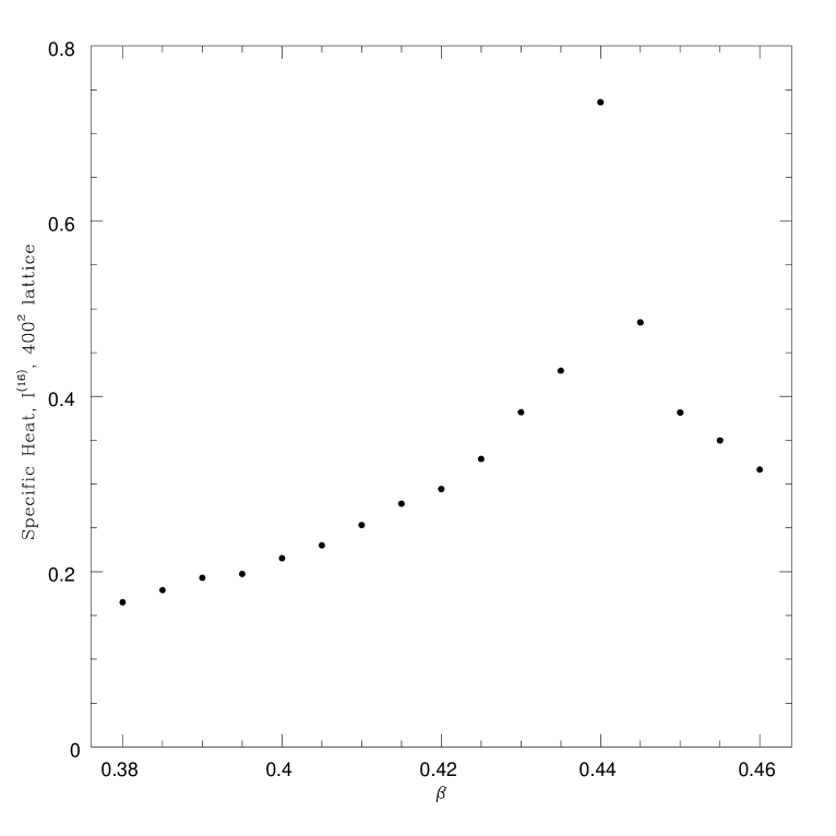
Figure 1: The specific heat (as computed from energy fluctuations), as a function of $\beta$ for the Ising model.

In fig. 1 we show the specific heat of the model. The point closer to criticality is the one at $\beta=.4400$ (as is fortunately obvious from the picture). Here, as well as in the following, the point size is of the order of magnitude of the statistical error, except for the point closer to criticality. The mild (logarithmic) divergence of the specific heat is at an inverse critical temperature which we can estimate from our data to be at $\beta_{c}=.440\pm.001$, in agreement with the known exact value.

In fig. 2 we show the correlation length $\xi\equiv\xi(5)$ (see (7)), which diverges at $T_{c}$ with a critical exponent $\nu=1$. We plot $\xi$ for $\xi\ll L$.

The second set of numerical simulations refer to model ${\cal I}^{(6)}$. We show respectively the specific heat and the correlation length in figs. 3 and 4.

These two figures strongly suggest that $T_{c}^{({\cal I}^{(6)})}<T_{c}^{({\cal I}^{(16)})}$: the critical temperature of the constrained model is smaller than the one of the original model. At the critical temperature of the Ising model the constrained model does not show a critical behavior. We estimate

$$\beta_{c}^{({\cal I}^{(6)})}=.4775\pm.0025\ .$$ (20)

The correlation length of model ${\cal I}^{(6)}$ is finite at the critical temperature of the Ising model; we estimate (see (8) for the definition and note that it is defined in units of the original lattice):

$$\xi_{(2)}\equiv\xi_{(2)}(5)\simeq 11.5\pm 0.5\ \quad,\quad\hbox{if }\beta=\beta_{c}^{({\cal I}^{(16)})}$$ (21)

This is in agreement with the numerical calculations related to the $DSU$ condition, that we shall discuss in the following section. In fact we find that the inequality (19) of section 4 is satisfied for $L>L_{c}$, with $L_{c}\simeq 5\xi$.

As we have already said, we have also simulated the model restricted to $4$ states (by forbidding turnons), which is equivalent to two decoupled Ising models. In figures 5 and 6 we show the specific heat and the correlation length; they clearly show criticality at $T_{c}^{({\cal I}^{(4)})}=T_{c}^{({\cal I}^{(16)})}$. Note that the correlation length is larger than in model ${\cal I}^{(16)}$, as one expects because the effective lattice spacing of the two independent Ising models is half the spacing in the original lattice. The ratio between the two correlations lengths should indeed be exactly $2$, if we could calculate the limit of $\xi_{(2)}(t)$ as $t\to\infty$.

In order to better characterize the nature of the transition for the constrained model ${\cal I}^{(6)}$ we will present some more data. As discussed in section 3, at $T=0$ the ${\cal I}^{(6)}$ model has $4$ ground states, with broken translational symmetry. We define $\rho_{i}$, $i=1,\ldots,4$ the projection of a given configuration over the $i-th$ ground state (we count the number of blocks which fit the ground state pattern, and we normalize with the total number of blocks). We define:

$$\rho\equiv\frac{1}{4}(\rho_{1}+\rho_{2}+\rho_{3}+\rho_{4})\ .$$ (22)

Let us remind again that the ground states do not include turnons. The turnon density is $(1-4\rho)$, and tends to zero for $\beta\to\infty$. In fig. 7 we plot $\rho$ as a function of $T$ for model ${\cal I}^{(6)}$. The density of turnons at $\beta=.4407$, the critical point of the full $2D$ Ising model, is close to $.06$, and is determining the finite correlation length.

Spontaneous symmetry breaking is signaled by the non-vanishing, in the infinite volume limit, of $\sigma$ defined by

$$\sigma\equiv\frac{1}{4}\sum_{i=1}^{4}(\rho_{i}-\rho)^{2}\ .$$ (23)

In the symmetric phase $\sigma\to 0$ in the infinite volume limit. In the broken phase the system aligns in one of the $4$ ground states (tunneling, at finite volume, among the different layered ground states), and $\sigma$ is non zero. We plot $\sigma$ in fig. 8. The location of the critical point is signaled with high precision from the drastic change in $\sigma$.

6 Numerical Results: the Dobrushin-Shlosman Condition

As discussed at the end of section 4 we have used the inequality (19) to obtain some reasonable insight about the validity of the Dobrushin-Shlosman uniqueness condition, which is too difficult to verify also numerically for volumes as large as needed in our case. However, even the task of checking numerically the inequality (19) is indeed a difficult one, with respect to the calculations of the previous section. In fact in this case one has to control the whole distribution. This is quite difficult, if compared with the simple task of computing averages of some observable quantities. The internal energy, for example, is peaked close to expectation value; hence, in order to compute its expectation value, one just needs to explore a very restricted part of the phase space. A computation of ${\cal M}_{L}$ (see (19)) demands, on the contrary, as we will see, a very large statistics.

In our simulations we have considered a sequence of cubes of side size $L$ and, after selecting $L$ and the number $I$ of Monte Carlo sweeps (we define a Monte Carlo sweep as the update of all lattice sites), we have chosen $N$ different random boundary condition, by assigning to the boundary sites the value $+$ or $-$ with equal probability. We shall call $\tau_{k}$, $k=1,\ldots,N$ these boundary conditions.

For each $\tau_{k}$ we have selected (randomly) a boundary couple of adjacent sites belonging to the same boundary block and we have considered the four boundary conditions $\tau_{k}^{j}$, $j=1,\ldots,4$, differing from each other only in the chosen boundary block, by changing in all possible ways the values of the two spins. We have done $4$ Monte Carlo runs with the four boundary conditions and, during these runs, we have recorded the number of times each block variable has visited each of the $6$ allowed states, by constructing

$$\tilde{N}_{\tau_{k}^{j}}(i,S_{i})\ ,$$ (24)

where $j$ ranges over the $4$ different values, $i$ ranges over the $(L/2)\times(L/2)$ blocks and $S_{i}$ ranges over the $6$ allowed block configurations. $\tilde{N}$ is normalized in such a way that

$$\sum_{S_{i}}\tilde{N}_{\tau_{k}^{j}}(i,S_{i})=1\ .$$ (25)

The quantity $\Delta_{L/2}$ of (19) was then calculated as

$$\Delta_{L/2}\equiv\max_{k=1,\ldots,N}\ \max_{j\not=l;j,l=1,\dots,4}\{\frac{1}{2}\sum_{i,S_{i}}|\tilde{N}_{\tau_{k}^{j}}(i,S_{i})-\tilde{N}_{\tau_{k}^{l}}(i,S_{i})|\}\ ,$$ (26)

In our simulations we have used $L=8$, $16$, $32$, $64$, $N$ of order $100$ and values of $I$ ranging from $4000$ to $4\ 10^{6}$ (for the largest value of $L$).

In fig. 9 we plot the quantity ${\cal M}_{L}$ of (19) as a function of the inverse square root of the run length, for different lattice sizes and number of iterations. The straight lines are our best linear fit, which turns out to be the right ansatz for the observed behavior.

The inequality (19) is satisfied only on the $64^{2}$ lattice, and it is violated on smaller lattices. Our best fits give

$${\cal M}_{8} = 2.10+\frac{17}{\sqrt{I}}\ ,$$

$${\cal M}_{16} = 1.83+\frac{83}{\sqrt{I}}\ ,$$ (27)

$${\cal M}_{32} = 1.32+\frac{229}{\sqrt{I}}\ ,$$

$${\cal M}_{64} = 0.58+\frac{706}{\sqrt{I}}\ .$$

There is indeed a big contribution due to the fact that we are adding a finite number of positive random numbers. Only in the limit of large number of iterations, $I\to\infty$, this contribution goes to zero. In order to minimize this effect we have also run simulations with the same boundary condition $\tau_{k}$, for each $k$. The average value of the difference

$$\{\frac{1}{2}\sum_{i,S_{i}}|\tilde{N}_{\tau_{k}}(i,S_{i})-\tilde{N^{\prime}}_{\tau_{k}}(i,S_{i})|\}$$

obtained in these conditions has been subtracted from ${\cal M}_{L}$ in order to define $\tilde{\cal M}_{L}$. The contribution we have subtracted from ${\cal M}_{L}$ goes to zero in the limit $I\to\infty$, making $\tilde{\cal M}_{L}$ a good estimator for the inequality (19). We plot $\tilde{\cal M}_{L}$ in fig. 10. Our best fits for $\tilde{\cal M}_{L}$ give

$$\tilde{\cal M}_{8} = 2.11-\frac{17}{\sqrt{I}}\ ,$$

$$\tilde{\cal M}_{16} = 1.83-\frac{4.0}{\sqrt{I}}\ ,$$ (28)

$$\tilde{\cal M}_{32} = 1.31+\frac{12.0}{\sqrt{I}}\ ,$$

$$\tilde{\cal M}_{64} = 0.60+\frac{205}{\sqrt{I}}\ .$$

The constant term coincides, as it should, with the one we get for $\cal M$, with very good precision. On the contrary slopes are smaller, indicating that $\tilde{\cal M}$ is, as expected, a better estimator than $\cal M$ when using a finite number of iterations.

7 Conclusions

From the numerical results on specific heat and correlation length, which are based on “traditional” numerical methods to detect a (second order) phase transition, we can be reasonably sure that, indeed, the critical temperature of ${\cal I}^{(6)}$ model is strictly less than $T_{c}^{Ising}$. The remark on the isomorphism between ${\cal I}^{(4)}$ and the full Ising model ${\cal I}^{(16)}$ shows that one cannot, a priori, expect any monotonicity property of critical temperatures in terms of imposed constraints. Our numerical results indicate that, by imposing the constraint $m_{i}=0$, $\forall\;B_{i}$, one decreases the critical temperature whereas, by enhancing again the constraint via the further elimination of the turnons, one increases the critical temperature since it goes back to $T_{c}^{Ising}$.

To theoretically analyze this apparently strange behavior it seems useful to use some generalized form of Fortuin-Kasteleyn representation of the Ising model sufficiently “elastic” to include, in the same set-up of random-cluster models, the three models ${\cal I}^{(16)}$, ${\cal I}^{(6)}$, ${\cal I}^{(4)}$ that we have considered ([10]).

On the other hand to rigorously implement the Cassandro-Gallavotti program one needs a strong notion of absence of phase transition, namely to verify some strong mixing condition SM.

We say that a Gibbs measure $\mu_{\Lambda}^{\tau}$ in $\Lambda$ with $\tau$ boundary conditions outside $\Lambda$ satisfies a strong mixing condition $SM(\Lambda,C,\gamma)$ if the influence at $x\;\in\;\Lambda$ of a local change in $y\;\in\;\Lambda^{c}$ of the value of the conditioning spin configuration $\tau$ decays as

$$Ce^{-\gamma|x-y|}$$

Of course $SM(\Lambda,C,\gamma)$ implies $WM(\Lambda,C,\gamma)$ (see section 4); moreover $SM$ $(\Lambda,$ $C,$ $\gamma)$ is interesting when it is valid for a class of volumes $\Lambda$ invading ${\bf Z^{d}}$ with $C$ and $\gamma$ independent of $\Lambda$.

As we have said in section 2, in [20] it is proven that, in two dimensions, $WM$ implies $SM$ at least for sufficiently regular regions $\Lambda$. $SM$ would be certainly largely sufficient to compute, via the Cassandro-Gallavotti method, the renormalized potentials whereas, in general, $WM$ alone will not.

In section 6 we have analyzed a sort of lower bound (involving variation distance) for the quantity appearing in the Dobrushin-Shlosman uniqueness condition (implying $WM$ and so, since we are in $2D$, $SM$). This is only an (almost) necessary condition to be verified in order to satisfy the true condition $DSU$. It only gives an indication in the sense of the possibility to verify $DSU$ (which involves Vasserstein distance).

It is clear that one needs to consider squared regions containing about $30$ $\times$ $30$ blocks. This rules out, at least with the present time computers, the possibility of a computer-assisted proof. Then it would be important to be able to find a “Montecarlo” method to “measure” the quantity (Vasserstein distance) appearing in $DSU$.

It would also be interesting, in general, to find an algorithm, easily implementable in a computer, to evaluate the Vasserstein distance between two Gibbs measures with different boundary conditions. This will be the object of further investigations.

Figure 2: The correlation length $\xi$ as a function of $\beta$, for the Ising model.

Figure 3: As in fig. 1, but for the $6$ block state constrained Ising model, ${\cal I}^{(6)}$.

Figure 4: As in fig. 2, but for the $6$ block state constrained Ising model, ${\cal I}^{(6)}$.

Figure 5: As in fig. 1, but for the $4$ block state constrained Ising model, ${\cal I}^{(4)}$.

Figure 6: As in fig. 2, but for the $4$ block state constrained Ising model, ${\cal I}^{(4)}$.

Figure 7: $\rho$ as a function of $\beta$ for the $6$ block state model ${\cal I}^{(6)}$.

Figure 8: $\sigma$ as a function of $\beta$ for the $6$ block state model ${\cal I}^{(6)}$.

Figure 9: ${\cal M}_{L}$ as a function of the inverse square root of the number of sweeps, for different lattice sizes. Straight lines are best linear fits. Empty triangles for $L=8$, filled triangles for $L=16$, crosses for $L=32$ and filled dots for $L=64$.

Figure 10: As in fig. 9, but for $\tilde{\cal M}_{L}$.

References

- [1] C. Cammarota, The Large Block Spin Interaction, Il Nuovo Cimento 96B (1986) 1-16.
- [2] M. Cassandro and G. Gallavotti, The Lavoisier Law and the Critical Point, Il Nuovo Cimento 25B (1975) 691.
- [3] R. L. Dobrushin, Prescribing a System of Random Variables by Conditional Distributions, Theory of Prob. Appl. 15 (1970) 453-486.
- [4] R. L. Dobrushin and S. Shlosman, Constructive Criterion for the Uniqueness of Gibbs Fields, Stat. Phys. and Dyn. Syst., Birkhauser (1985) 347-370.
- [5] R. L. Dobrushin and S. Shlosman, Completely Analytical Gibbs Fields, Stat. Phys. and Dyn. Syst., Birkhauser (1985) 371-403.
- [6] R. L. Dobrushin and S. Shlosman, Completely Analytical Interactions Constructive Description, Journ. Stat. Phys. 46 (1987) 983-1014.
- [7] A. C. D. van Enter, R. Fernández and A. D. Sokal, Regularity Properties and Pathologies of Position-Space Renormalization-Group Transformations: Scope and Limitations of Gibbsian Theory, Journ. Stat. Phys. 72 (1994) 879-1167.
- [8] R. Fernandez and C. Pfister, Non Quasi-Local Projections of Gibbs States, preprint (1994).
- [9] R. B. Griffiths and P. A. Pearce, Mathematical Properties of Position-Space Renormalization Group Transformations, Journ. Stat. Phys. 20 (1979) 499-545.
- [10] J. Grimmett, private communication.
- [11] D. W. Heermann and A. N. Burkitt, Physica A162 (1990) 409.
- [12] R. B. Israel, Banach Algebras and Kadanoff Transformations, in Random Fields, J. Fritz, J. L. Lebowitz and D. Szasz editors (Esztergom 1979), Vol. II, 593-608 (North-Holland, Amsterdam 1981).
- [13] T. Kennedy, Some Rigorous Results on Majority Rule Renormalization Group Transformations near the Critical Point, preprint.
- [14] O.K. Kozlov, Gibbs Description of a System of Random Variables, Probl. Inform. Transmission. 10 (1974) 258-265.
- [15] J. Lorinczi and K. Vande Velde, A Note on the Projection of Gibbs Measures, preprint (1994).
- [16] F. Martinelli and E. Olivieri, Finite Volume Mixing Conditions for Lattice Spin Systems and Exponential Approach to Equilibrium of Glauber Dynamics, Proceedings of 1992 Les Houches Conference on Cellular Automata and Cooperative Systems, N. Boccara, E. Goles, S. Martinez and P. Picco editors (Kluwer 1993).
- [17] F. Martinelli and E. Olivieri, Approach to Equilibrium of Glauber Dynamics in the One Phase Region I. The Attractive Case, in press on Commun. Math. Phys. (1994).
- [18] F. Martinelli and E. Olivieri, Approach to Equilibrium of Glauber Dynamics in the One Phase Region II. The General Case, in press on Commun. Math. Phys. (1994).
- [19] F. Martinelli and E. Olivieri, Some Remarks on Pathologies of Renormalization Group Transformations for the Ising model, Journ. Stat. Phys. 72 (1994) 1169-1177.
- [20] F. Martinelli, E. Olivieri and R. Schonmann, For Lattice Spin Systems Weak Mixing Implies Strong Mixing, in press on Commun. Math. Phys. (1994).
- [21] E. Olivieri, On a Cluster Expansion for Lattice Spin Systems: a Finite Size Condition for the Convergence, Journ. Stat. Phys. 50 (1988) 1179-1200.
- [22] E. Olivieri and P. Picco, Cluster Expansion for -Dimensional Lattice Systems and Finite Volume Factorization Properties, Journ. Stat. Phys. 59 (1990) 221-256.
- [23] R. H. Schonmann, Projections of Gibbs Measures May Be Non-Gibbsian, Commun. Math. Phys. 124 (1989) 1-7.