Crossover Driven by Time-reversal Symmetry Breaking in Quantum Chaos

Abstract

Parametric correlations of energy spectra of quantum chaotic systems are presented in the orthogonal-unitary and symplectic-unitary crossover region. The spectra are allowed to disperse as a function of two external perturbations: one of which preserves time-reversal symmetry, while the other violates it. Exact analytical expressions for the parametric two-point autocorrelation function of the density of states are derived in the crossover region by means of the supermatrix method. For the orthogonal-unitary crossover, the velocity distributions is determined and shown to deviate from Gaussian.

Spectral properties of quantum chaotic systems are well described by the Wigner-Dyson statistics of random matrix theory [3]. Originally introduced to study complex nuclei, random matrix theory (RMT) was found to be relevant to the spectral statistics of disordered metallic particles (quantum dots) [4, 5, 6], as well as quantum chaotic systems in general (e.g., chaotic billiards) [7]. The most striking feature is universality: when energies scaled by the mean level spacing, their distribution depends only on the symmetry of the Hamiltonian, irrespective of microscopic details. Typically systems belong to one of three universality classes: orthogonal (spinless) and symplectic (with spin-orbit interaction) for those which are invariant under time-reversal invariant systems, and unitary for those which are not. Starting from the Schrödinger equation with a random potential, Efetov has developed a field theoretic description of disordered metals, based on a supermatrix nonlinear $\sigma$-model [5]. He demonstrated that, up to the Thouless energy, the density of states correlators for the three universality classes are identical to those derived from RMT.

Subsequently Pandey and Mehta extended RMT to examine crossover behavior where the symmetry of the system gradually changes from one pure symmetry to another [8]. They obtained an analytical expression for the density of states correlator, i.e., the two-point cluster function, and related quantities. (A result recently rederived recently by the supermatrix method [9].) The resulting description of the orthogonal-unitary crossover was numerically justified for a disordered metallic ring with Aharonov-Bohm flux [10].

A second approach to quantum chaos is to examine correlations of a Hamiltonian $H(X)$ which depend on an external parameter $X$. Beginning with the work of Pechukas[11] and Yukawa [12], problems of this kind have attracted great interest most recently [13, 14]. By making use of an appropriate rescaling, parametric correlations of the density of states as well as response functions were also shown to be universal [15, 16].

In this Letter, we will examine the universal parametric correlations in the orthogonal-unitary crossover region. For completeness, we mention (but do not discuss) the result for symplectic-unitary crossover. We are motivated by problems where the Hamiltonian $H(X_{o},X_{u})$ depends on two external parameters $X_{o}$ and $X_{u}$, where the former preserves the time-reversal symmetry whereas the second violates it. Although the spectral statistics of $H(X_{o},X_{u}=0)$ belong to the orthogonal ensemble, gradually driven to unitary by introducing T-invariance breaking parameter, $X_{u}$.

Parametric correlations in the orthogonal-unitary crossover are relevant to many problems. In a recent experiment [17], the correlator of differential conductance was measured as a function of magnetic field, $X_{u}$, in a heavily doped quantum dot. These measurements were directly related to density correlators in the crossover region, considered below. At the same time, one can imagine gate voltage serving as second parameter $X_{o}$, which perturbs the system but conserves T-invariance. A second example could involve an irregular ballistic cavity, or billiard in which a potential, $X_{o}$, changes the shapes of the boundary, while a magnetic field acts as a T-breaking perturbation.

Our aim here is to determine the parametric autocorrelator of density of states

$$K(\Omega,X_{o},X_{u};\bar{X})=\left\langle{\nu(E,\bar{X}_{o}-{\textstyle{{X_{o}}\over 2}},\bar{X}-{\textstyle{{X_{u}}\over 2}})\,\nu(E+\Omega,\bar{X}_{o}+{\textstyle{{X_{o}}\over 2}},\bar{X}+{\textstyle{{X_{u}}\over 2}})}\right\rangle,$$ (1)

where $\nu(E,X_{o},X_{u})=\sum_{n}{\delta(E-E_{n}(X_{o},X_{u}))}$ is the density of states and $E_{n}(X_{o},X_{u})$ are eigenenergies of the Hamiltonian $H(X_{o},X_{u})$. The statistical average denoted by $\langle\cdots\rangle$ can be performed over certain interval of the energy and/or external parameters. $K$ depends on the average of the unitary parameter $\bar{X}$, as well as on differences of parameters $X_{o,u}$ and energies, $\Omega$. $\bar{X}$ serves as a crossover parameter from orthogonal to unitary symmetry.

Following Ref. [15, 16], we switch from $\{\Omega,X_{o},X_{u},\bar{X}\}$ to dimensionless variables $\{\omega,x_{o},x_{u},\bar{x}\}$ (conventionally written as lower case),

$$\omega=\Omega/\Delta;\quad\varepsilon_{n}=E_{n}/\Delta$$ (2)

$$x_{o}=\sqrt{C_{o}(0;\bar{X}=0)}\,X_{o};\quad x_{u}=\sqrt{C_{u}(0;\bar{X}\rightarrow\infty)}\,X_{u};\quad\bar{x}=\sqrt{C_{u}(0;\bar{X}\rightarrow\infty)}\,\bar{X},$$ (3)

$$C_{o,u}(0,\bar{X})=\left\langle{\left({{{\partial\varepsilon_{n}(X_{o},X_{u})}\over\partial X_{o,u}}}\right)^{2}}\right\rangle,$$ (4)

where $\Delta=\langle\nu\rangle^{-1}$ is the mean level spacing of the spectrum. We note that rescaling for $X_{o}$ is defined in the orthogonal limit, and for $X_{u}$ and $\bar{X}$ at the unitary limit, which follows the conventions of both. We show that a dimensionless correlator defined by

$$k(\omega,x_{o},x_{u};\bar{x})=\Delta^{2}K(\Omega,X_{o},X_{u};\bar{X})-1,$$ (5)

is a universal function of all dimensionless variables $\omega$, $x_{o,u}$, and $\bar{x}$.

Consider the $N\times N$ random matrix $H(X_{o},X_{u})=H_{0}+X_{o}H_{s}+X_{u}H_{a}$, where $H_{0}$ and $H_{s}$ are real symmetric matrices and $H_{a}$ is an antihermitian matrix [8], the transition from orthogonal to unitary symmetry for $K(\Omega,X_{o},X_{u};\bar{X})$ occurs at $\bar{X}$ of the order of $1/\sqrt{N}$ or equivalently $\bar{x}\sim 1$. Thus all non-universal effects such as $\bar{X}$-dependence of $\Delta$ are negligible in the limit $N\rightarrow\infty$. As a result, crossover behavior of $k(\omega,x_{o},x_{u};\bar{x})$ is universal.

To evaluate the $k(\omega,x_{o},x_{u};\bar{x})$, we use the zero dimensional supermatrix nonlinear $\sigma$-model, which can be derived from the disordered metallic grain with large dimensionless conductance. This model serves as an underlying universal model for describing spectral statistics of quantum chaotic systems [15, 16] even in the orthogonal-unitary crossover region [9]. Following the notation of Ref. [5], $k(\omega,x_{o},x_{u};\bar{x})$ can be expressed through the nonlinear $\sigma$-model as

$$k(\omega,x_{u},x_{o};\bar{x})=-\mbox{Re}\,\int{\cal D}Q\,e^{-F[Q]}{(Q-\Lambda)_{33}^{11}(Q-\Lambda)_{33}^{22}},$$ (6)

$$F[Q]={{i\pi\omega}\over 4}\mbox{STr}\left({\Lambda Q}\right)-{{\pi^{2}}\over 8}\mbox{STr}\left[{Q,\bar{x}\tau_{3}+{{x_{u}}\over 2}\tau_{3}\Lambda}\right]^{2}-{{\pi^{2}x_{o}^{2}}\over{64}}\mbox{STr}\left[{\Lambda,Q}\right]^{2},$$ (7)

where $Q$ is a supermatrix. The extension to parametric correlation functions is straightforwardly done [18]. Performing the definite integral over the supermatrix, we obtain for orthogonal-unitary crossover:

$$k_{ou}(\omega,x_{o},x_{u};\bar{x})=\mbox{Re}\int_{-1}^{1}\!d\lambda\int_{1}^{\infty}\!d\lambda_{1}\int_{1}^{\infty}\!d\lambda_{2}\;e^{-F}\;W_{+}(\omega,x_{o},x_{u};\bar{x}),$$ (8)

where

$$F= -i\pi\omega|\lambda_{1}\lambda_{2}-\lambda|+\pi^{2}\bar{x}^{2}|2\lambda_{2}^{2}-\lambda^{2}-1|+{{\pi^{2}x_{u}^{2}}\over 4}|2\lambda_{1}^{2}-\lambda^{2}-1|$$ (10)

$$+{\pi^{2}x_{o}^{2}\over 4}|2\lambda_{1}^{2}\lambda_{2}^{2}-\lambda^{2}-\lambda_{1}^{2}-\lambda_{2}^{2}+1|,$$

$$W_{\pm}(\omega,x_{o},x_{u};\bar{x})={(\lambda_{1}\lambda_{2}-\lambda)^{2}\over(\lambda_{1}^{2}+\lambda_{2}^{2}+\lambda^{2}-2\lambda\lambda_{1}\lambda_{2}-1)}\left[\pm{(1-\lambda^{2})\cosh\alpha-(\lambda_{1}^{2}-\lambda_{2}^{2})\sinh\alpha\over(\lambda_{1}^{2}+\lambda_{2}^{2}+\lambda^{2}-2\lambda\lambda_{1}\lambda_{2}-1)}\right.$$ (11)

$$\qquad\left.+\pi^{2}\left[(4\bar{x}^{2}\lambda_{2}^{2}-x_{u}^{2}\lambda_{1}^{2})\sinh\alpha+(2\bar{x}^{2}e^{-\alpha}+{x_{u}^{2}\over 2}e^{\alpha})(1-\lambda^{2})\right]\right\},$$ (12)

and we define $\alpha=\pi^{2}(\bar{x}^{2}-x_{u}^{2}/4)|1-\lambda^{2}|$. For completeness, we include the analogous expression for symplectic-unitary crossover:

$$k_{su}(\omega,x_{o},x_{u};\bar{x})=\mbox{Re}\int_{1}^{\infty}\!d\lambda\int_{-1}^{1}\!d\lambda_{1}\int_{0}^{1}\!d\lambda_{2}\;e^{-F}\;W_{-}(\omega,x_{o},x_{u};\bar{x}),$$ (13)

where $x_{o}$ plays a role as any T-invariance perturbation parameter in this case. Hereafter we restrict ourselves to the orthogonal-unitary crossover case for brevity.

We first check various limiting behaviors of Eq. (8). The orthogonal limit straightforwardly gives the same result of Ref. [15] when we set $\bar{x},x_{u}\to 0$. In the unitary limit ($\bar{x}\rightarrow\infty$, and $x_{o}\rightarrow 0$), we can recognize the leading contribution coming from the term proportional to $\bar{x}^{2}\exp\left({-F+\alpha}\right)$. After $\lambda_{2}$ integration, the expression is reduced to the same expression for the pure unitary case in Ref. [15]. Another interesting limit is the large $\omega$ asymptotics, which can be obtained by expanding the integrand of Eq. (8) around $\lambda=\lambda_{1}=\lambda_{2}=1$, and replacing the integral region over $\lambda$ by $(-\infty,1)$. After straightforward but lengthy calculation, we can show that the large $\omega$-asymptotics acquires the diffusive form, which can be interpreted as the Diffuson and Cooperon modes in disordered systems:

$$k(\omega,x_{u},x_{o};\bar{x})\cong{1\over 2\pi^{2}}\mbox{Re}\left[\left({-i\omega+\pi x_{o}^{2}/2+\pi x_{u}^{2}}\right)^{-2}+\left({-i\omega+\pi x_{o}^{2}/2+4\pi\bar{x}^{2}}\right)^{-2}\right].$$ (14)

We can use $k(\omega,x_{u},x_{o};\bar{x})$ to obtain the velocity (i.e., single level current $\partial\varepsilon_{n}/\partial x_{o,u}$) distribution functions. Here we can define the two kinds of rescaled velocities both in the orthogonal and unitary directions by ${\partial\varepsilon_{n}}/{\partial x_{o,u}}$. Their probability distribution can be obtained from the formula $f_{o,u}(v;\bar{x})\equiv\left\langle{\delta\left(v-\partial\varepsilon_{n}/\partial x_{o,u}\right)}\right\rangle=\lim_{x_{o},x_{u}\to 0}x_{o,u}\,k(\omega=vx_{o,u},\>x_{o},x_{u};\bar{x})$ [19]. Substituting our exact result Eq. (8), we obtain

$$f_{o}(v,\bar{x})={1\over\sqrt{2\pi}}\int_{0}^{\infty}{dt\,\left[{1+{{1-A(\bar{x})}\over{2\pi^{2}\bar{x}^{2}}}\left({t-1}\right)}\right]\,\sqrt{{{t+2\pi^{2}\bar{x}^{2}}\over{t+\pi^{2}\bar{x}^{2}}}}\;\exp\left[{-t-{{v^{2}}\over 2}\left({{{t+2\pi^{2}\bar{x}^{2}}\over{t+\pi^{2}\bar{x}^{2}}}}\right)}\right]},$$ (16)

$$f_{u}(v,\bar{x})={e^{-v^{2}/2}\over\sqrt{2\pi}}\left[{1-A(\bar{x})+2\pi^{2}\bar{x}^{2}A(\bar{x})\int^{\infty}_{1}{dt\sqrt{t}\;e^{(v^{2}/2+2\pi^{2}\bar{x}^{2})(1-t)}}}\right],$$ (17)

where $A(\bar{x})\equiv e^{-2\pi^{2}\bar{x}^{2}}\int_{0}^{1}{e^{2\pi^{2}\bar{x}^{2}\lambda^{2}}\,d\lambda}$. The function $A(\bar{x})$ behaves like $1-4\pi^{2}\bar{x}^{2}/3$ for small $\bar{x}$, but vanishes exponentially for large $\bar{x}$. Their limiting behaviors are easy to understand. In the unitary limit ($\bar{x}\to\infty$), the velocity distribution has a Gaussian in both directions,

$$f_{o}(v;\bar{x}\to\infty)={\exp\left[{-v^{2}}\right]\over\sqrt{\pi}}\>;\quad f_{u}(v;\bar{x}\to\infty)={\exp\left[{-v^{2}/2}\right]\over\sqrt{2\pi}}.$$ (18)

This means that there is no qualitative difference between the unitary and the orthogonal perturbations, since T-invariance is already fully broken in the unitary limit. On the other hand, in the orthogonal limit, the two velocity distributions behave quite differently.

$$f_{o}(v;\bar{x}\to 0)={{\exp\left[{-v^{2}/2}\right]}\over\sqrt{2\pi}}\>;\quad f_{u}(v;\bar{x}\to 0)=\delta(v).$$ (19)

$f_{u}(v;\bar{x}\to 0)$ collapses to a $\delta$-function, since $\varepsilon(x_{o},x_{u})-\varepsilon(x_{o},0)\propto x_{u}^{2}$ for $x_{u}\rightarrow 0$. However there is nothing special in the orthogonal direction, so that its distribution is again Gaussian with twice as wide variance as the unitary limit. The velocity distribution interpolates smoothly between these two limiting cases.

Since the average velocities vanish, the velocity distributions in the crossover region can be characterized by their variances: $c_{o,u}(0;\bar{x})\equiv\left\langle(\partial\varepsilon_{n}/\partial x_{o,u})^{2}\right\rangle$. According to Eq. (11), they are

$$c_{o}(0;\bar{x}) ={{1+A(\bar{x})}\over 2}+{{(2\pi^{2}\bar{x}^{2}+1)A(\bar{x})-1}\over 2}\mbox{Ei}(-2\pi^{2}\bar{x}^{2})\exp(2\pi^{2}\bar{x}^{2}),$$ (21)

$$c_{u}(0;\bar{x}) =1-\left[{1+2\pi^{2}\bar{x}^{2}\exp(2\pi^{2}\bar{x}^{2})\,\mbox{Ei}(-2\pi^{2}\bar{x}^{2})}\right]\,A(\bar{x}),$$ (22)

where $\mbox{Ei}(-z)=\int^{\infty}_{z}dte^{-t}/t$ is the exponential integral function. Hence in the limiting case for $\bar{x}\ll 1$, we find

$$c_{o}(0;\bar{x}\to+0) \cong 1+{{\pi^{2}\bar{x}^{2}}\over 3}\ln(2\pi^{2}\bar{x}^{2}),$$ (24)

$$c_{u}(0;\bar{x}\to+0) \cong-2\pi^{2}\bar{x}^{2}\ln(2\pi^{2}\bar{x}^{2}).$$ (25)

These logarithmic dependencies can be understood by a $2\times 2$ random matrix model [20], since the nearest neighboring pairs of energy levels make the dominant contribution for small $\bar{x}$. Around the orthogonal limit, eigenenergies can be considered as $\varepsilon(\bar{x})\approx\sqrt{\varepsilon^{2}(0)+\bar{x}^{2}}$, where $\varepsilon$ is assumed to obey the Gaussian orthogonal ensemble. Therefore $c_{u}(0;\bar{x})$ can be evaluated as

$$c_{u}(0;\bar{x})\approx\int_{0}^{\infty}{d\varepsilon\,\left({\partial\varepsilon/\partial\bar{x}}\right)^{2}P_{\rm GOE}(\varepsilon)}\approx\int_{\bar{x}}{d\varepsilon\,\bar{x}^{2}/\varepsilon}\approx-\bar{x}^{2}\ln(\bar{x}).$$ (26)

This demonstrates that the logarithmic dependence is specific to the orthogonal-unitary crossover. By contrast, $c_{u}(0;\bar{x})\approx\bar{x}^{5}$ in the symplectic-unitary crossover because $P_{\rm GSE}(\varepsilon)\sim\varepsilon^{4}$ for small $\varepsilon$.

In Fig. 1, we compare our analytical results of $c_{o,u}$ with numerical results, obtained from the random matrix $H=H_{0}+X_{o}H_{s}+X_{u}H_{a}$, where $H_{0}$, $H_{s}$ and $H_{a}$ were defined previously. $\left\langle{(\partial E_{n}/\partial X_{o,u})^{2}}\right\rangle$ was determined numerically and rescaled according to Eqs. (2–4). As is seen in Fig. 1, agreement with Eqs. (21,b) is good, particularly for small $\bar{x}$.

So far, we have used the rescaled parameters which are determined in the unitary or orthogonal limit. However, in experimental situations, only the results in the crossover region may be obtained. For such a case, we propose here the local normalization scheme. While $\bar{x}$ and $x_{u}$ are formerly defined by Eqs. (3), what is actually observed at a fixed $\bar{X}$ is

$$\bar{y}^{2}=\left\langle{\left({{{\partial\varepsilon_{n}}\over{\partial X_{u}}}}\right)^{2}}\right\rangle_{\bar{X}}\bar{X}^{2};\quad\quad y_{o,u}^{2}=\left\langle{\left({{{\partial\varepsilon_{n}}\over{\partial X_{o,u}}}}\right)^{2}}\right\rangle_{\bar{X}}X_{o,u}^{2}.$$ (27)

To express all universal properties in terms of $\bar{y}$ and $y_{u}$ instead of $\bar{x}$ and $x_{u}$, we can make use of the relation between $\bar{y}$ and $\bar{x}$ ($y_{o,u}$ and $x_{o,u}$) and write

$$\bar{x}^{2}c_{u}(\bar{x})=\bar{y}^{2};\quad\quad x_{o,u}^{2}c_{o,u}(\bar{x})=y_{o,u}^{2}.$$ (28)

By calculating the function $\bar{x}=f(\bar{y})$ and $x_{o,u}=y_{o,u}/c_{o,u}(f(\bar{y}))$, we can express the universal dependence in terms of $\{y_{o},y_{u},\bar{y}\}$ rather than $\{x_{o},x_{u},\bar{x}\}$, which enables us to rescale the external parameters through a local point in the crossover region.

In conclusion, we have presented an analytical expression for the universal parametric correlations of density of states both in the orthogonal-unitary and symplectic-unitary crossover region of quantum chaotic systems. For the former, the velocity distribution functions both in the unitary and the orthogonal direction were presented analytically. In particular, the velocity distribution in the unitary direction shows continuous transition between a Gaussian and a $\delta$-function. Their variances both in the orthogonal and unitary directions are shown to have the logarithmic dependence around the orthogonal limit. In addition, we have also proposed a local rescaling scheme of data in the crossover region.

The authors are grateful to A. Altland, A. Andreev, K. B. Efetov, C. Itzykson, S. Iida, V. N. Prigodin, and U. Sivan for helpful and stimulating discussions. The work was supported by NSF Grant No. DMR 92-04480. N.T. also acknowledges the research fellowship from Murata Overseas Scholarship Foundation.

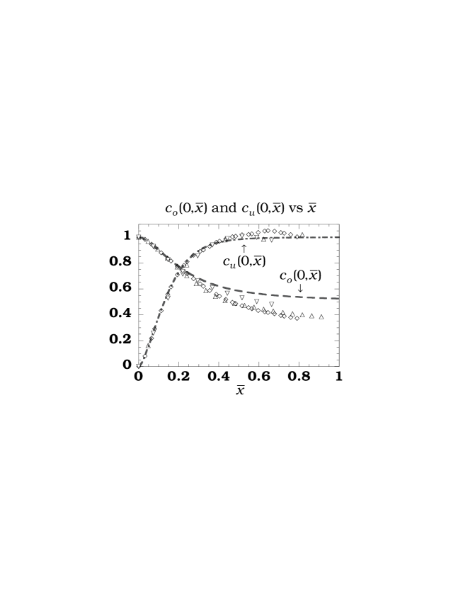
FIG. 1.: Comparison between numerical and analytical calculations of $c_{o,u}(0;\bar{x})$. Numerical calculations of $c_{o,u}$ were obtained from $25\times 25(\Diamond)$, $50\times 50(\bigtriangleup)$ and $100\times 100(\bigtriangledown)$ random matrices $H(X_{o},X_{u})=H_{0}+X_{o}H_{s}+X_{u}H_{a}$ described in the text. The dot-dashed and the dashed lines are analytical results for $c_{u}(0;\bar{x})$ and $c_{o}(0;\bar{x})$ given by Eqs. (21,b).

REFERENCES

[1]
On leave from Department of Applied Physics, University of Tokyo, Tokyo
113, Japan.
[2]
Present address: Department of Physics, Princeton University, Princeton,
New Jersey 08544.
[3]
For reviews, see M. L. Mehta, ‘Random Matrices — Revised and
Enlarged Second Edition’ (Academic Press Inc., San Diego, CA, 1991);
F. Haake, Quantum Signatures of Chaos (Springer-Verlag, Berlin,
1991).
[4]
L. P. Gor’kov and G. M. Eliashberg, Sov. Phys. JETP 21, 940
(1965).
[5]
K. B. Efetov, Adv. Phys. 32, 53 (1983).
[6]
B. L. Al’tshuler and B. I. Shklovskii, Sov. Phys. JETP 64, 127
(1986).
[7]
For a review, see O. Bohigas, in Chaos and Quantum Physics, edited
by M.-J. Giannoni, A. Voros, and J. Zinn-Justin (North-Holland,
Amsterdam, 1991).
[8]
A. Pandey and M. L. Mehta, Commun. Math. Phys. 16, 2655 (1983);
M. L. Mehta and A. Pandey, J. Phys. A 16 2655 and L601 (1983).
See also, J. B. French, V. K. B. Kota, A. Pandey, and S. Tomosovic, Ann.
Phys. 181, 198 (1988).
[9]
A. Altland, S. Iida, and K. B. Efetov, J. Phys. A 26, 3545 (1993).
[10]
N. Dupuis and G. Montambaux, Phys. Rev. B 43, 14390 (1991).
[11]
P. Pechukas, Phys. Rev. Lett., 51, 943 (1983).
[12]
T. Yukawa, Phys. Rev. Lett., 54, 1883 (1985).
[13]
M. Wilkinson, J. Phys. A 21, 4021 (1988); 22, 2795 (1989).
[14]
P. Gaspard, S. A. Rice, M. J. Mikeska, and N. Nakamura, Phys. Rev. A
42, 4015 (1990); D. Saher, F. Haake, and D. Gaspard, Phys. Rev. A
44, 7841 (1991); J. Zakrzewski and D. Delande, Phys. Rev. E 47, 1650 (1993).
[15]
B. D. Simons and B. L. Altshuler, Phys. Rev. Lett. 70, 4063
(1993); B. D. Simons and B. L. Altshuler, Phys. Rev. B 48, 5422
(1993); B. D. Simons, P. A. Lee, and B. L. Altshuler, Phys. Rev. B 48, 11450 (1993).
[16]
N. Taniguchi and B. L. Altshuler, Phys. Rev. Lett. 71, 4031
(1993); submitted to Phys. Rev. Lett. (unpublished).
[17]
U. Sivan et al., to be published in Europhys. Lett., Apr. 1994.
[18]
Although the parametric extension is straightforward in the supermatrix
method, the actual complexity of the analytical calculation will highly
depend on how the saddle-point manifold is parametrized. The
parametrization used for deriving our main result Eq.(8) is
the original one introduced in Ref. [5] and slightly
modified according to suggestions in the appendix of [21].
We remark that parametrization introduced in Ref. [9] leads
to a more cumbersome representation of Eq.(8).
[19]
V. E. Kravtsov and M. R. Zirnbauer, Phys. Rev. B 46, 4332 (1992).
[20]
A. Kamenev and D. Braun, (unpublished).
[21]
A. Altland, S. Iida, A. Müller-Groeling, and H. A. Weidenmüller,
Ann. Phys. 219, 148 (1992).
FIG. 1.:
Comparison between numerical and analytical calculations of
. Numerical calculations of were obtained
from , and
random matrices described in the text. The dot-dashed and the dashed lines
are analytical results for and given by
Eqs. (21,b).