On the $3d$ Ising Spin Glass

Abstract

We study the $3d$ Ising spin glass with $\pm 1$ couplings. We introduce a modified local action. We use finite size scaling techniques and very large lattice simulations. We find that our data are compatible both with a finite $T$ transition and with a $T=0$ singularity of an unusual type.

SCCS 532
Roma Tor Vergata ROM2F/93/94
Roma La Sapienza 967-93
cond-mat/9310041

1 Introduction

Three dimensional spin glasses [1] are a fascinating subject. Numerical simulations are here particularly interesting [2, 3, 4, 5, 6, 7], since for such model (the real thing) it is very difficult to obtain reliable analytical results. Up to date numerical simulations for the Ising case have shown a phenomenology very similar to the experiments on real spin glasses (for recent simulations and analytical results about, for example, aging phenomena, see [8]). The study of small size systems (up to a linear size $L=14$) has shown a reasonable agreement with the predictions of broken replica theory, but it is obscure how much information about the thermodynamic limit can be inferred from the behavior of small systems. In particular one has to be careful about extrapolating the pattern of replica symmetry breaking from small to large lattices. Here our aim has been to reconsider the whole subject and try to clarify the emerging physical picture at low temperature $T$.

We will deal with the problem of the nature and the existence of a phase transition. A cursory look at the history of the subject is useful. If we look at the period that begins when people investigated first the subject of disordered spin systems we can easily establish that there have been periodic oscillations, with periods of the order of $7$ years. Researchers in the field have been oscillating between the credence that there is a sharp transition and the belief that there are no transitions at all (as is maybe true in real glasses) and that when lowering $T$ there is only a gradual freezing of the dynamical degrees of freedom. At the beginning theoreticians had (at equal time) a different credence from the experimental researchers. The two groups had a different frequency of oscillations, and now there is consensus that the system undergoes some kind of phase transition.

We have run long numerical simulations at various temperatures, doing our best to distinguish among these two possibilities. In our analysis we have been very much inspired by the approach and the doubts of Bhatt, Morgenstern, Ogielsky and Young [2, 3, 4, 5, 6, 7], and over their results we have tried to build and improve. We have found that the whole set of our data is well compatible with the possibility that there is a transition at a given non-zero $T$. Such a transition would be characterized by a large value of the exponent $\gamma$, close to $2.5$ ($\gamma$ is the usual susceptibility exponent, which will be defined later in a more precise way). The whole set of data is also compatible with a large set of possible reasonable functional dependencies, which imply a transition temperature of zero. Recent studies using improved Monte Carlo techniques [9, 10, 11] also find that doubts about the existence of a finite $T$ critical behavior are justified [12]. The difficulty of resolving among the two behaviors is because a large value of $\gamma$ implies that the system is not far from being at its lower critical dimension (at which, according to the conventional wisdom, $\gamma\to\infty$). The distinction among a system at the critical dimension and a system very close to it is particularly difficult to pin. We believe however that we are not too far from being able to resolve among the two models and that an increase in the simulation time of one or two orders of magnitude can clarify the situation. Of course precise theoretical predictions on the behavior of spin glasses at the lower critical dimensions would be invaluable.

We have been studying the $3d$ Ising spin glass, with $\pm 1$ couplings, but we have not used the standard first neighbor model. Hoping for some gain we have simulated a slightly modified model with second nearest and third nearest coupling. The reason for introducing this model is that in the conventional model (on the usual cubic lattice) the interesting pseudo-critical region is at very low temperatures. In this region sensible numerical simulations are extremely demanding in computer time, due to the extreme difficulty in crossing even small barriers. We also believe that a systematic comparison of results obtained with different Hamiltonians may be useful in finding out those universal features that are independent from the detailed form of the Hamiltonian.

In section (2) we define the model we use and the quantities we measure. In section (3) we present the results obtained by using finite size scaling on small lattices (from $4^{3}$ to $14^{3}$) while in section (4) we present the results obtained on a large lattice $64^{2}\times 128$. Finally in section (5) we present our conclusions.

2 The Model and the Observable Physical Quantities

We consider a three dimensional Ising spin glass model on a body centered cubic lattice. In this model the lattice sites are labeled by and integer valued three dimensional vector $i$. The spins are defined on each lattice point and take the values $-1$ or $1$.

The Hamiltonian of the model (with couplings $J_{i,k}$ that can take the three values $0$ and $\pm 1$) is

$$H[\sigma]\equiv-{1\over 2}\sum_{i,k}J_{i,k}\sigma_{i}\sigma_{k}\ .$$ (1)

The couplings $J$ may be zero or take randomly a value $\pm 1$. In the simplest version of the models $J_{i,k}$ is different from zero if and only if

$$|i-k|\equiv\bigl{(}(i_{x}-k_{x})^{2}+(i_{y}-k_{y})^{2}+(i_{z}-k_{z})^{2}\bigr{)}^{\frac{1}{2}}\ \leq\ r\ \ .$$ (2)

Different models may be obtained by changing the value of $r$. In the limit $r\to\infty$ we recover the infinite range SK model, while for $r=1$ we define the usual short range nearest neighbor model. In this paper we will discuss the model with $r=3^{1/2}$, which corresponds to have $J\not=0$ when all the following three conditions are satisfied:

$$|i_{x}-k_{x}|\leq 1,\ \ |i_{y}-k_{y}|\leq 1,\ \ |i_{z}-k_{z}|\leq 1\ ,$$ (3)

and $|i-k|\not=0$. A crucial parameter in the model is the effective coordination number $z$, which is the number of spins that interact with a given spin (for $r=1$, $z=6$; for $r=3^{\frac{1}{2}}$, $z=26$). For large values of $z$ the energy is proportional to $z^{1/2}$. On a Bethe lattice (which is a refined mean field approximation) the critical temperature may be computed exactly and one finds that

$$(z-1)\tanh(\beta_{Bethe})^{2}=1\ .$$ (4)

In this approximation one finds $T^{(z=6)}_{Bethe}=2.08$ and $T^{(z=26)}_{Bethe}=4.93$. One difficulty with the original $r=1$ model is that the hypothetical critical temperature is small (about $1.1$). Since under a single spin-flip the minimum change of the energy is $4$, such a low value of the critical temperature implies a very small acceptance rate (about $2\%$) for Monte Carlo steps in which we try to change the energy. This effect should disappear for the $r=3^{1/2}$ theory. Moreover a different form of the lattice action may be useful to disentangle the lattice artifacts from the universal behavior.

In the particular case of the $3d$ Ising spin glass a large value of $z$ should increase the system reminiscence of to the infinite range model. In a system at the lower critical dimension for high values of $z$ we should see a sharp change of behavior from the predictions of the mean field theory to the asymptotic low energy behavior.

In order to define interesting observable quantities it is convenient to consider two replicas of the same system ($\sigma$ and $\tau$). The total Hamiltonian reads

$$H=H[\sigma]+H[\tau]\ .$$ (5)

For the two replica system we can define the overlap

$$q_{i}\equiv\sigma_{i}\tau_{i}\ ,$$ (6)

which will play a crucial role in our analysis. We will introduce the correlation function of two $q$’s as follows:

$$G(i)\equiv\sum_{k}\langle q_{i+k}q_{k}\rangle=\sum_{k}\langle\sigma_{i+k}\sigma_{k}\rangle\langle\tau_{i+k}\tau_{k}\rangle=\sum_{k}\langle\sigma_{i+k}\sigma_{k}\rangle^{2}\ .$$ (7)

We can use this correlation function to define a correlation length. From high temperature diagram analysis (or from the field theoretical approach) we expect that for large separation

$$G(i)\ \sim\ \frac{e^{-\frac{|i|}{\xi}}}{|i|}\ .$$ (8)

We can define an effective mass as

$$m(i)\equiv\log(\frac{i\ G(i)}{(i+1)\ G(i+1)})\ .$$ (9)

We expect that at large $i$

$$\xi^{-1}=\lim_{i\to\infty}m(i)\ .$$ (10)

In our numerical simulations we have not measured the full $G(i)$. We have measured the zero $2$-momentum Green functions

$$G^{(0)}(d)=\frac{1}{L_{x}\times L_{y}}\sum_{\rm x-y\ plane}G(i)\,$$ (11)

where $d$ runs now only in one lattice direction. We will label with a superscript ⁽⁰⁾ this kind of quantities. We have also measured the site-site correlation function, but only summing over contributions where one single coordinate change (by swapping the lattice in a single chosen direction). Here the coordinate increment has the form $(x,0,0)$. We will denote quantities defined in this way with a superscript ⁽¹⁾.

In a similar way in a finite volume we can introduce the quantity

$$q\equiv{1\over V}\sum_{i}q_{i}\ .$$ (12)

In the infinite volume limit the spin-glass susceptibility is defined as

$$\chi_{o}\equiv\overline{\lim_{V\to\infty}V<q^{2}>}\ ,$$ (13)

where the upper bar denotes the average over the different choices of the disorder.

We expect the spin glass susceptibility and the correlation length to diverge at the critical temperature with the critical exponent $\gamma$ and $\nu$ respectively. Below the critical temperature in the mean field approach $\chi_{o}$ is proportional to the volume. More generally in the broken replica approach one finds that

$$\lim_{V\to\infty}V<q^{m}>=\int_{0}^{1}dx\ q(x)^{m}\ ,$$ (14)

where $q(x)$ is the order parameter function defined in ref. [1].

In the high temperature phase no interesting physical predictions can be obtained for the usual magnetic susceptibility (divided by $\beta$) defined as

$$\chi\equiv\overline{\lim_{V\to\infty}V<m^{2}>}\ ,$$ (15)

$m$ being the total instantaneous magnetization ($m\equiv{1\over V}\sum_{i}\sigma_{i}$). Gauge invariance implies that at thermal equilibrium

$$\overline{\chi}=1\ .$$ (16)

At $T<T_{c}$ this equality is valid after summing over all configurations with the correct Boltzmann weight. If we restrict the sum only to configurations in a given equilibrium state this identity does not apply.

3 Finite Size Scaling

We will discuss here results obtained on small lattice sizes, in situations where typically $L>>\xi$. Since our goal is to establish or disprove the existence of a critical behavior for $T>0$ let us start by sketching the predictions of a finite-size scaling analysis. If scaling is satisfied in the vicinity of a critical point (at $T>0$), we expect

$$\chi_{o}\sim L^{2-\eta}\,f(\frac{L}{\xi})\ ,$$ (17)

where $\eta$ are the anomalous dimensions of the operator $q$ defined in (12) and $\xi$ is the correlation length that is expected to diverge at the critical temperature. Moreover, to establish the existence of a finite critical temperature it is useful to use the Binder parameter to locate the transition point. It is defined by

$$g(T)=\frac{1}{2}\ \bigl{(}3-\frac{\overline{\langle q^{4}\rangle}}{(\overline{\langle q^{2}\rangle})^{2}})\ .$$ (18)

If a finite $T$ phase transition exists we expect the curves $g(T)$ obtained for different lattice sizes to cross (asymptotically for large enough lattices) at $T_{c}$. This is quite a precise method to find the location of a critical point. For a $T=0$ singularity the same curves will merge in a single curve as $T\to 0^{+}$. We will see that the possibility that the exponent $\nu$ characterizing the divergence of the correlation length is greater than $1$ makes arduous to distinguish between these two cases.

As we have already discussed we want to distinguish among two different scenarios. In one case there is a finite temperature transition and the correlation length diverges like $\xi\sim(T-T_{c})^{-\nu}$. In our finite size scaling analysis we will use the large lattice best fit to $T_{c}$, $\gamma$ and $\nu$ from section (4). If a transition exists we have a precise determination of the critical exponents and parameters.

We should note here that if three is the lower critical dimension and we have a $T=0$ singularity, it is not clear that the scaling relation (17) is satisfied. As we will discuss our results suggest that if the scenario of a $T=0$ phase transition holds such scaling behavior could not hold. This violation of scaling appears in the Heisenberg model in two dimensions and is a consequence of the existence of the Goldstone modes. In the $O(N)$ symmetric Heisenberg model for $N>2$ the correct scaling laws contains an effective exponent:

$$\chi_{o}\sim L^{2-\eta(\frac{L}{\xi})}\,f(\frac{L}{\xi})\ ,$$ (19)

where $\eta(0)=0$. The dependence of the exponent on $\frac{L}{\xi}$ is due to the instability of the $T=0$ fixed point. In the $N=2$ case, there is no renormalization of the coupling constant (i.e. of the temperature). In the low temperature phase one gets the simpler equation

$$\chi_{o}\sim L^{2-\eta(T)}\,f(\frac{L}{\xi})\ ,$$ (20)

where the function $\eta(T)$ is not an universal function. Its value at the transition point, i.e., $\eta(T_{c})$, is universal and it is equal to ${1\over 4}$.

We have simulated lattices with linear size $L=4,6,8,10,12$ from $T=5.4$ down to the lowest temperature in which we were sure to have thermalized ($T=2.6$ for $L=4$ and $T=3.6$ for $L=12$). We have computed the overlap among two identical copies of the system, defined in (12).

We have been careful in checking that we have really reached thermal equilibrium. We have used as a basic criterion to check that $\langle q\rangle$ was compatible with zero for each sample.

We show in fig. (1) the Binder parameter defined in eq. (18), for different values of $T$. We cannot distinguish any crossing, but we better see some merging of the different curves.

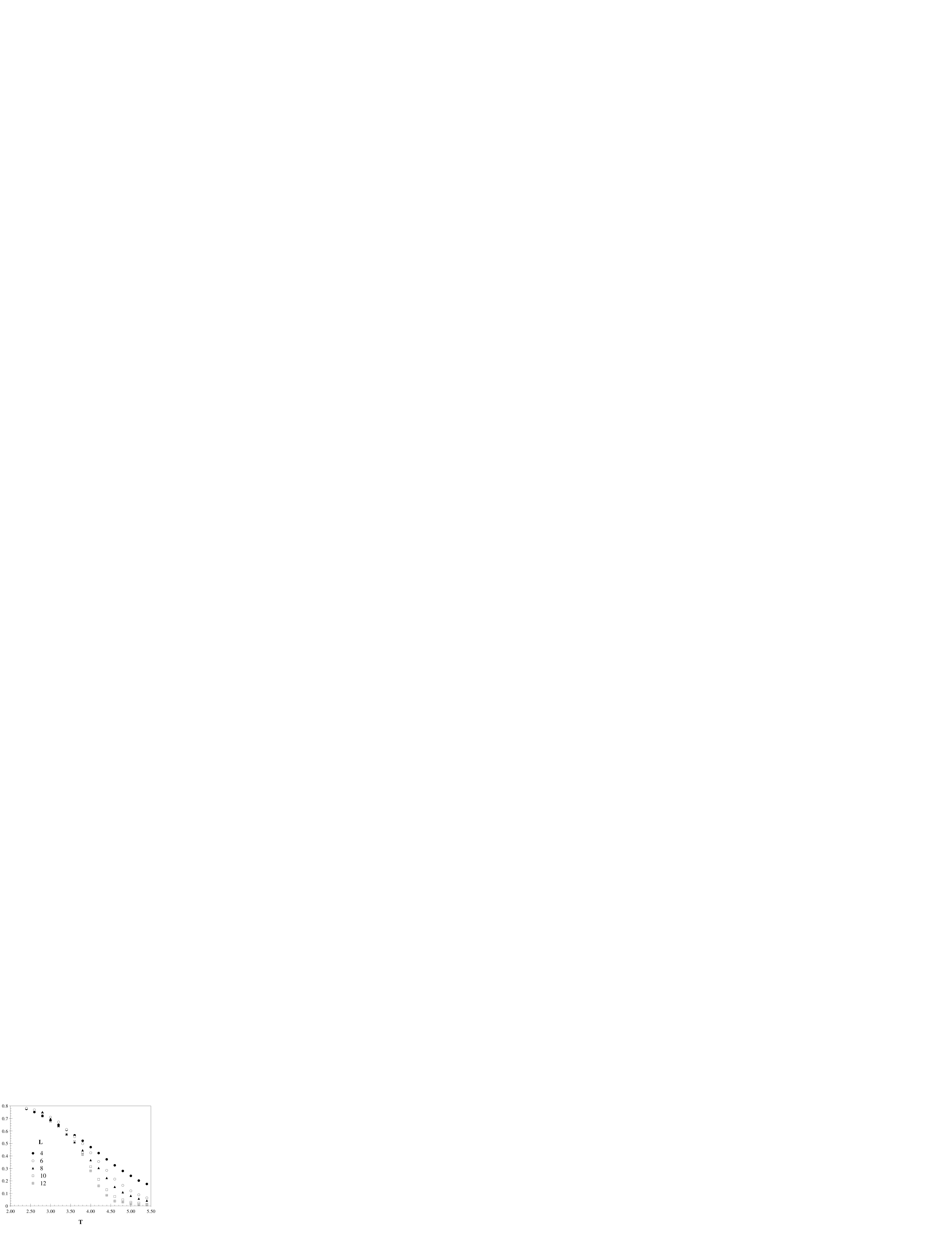
Figure 1: The Binder parameter $g(T)$ as a function of the temperature $T$ for different lattice sizes.

From the large lattice results (see section (4)) we can use the values $T_{c}=3.27$ and $\gamma=2.4$ (see (36)) and $\eta\sim 0$ (see (36)) to check the consistency of the finite size behavior with a finite $T$ transition. In fig. (2) we plot $\frac{\chi_{o}}{L^{2}}$ versus $(T-T_{c})\,L^{\frac{1}{\nu}}$. The data collapse on a single curve, showing a good scaling behavior, on both sides of $T_{c}$. It is already clear from these first data (illustrated in figures (1) and (2)) that it will be exceedingly difficult to distinguish between the two candidate critical (with $T_{c}=0$ or $T_{c}\not=0$) behaviors.

Figure 2: The scaled overlap susceptibility $\frac{\chi_{o}}{L^{2}}$ versus the scaled reduced critical temperature $(T-T_{c})\,L^{\frac{1}{\nu}}$.

To understand better what is happening in the pseudo-critical region, for $T$ close to $3.3$, it is interesting to apply to the model a magnetic field $h$. We expect $q$ to scale as $h^{\frac{2}{\delta}}$. $\delta$ is related to $\eta$ by the hyper-scaling relation

$$\delta=\frac{d+2-\eta}{d-2+\eta}\ .$$ (21)

In presence of $h$ the correct definition of the overlap susceptibility requires subtraction of the connected part, i.e.,

$$\chi_{o}\equiv\lim_{V\to\infty}V(\overline{\langle q^{2}\rangle}-\overline{\langle q\rangle}^{2})\ .$$ (22)

For a finite $T$ phase transition the scaling relation (17) is still satisfied, but now (we are sitting at $T_{c}$) $\xi$ diverges like

$$\xi(h)\sim h^{-\frac{2(\delta+1)}{d\delta}}\ .$$ (23)

(23) only depends on the critical exponent $\eta$. Once we have measured $T_{c}$, and established that a finite $T$ phase transition exists, we can use (23) to find $\eta$.

It turns out that the correct overlap susceptibility we have just defined in (22) is not a good observable for checking scaling. It depends on the first moment of $\langle q\rangle$ that is affected by strong finite size corrections. This is because the region of negative overlaps with $q<0$ is only suppressed in the infinite size limit. We have found preferable to study the behavior of the non-subtracted $\overline{\langle q^{2}\rangle}$, i.e., of the overlap susceptibility defined in absence of $h$ divided times the volume. Here we expect the scaling (17) divided times $L^{3}$, i.e., a scaling with $L$ with the power $-(1+\eta)$.

We have run numerical simulations in presence of a magnetic field. In figure (3) we show $\overline{\langle q^{2}\rangle}$ for several lattice sizes $L=5,7,9,11,13$ and different values of the magnetic field (ranging from $h=0$ up to $h=1.5$). Again we find consistency with $T_{c}=3.27$. The preferred value for $\eta$ is negative and close to $-0.1$. Let us stress that all the finite size scaling fits are not giving very precise predictions. There are many free parameters, and that makes the fitting procedure questionable. Still we should note that all the exponents we find, when assuming a finite $T$ transition, are fully compatible with the ones found for the $r=1$ model in the previous work of references [2, 3, 4, 5].

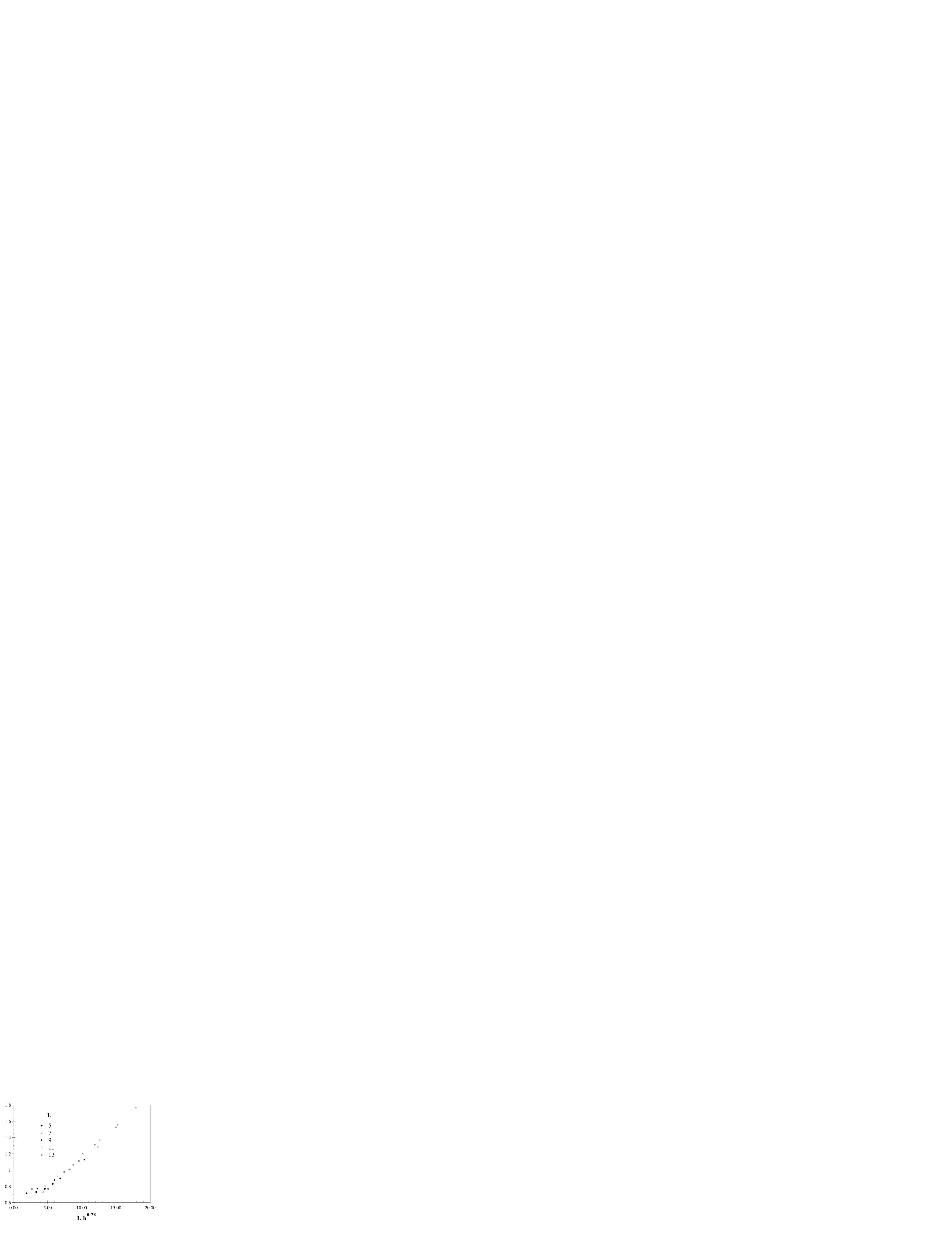
Figure 3: The rescaled $\langle q^{2}\rangle$ as a function of the rescaled applied magnetic field, for different lattice sizes.

As we already hinted the finite size scaling results are also compatible with a $T=0$ singularity. We will use the best value (45) of the parameters defined in (44). In figure (4) we show the rescaled susceptibility $\chi_{o}$ (again without magnetic field, now) for the different lattice sizes. The curves for different lattice sizes scale tremendously well, and the comparison with figure (2) is instructive. This is, as we will discuss in the following, fully compatible with the results obtained for the large lattice size, in a regime where $\xi>>L$.

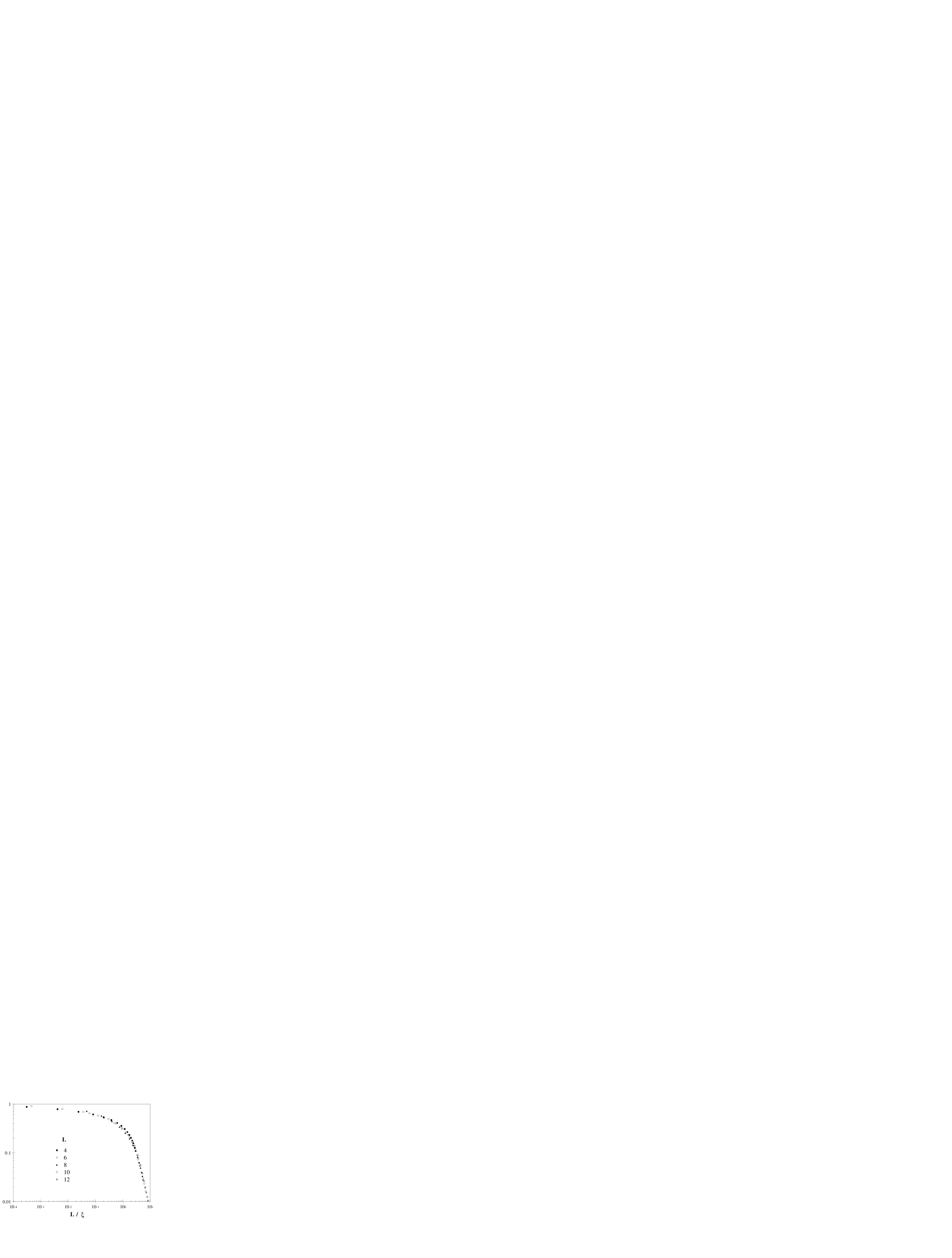
Figure 4: The rescaled $\chi_{o}$ as a function of $\frac{L}{\xi}$. This scaling is compatible with a singularity at $T=0$.

If the transition is at $T=0$ the usual scaling laws imply that the correlation function at large distance behaves as $x^{-\zeta}$, with $\zeta=d-2+\eta$. When the ground state is not degenerate the $T=0$ correlation function goes to a constant value at large distance, implying $\zeta=0$ and in $3d$ $\eta=-1$. The value we estimate for $\eta$ turns out to be not so close to $-1$, and using $\eta=-1$ does not make our curves to scale.

Here we see two options. One possibility is that $\zeta\not=0$ in $3d$ Ising spin glasses (our best fit is close to $\zeta\sim.6$). This possibility cannot be excluded. For example in $2d$ [5] $\zeta$ is estimated to be in the range $.2\sim.3$. In our case, where the coupling constants $J$ take the values $\pm 1$, the ground state is highly degenerate, and there are no general a priori reasons for $\zeta=0$ to hold (however it has been suggested in [13] that at the lower critical dimension we expect indeed $\zeta=0$). The other possibility is that to get good scaling for $\eta$ we have to go at lower values of $T$. Here we have been obliged to seat at not too low $T$’s and it is quite possible that the value of $eta$ in this temperature range is quite different from its zero temperature limit.

In figure (5) we have tried to show the scaling behavior in a suggestive form. We plot $\frac{\chi_{o}(L)}{\chi_{o}(\infty)}$ as a function of $L/\xi$ for the different lattice sizes. The values of $\chi_{o}(\infty)$ and $\xi$ are those discussed in the next sections and computed on very large lattices (which we judge to be free from systematic errors in our statistical precision). The data smoothly collapse on a single curve.

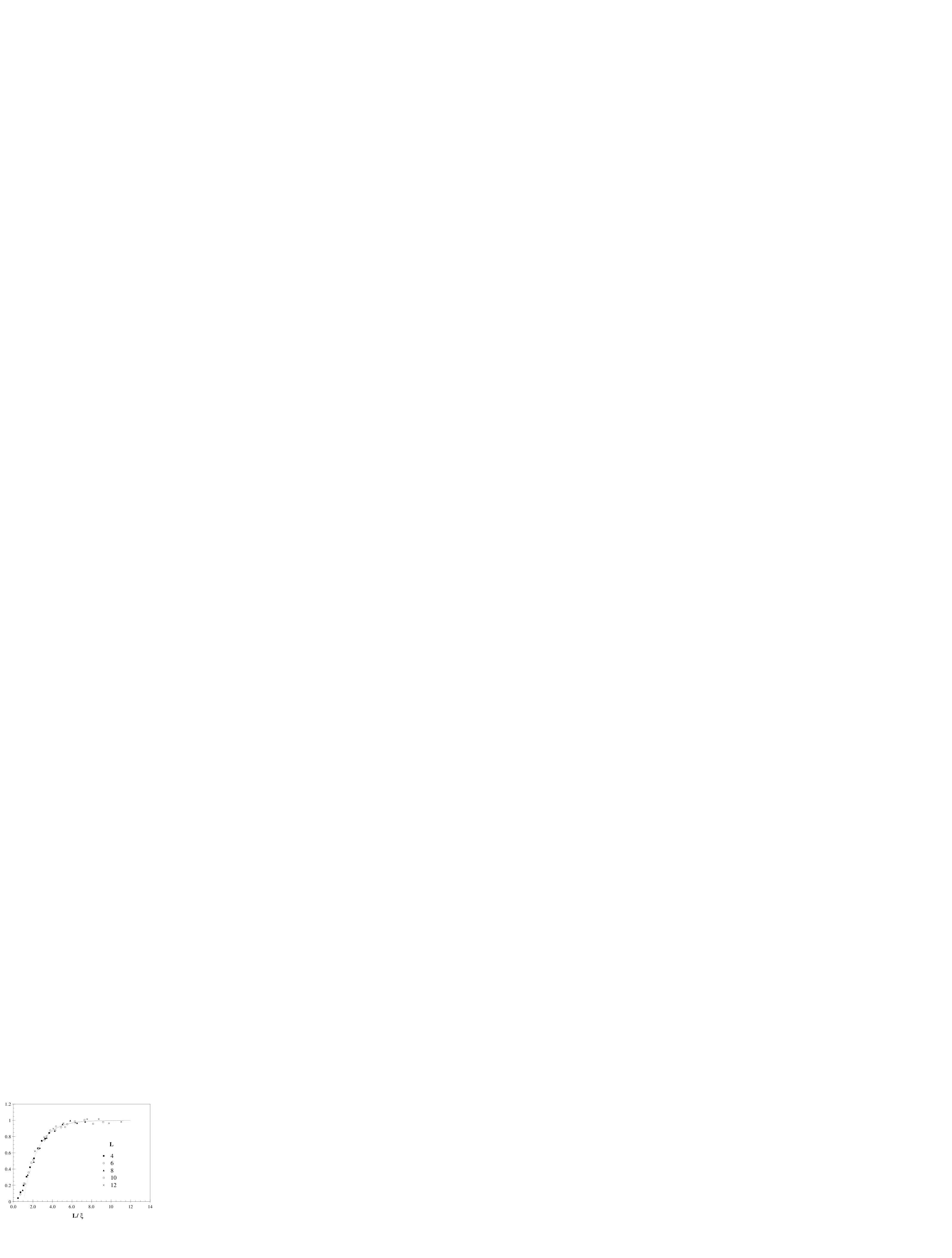
Figure 5: The overlap susceptibility divided times the asymptotic large lattice value (which we denote here by $\chi_{o}^{*}$) versus $\frac{L}{\xi}$. The line is the best fit to the form (31).

From these data it is not clear if the $3d$ Ising spin glass undergoes a finite $T$ phase transition (and mainly the puzzling behavior of Binder cumulant seems to point toward something different). If we assume a finite $T_{c}$ our predictions for the critical exponents agree with those reported in the literature (for the first neighbor cubic lattice model).

Though high temperature expansions predict a finite temperature transition (which agrees with that found in numerical simulations) we consider the compatibility of our data with a $T=0$ phase transition serious (and we will discuss this kind of evidence in more detail in next section, when discussing our large lattice results).

As we have already remarked the behavior of the Binder cumulant below $T_{c}$ is different from what happens in normal spin systems. It is also very different from what one measures in spin glasses in high dimensions, and a few more comments are maybe in order. Let us consider what happens in the usual ferromagnetic Ising case, by defining the function

$$g(T)\equiv\lim_{L\to\infty}g(T,L)\ ,$$ (24)

where here $g(T,L)$ is defined in terms of the moments of the order parameter $m$, the total magnetization of the system. In this non-disordered case we have that

$${\rm for}\ T<T_{c}\ g(T)=1\ ,\ {\rm for}\ T>T_{c}\ g(T)=0\ .$$ (25)

Moreover the quantity $g_{c}\equiv g(T_{c})$ is a function of the dimensionality of the system. It increases when the dimension decreases, and goes to $1$ at the lower critical dimension.

The situation is different in spin glass models. In this case in the mean field approximation $g(T)$ is not trivial at low temperature. One finds that below $T_{c}$

$$g(T)=\frac{3}{2}-\frac{1}{2}\frac{\int dx\ q(x)^{4}}{\bigl{(}\int dx\ q(x)^{2}\bigr{)}^{2}}=\frac{3}{2}-\frac{1}{2}\frac{\int dP(q)\ q^{4}}{\bigl{(}\int dP(q)\ q^{2}\bigr{)}^{2}}\ .$$ (26)

Using the mean field expression for the dependence of $q(x)$ over $T$ one finds that

$$g_{-}\equiv\lim_{T\to T_{c}^{-}}g(T)=1\ ,$$ (27)

but the function $g(T)$ is non trivial. The statement $g\not=1$ coincides with the fact that the $P(q)$ is not equal to a $\delta$-function, and implies replica symmetry breaking. In the mean field approximation no closed formula exists for $g$, however one finds that qualitatively $g$ behaves as

$$1-A\frac{T}{T_{c}}(1-\frac{T}{T_{c}})\ .$$ (28)

In other words $g(T)$ vanishes linearly both at zero temperature and at the critical temperature. For $T>T_{c}$ one still finds that $g(T)=0$. Below the upper critical dimension ($d^{(u)}_{c}=6$) according to the prediction of ref. [13] $g_{-}$ becomes different from $1$. Slightly below $d=6$ the function $g(T)$ is not monotonous, but it is possible that it becomes monotonous at sufficient low dimensions, i.e., near three dimensions. It is tempting to conjecture that near the critical dimension one finds that $g_{c}$ becomes close to $g_{-}$. It is difficult to assess quantitatively the values of these two quantities. If we use our best estimate for $T_{c}$ we find $g_{-}\simeq(.65\pm.05)$, and a very similar value for $g_{c}$. We can only tentatively conclude that:

• The $L$ independence of $g(L,T)$ in the (pseudo)-low temperature phase and the fact that $g(L,T)$ is different from $1$ is a clear signal that replica symmetry is effectively broken in this region. Obviously if there is no finite $T$ phase transition this symmetry breaking will eventually disappear for very large lattices, but it will correctly describe the physics of the system for large lattices with $L$ smaller than the exponentially large correlation length $\xi$.

• The shape of the function $g(T)$ is in qualitative agreement with the predictions of the renormalization group and it suggests that the lower critical dimension is close to $3$ (and very probably exactly $3$).

Let us now discuss in some detail the form of finite size effects. This is very interesting, mainly since we have to plan larger scale numerical simulations, and we want to be sure to optimize the use of our computer time. We will describe here the strategy that should eventually lead us to a numerical simulation in which we can establish in a clear way which kind of singularity the $3d$ Ising spin glass undergoes. For lattice sizes much larger than the correlation length one finds that (in presence of periodic boundary conditions) the finite volume corrections are exponentially small. The leading correction can be computed in perturbation theory, giving:

$$\chi_{o}(L)=\chi_{o}(\infty)\bigl{(}1-{\cal C}\ \xi^{3}\lambda^{2}e^{\frac{-L}{\xi}}\bigr{)}\ ,$$ (29)

where $\cal C$ is some computable constant, and $\lambda$ is the coupling constant of a $\phi^{3}$-like interaction in a field theoretical framework. Close to the critical point the usual scaling laws imply that quantity $\xi^{3}\lambda^{2}$ goes to a constant. So we obtain:

$$\chi_{o}(L)=\chi_{o}(\infty)\bigl{(}1-{\cal C}\ e^{\frac{-L}{\xi}}+O(e^{\frac{-2L}{\xi}})\bigr{)}\ .$$ (30)

We have fitted our data for the correlation length on small lattices, divided over the large lattice result, as

$$\frac{\chi_{o}(L)}{\chi_{o}(\infty)}\simeq(1-{\cal C}e^{\frac{-L}{\xi}})\ .$$ (31)

The best fit works very well. We show it in figure (5). For a finite temperature transition $\cal C$ is important. It is universal and in principle it can be computed in a field theoretical renormalization approach.

These data are relevant since they are crucial for planning simulations free of finite size effects on large lattices. We see that if we require finite size effects to be smaller than $1\%$ we need to have $L/\xi>6$, while to reach a $10\%$ accuracy we can accept $L/\xi>3.5$.

In a similar way it is interesting to compute

$$K={\overline{\chi_{o}^{2}}-\overline{\chi_{o}}^{2}\over\overline{\chi_{o}}^{2}}\ .$$ (32)

The quantity $K$ measures the susceptibility system to system fluctuations. We expect it to have similar properties to the Binder cumulant $g$. In particular at low temperatures mean field predicts that

$$K=\frac{1}{3}\Bigl{(}{\int dx\ q(x)^{4}\over(\int dx\ q(x)^{2})^{2}}-1\Bigr{)}\ .$$ (33)

In other words mean field theory predicts that

$$\overline{\langle q^{4}\rangle-\langle q^{2}\rangle^{2}}=2\bigl{(}\overline{\langle q^{2}\rangle^{2}}-\overline{\langle q^{2}\rangle}^{2}\bigr{)}\ .$$ (34)

The size dependence of $K$ can be used to estimate the number of different realizations of the quenched disorder we need to extract an accurate value of $\chi_{o}$.

The measurament of $K$ is rather delicate because for each system we must know the value of $\langle q^{2}\rangle$ with high accuracy. In figure (6) we plot $K$ as a function of $\frac{L}{\xi}$ for $L=6$.

Figure 6: $K$ as a function of $\frac{L}{\xi}$.

4 Large Lattice Results and Discussion

Our large lattice runs have been done on a $64\times 64\times 128$ lattice, on the $8192$ processor DECmpp at Syracuse NPAC. We have always studied the evolution of two replica of the system in the same realization of the quenched disorder. In this way we have been able to compute the overlap between two replica.

Figure 7: $\chi_{o}$, the overlap susceptibility, for the two realizations of the random couplings.

We have studied the behavior of the system for two different realizations of the quenched random couplings. We give in table (1) the details about the two series of runs (the number of millions of sweeps is for each of the two replica we studied in a given coupling realization).

$T$	Sample $1$	Sample $2$
$6.0\to 4.4$	$0.005+0.5$
$4.3\to 3.8$	$0.5+2.0$	$0.5+2.0$
$3.7$	$0.5+4.5$	$0.5+14.5$
$3.6$	$2.5+9.0$	$2.5+30.0$

Table 1: For the two different realizations of the couplings, the number of millions of MC sweeps we used. We give the number of thermalization sweeps, plus ($+$) the number of sweeps used for measuring.

We studied two different realizations of the random noise mainly to check the size of the fluctuations of $\chi_{o}$. We wanted to be sure that even for our $T$ point closer to criticality ($T=3.6$) sample to sample fluctuations are not too dramatic. In fig. (7) we show that in the worst case the two results for $\chi_{o}$ deviate of less then two standard deviation (in this and in the following figures the smooth lines just join the Monte Carlo data points with straight segments). But we know from our binning analysis that the error we quote is probably slightly underestimated at the lower $T$ values. So we find this result reassuring, consistent with the serious critical slowing down that we are observing and with critical fluctuations.

Figure 8: As in fig. (7), but the two internal energies.

The internal energies of the two systems are completely compatible (fig. (8)), as it is the specific heat (which we measure both from equilibrium fluctuations and from the $T$ derivative of the internal energy, fig. (9)). We feel confident that on the $64\times 64\times 128$ lattice results do not vary much with the sample, and in the following we will discuss results averaged over the two realizations of the quenched disorder.

Figure 9: As in fig. (7), but the specific heats. The point with a large statistical noise are from the energy fluctuations, while the ones with a smaller noise are from $T$ derivatives of the internal energy.

We have estimated statistical errors by a binning analysis. We have systematically blocked the data in coarser and coarser sub-samples, to check statistical independence of the configuration groups eventually used for the final error analysis. Always but for the two lower $T$ values ($3.6$ and $3.7$) we have reached a very reliable estimate of the true statistical error. In the two last cases the error seems stabilizing under binning, but the evidence is less compelling, and we would allow for a possible small underestimation of the statistical error (of less, say, than $50\%$).

For $T$ going from $6.0$ down to $4.4$ we present errors based on $9$ blocks of order of $50,000$ configurations (the actual measurements were taken just once in $200$ sweeps). From $4.3$ down to $3.8$ we have $9$ blocks of order $400,000$ configurations each. At $T=3.7$ we have used $5$ blocks of $3\times 10^{6}$ configurations, and at $T=3.6$ $6$ groups of $6.5\times 10^{6}$ configurations.

In fig. (10) we plot the final overlap susceptibility, averaged over the two coupling realizations, as a function of the temperature $T$.

Figure 10: The overlap susceptibility, averaged over the two different samples.

Our main goal has been trying to establish (or disprove) the existence of a finite $T$ phase transition for the $3d$ spin glass model under study. Since correlation times diverge very fast when approaching the low temperature region (or $T_{c}^{+}$, if it exists), we are not in an easy situation. On a large lattice we have to look at data far away in the warm phase (the one we can check and trust have thermalized), and try to decide which kind of critical behavior they have.

At first we have tried fitting $\chi_{o}$ with a power divergence at the critical temperature $T_{c}$, i.e.,

$$\chi_{o}\simeq 1+\frac{A^{\chi}_{p}}{(T-T_{c})^{\gamma}}\ ,$$ (35)

where the subscript $p$ stands for power fit. We show in fig. (11a) our best fit, obtained by using all the data points shown in the figure. The results are

$$A^{\chi}_{p}=19.3\pm 1.1,\ T_{c}=3.27\pm.02,\ \gamma=2.43\pm.05\ .$$ (36)

We do not attach much significance to the statistical errors quoted here. They are reasonable estimates of a standard fitting routine, but not the result of a detailed study of a very complex $3$-parameter fit. We will see in a moment that the main issue here is not the statistical error, but the systematic error, which is, as far as we can judge from the present data, infinite (see later).

Obviously one would like to select a $T$ region that would allow exposing a good scaling behavior (and to be obliged from the fit to discard a high $T$ region where scaling corrections are important and a region close to $T_{c}$ where finite size effects become sizeable). This would amount, in some sense, to find at least the size of the first corrections to scaling. In the present case we have to compromise on the quality of the results in (36), which is, still, reasonably good. We have checked that by fitting only points close to $T_{c}$ we get results that are not so different from the ones given in (36). For example if we fit from $T=5.0$ down to $T=3.6$ we obtain $\gamma=2.67\pm.06$, and $T_{c}=3.20$.

Let us repeat that here the problem will turn to be mainly the systematic error.

The second functional behavior we have tried assumes no critical point, but an essential singularity at $T=0$. We have first tried the form

$$\chi_{o}\simeq A^{\chi}_{e}(e^{(\frac{B^{\chi}_{e}}{T})^{P}}-1)+C^{\chi}_{e}\ ,$$ (37)

where the subscript $e$ stands for exponential fit. The power $P$ turned out to be very close to $4$ (also for the exponential fit to the correlation length $\xi$, see later). We have tried fits with different fixed power $P$, and for the fit to $\chi_{o}$ (the fit to $\xi^{(1)}$ has a larger indetermination, see later) we find that a power of $3$ or $5$ gives clear worse results than a power $4$. So we have eventually used the $3$-parameter fit to the form

$$\chi_{o}\simeq A^{\chi}_{e}(e^{(\frac{B^{\chi}_{e}}{T})^{4}}-1)+C^{\chi}_{e}\ ,$$ (38)

which gives results

$$A^{\chi}_{e}=1.67\pm.05,\ B^{\chi}_{e}=5.38\pm.01\ ,C^{\chi}_{e}=1.28\pm.05,\$$ (39)

The best fit is very good, and we show it in fig. (11b), on the right. The $\chi^{2}$ is much better than for the power fit ($12$ versus $29$ with some slightly arbitrary normalization).

Figure 11: The overlap susceptibility, same than in fig. (10). Here the continuous lines are the results of the best fits. In fig. (11a), on the left, the result of the power fit to the form (35), and in fig. (11b), on the right, the result of the power fit to the form (38).

The divergence of the correlation length as a function of $(T-T_{c})$ gives, if a phase transition exists, the exponent $\nu$. We have repeated here the analysis we have discussed for $\chi_{o}$. In fig. (12) we give $\xi^{(1)}$ (we have defined before) as a function of $T$. $\xi^{(0)}$ is always compatible with $\xi^{(1)}$, but has a larger statistical error.

Our estimator for $\xi^{(1)}$ is defined by taking the weighted average of the effective mass estimator at distance $d$

$$\tilde{m}(d)\equiv\log(\frac{C^{(1)}(d)}{C^{(1)}(d+1)})\ ,$$ (40)

for $d$ going roughly from $\xi$ to $2\xi$. In this way we are making systematic effects (coming from small distance contributions) and statistical error small. A typical fitting window is $d$ from $2$ to $3$ at large $T$ down for example to $8$ to $15$ at $T=3.7$. We have estimated errors by using a standard binning plus jack-knife procedure. Our conclusions about the statistical significance of the sample coincide with the ones we have drawn for $\chi_{o}$.

Figure 12: The correlation length $\xi^{(1)}$, averaged over the two different samples. The continuous line is here only to join neighboring points.

Also in this case we have tried a power fit and an exponential fit. For the power fit we used the form

$$\xi^{(1)}\simeq\frac{A^{\xi}_{e}}{(T-T_{c})^{\nu}}\ ,$$ (41)

with the result

$$A^{\xi}_{e}=2.73\pm.11,\ T_{c}=3.24\pm.03,\ \nu=1.20\pm.04\ .$$ (42)

Even if the results are very reasonable, the fit is not good (as shown in fig. (13a), on the left). The $\chi^{2}$ is very high ($\simeq 120$), and the points close to $T_{c}$ are the one that do not fit (very dangerous caveat!). Still, if we take these data seriously, we have to notice that $T_{c}$ is the same we estimated by using $\chi_{o}$, and that by means of the scaling relation

$$\gamma=\nu(2-\eta)$$ (43)

we get $\eta\simeq 0$.

The exponential fit has the form

$$\xi\simeq A^{\xi}_{e}(e^{(\frac{B^{\xi}_{e}}{T})^{4}}-1)+C^{\xi}_{e}\ ,$$ (44)

and gives

$$A^{\xi}_{e}=1.41\pm.05,\ B^{\xi}_{e}=4.21\pm.02\ ,C^{\xi}_{e}=.46\pm.01,\ .$$ (45)

Such best fit is very good, and we show it in fig. (13b). The $\chi^{2}$ is $4$ times smaller than for the power fit. This fit is by far a better fit than the fit to a power law behavior.

Figure 13: The correlation length, same than in fig. (12). Here the continuous lines are the results of the best fits. In fig. (13a), on the left, the result of the power fit to the form (41), and in fig. (13b), on the right, the result of the power fit to the form (44).

For $\xi$ the evidence for the power in the exponential being $4$ is less compelling than for $\chi_{o}$. Here fit with power $2$, $3$ or $5$ are acceptable, also if the $\chi^{2}$ is minimum at power $4$ (or $5$, which gives a very similar fit. For power $3$ a small decrease in quality is already apparent).

In fig. (14) we show the data for

$$Z_{0}\equiv\chi_{o}m^{2}\ ,Z_{1}\equiv g_{1}m\ ,$$ (46)

from the data we have already shown for $m$, the inverse correlation length. We expect both quantities to diverge as $m^{\eta}$ in the small $m$ limit. Both quantities can are well fitted with a power law with $\eta\sim-.25$.

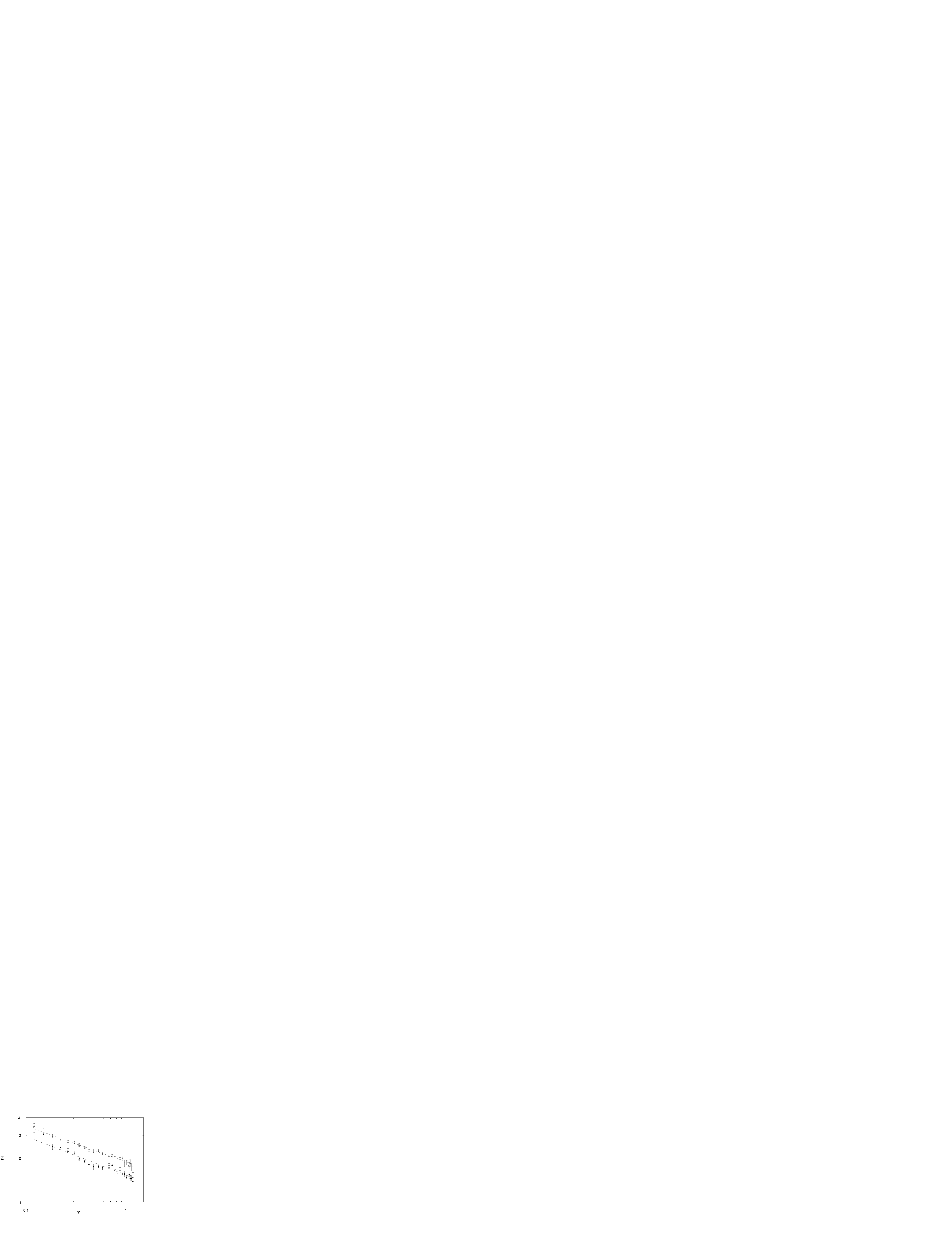
Figure 14: The quantities $Z_{0}$ (lower curve) and $Z_{1}$ (upper curve) as function of $m$ in a logarithmic scale.

An independent way to measure $\eta$ is to study directly the data for the correlation function $G^{(1)}$. At large distances the data can be fitted as

$$\frac{{\cal Z}(\beta)}{r}e^{-mr}\ .$$ (47)

${\cal Z(\beta)}$ seems to diverge close the critical temperature, with a very small power $\sim m^{-.1}$, making this estimate of $\eta$ quite different from the previous one. The discrepancy among the two estimates of $\eta$ is likely to be related to the small asymptotic value of $\eta$.

As a check we have analyzed the data for the correlation function

$$C(s)\sim\frac{rG^{(1)}(r)}{{\cal Z}(\beta)}\ ,$$ (48)

in the scaling region as function of $s\equiv\frac{r}{\xi}$. The fact that the exponentially decaying fits to the correlation function are good implies that for $s>1$ the function $C(s)$ is well approximated by $e^{-s}$. At small values of $s$ the function should go to zero as $s^{\eta}$. Alas, since we cannot reach very small values of $s$ it is difficult to use this method to get a precise determination of $\eta$.

Let us insist on the difficulty in reaching a definite conclusion about the critical regime by presenting some more fits (figures (15) and (16). Here we are analyzing the overlap susceptibility $\chi_{o}$ as function of $\beta$. In fig. (15) we show the best fit to the form (35) with the parameters given in (36) (with a transition at a critical temperature), and we superimpose a second fit of the form

$$\log(\chi_{o})\ =\ A\ e^{(B\beta)}\ ,$$ (49)

with $A=.085$ and $B=15.16$. Again, although the two functional forms imply a very different critical behavior, in the region we have studied they are indistinguishable.

Figure 15: Two fits to the data for the susceptibility $\chi_{o}$, as a function of $\beta$, according to equations (35,49).

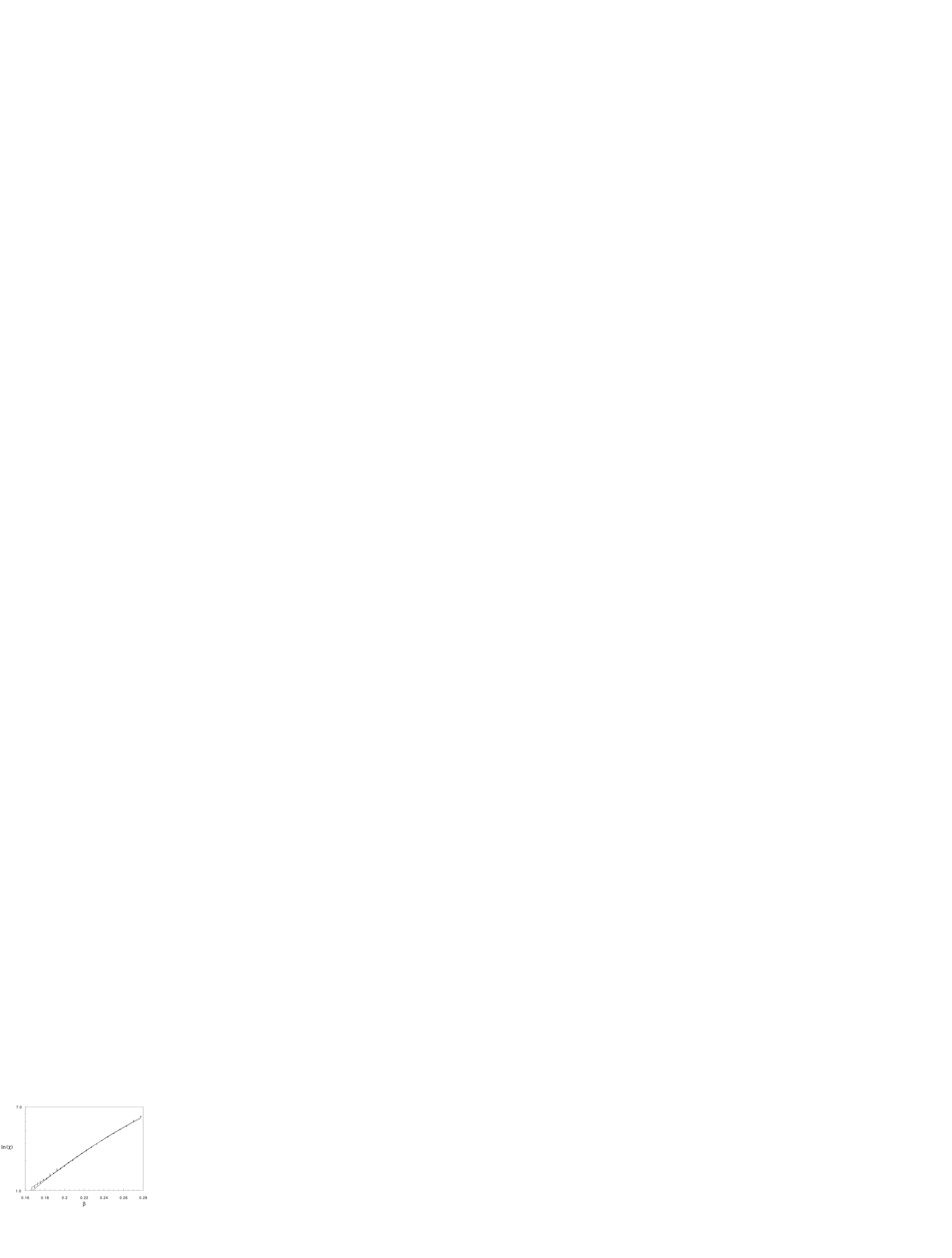
Figure 16: Two fits to the data for the susceptibility $\chi_{o}$, as a function of $\beta$, according to equation (50).

We can try more. A similar phenomenon is displayed in fig. (16). Here we show dependencies that imply a transition at zero temperature:

$$\log(\chi_{o}) = A\beta^{\omega}$$

$$\log(\chi_{o}) = A+B\beta+C\beta^{2}\ .$$ (50)

In the first best fit we find $A=383$ and $\omega=3.33$, while in the second best fit we get $A=5.9$, $B=-69.8$ and $C=246$. $\omega$ turns out to be not so far from $4$, as we already remarked.

The four fits all give reasonable results. It is impossible to use the data to reject one of them. Of course we could choose the one with smallest $\chi^{2}$, but this procedure may give an incorrect answer since we have neglected sub-asymptotic terms, inducing an systematic error which are out of control.

From these data, we tend to conclude we have a hint for the absence of a phase transition in the $3d$ spin glass. If on the contrary such a phase transition is present, than we have given a reasonably precise estimate of the critical exponents.

5 Conclusions

We believe we have pointed out an open problem that in recent papers was quoted as solved. Nowadays it is usually said that the existence of a phase transition is established. For example ref. [7] about aging phenomena (see [8] for more aging papers) claims that it is common lore that $3d$ spin glasses undergo a finite $T_{c}$ phase transition. It does not seem to us that the existence of a phase transition is well established at all.

The possibility of $3$ being the lower critical dimension is appealing. We have in mind a scenario where the predictions of the mean field theory describe fairly the behavior of the system down to $d=3$, where the transition disappears. In no cases, as it is sensible to expect, the system behaves as a normal ferromagnet. At low $T$ in $3d$ the system is reminiscent of the mean field picture up to a critical length which is function of $T$, and diverges at $T=0$.

As it was noted many years ago in ref. [14] at the lower critical dimension we expect $\frac{1}{f}$ noise for the power spectrum of the magnetization, that agrees with what has been observed experimentally [15].

It is clear that there is an apparent critical temperature. Close to this pseudo-$T_{c}$ the correlation length becomes so large that it cannot be measured on the lattice sizes that are normally studied. Below such temperature the system behaves as if it is in the low temperature phase, irrespectively of the existence of the transition (think about the $1d$ normal Ising model for low values of $T$).

The only way to disprove the existence of a transition at finite temperature would be to show that the data for the susceptibility and the correlation length cannot be fitted with power law singularities at finite temperature. On the contrary to present an evidence for a transition at finite temperature one should show that the data can be fitted as power law singularities and cannot be fitted with functions having only singularities at zero temperature. Our data, as well those from the very long simulations of Ogielski and Morgenstern [2, 4], can be fitted in both ways. As we already said, we do not think that we can discriminate the two admissible behaviors from the value of the chi-square $\chi^{2}$, i.e., of the quality of the fit, especially in an approach where corrections to scaling have been neglected. Unfortunately in absence of clear predictions about the low temperature behavior it is difficult to exclude the possibility of a transition at $T=0$.

To visually discriminate among the two possibilities we plot in figure (17) the quantity

$$\Gamma\equiv\frac{d\beta}{d\log(\chi_{o})}\ ,$$ (51)

versus $\tau\equiv\log(\chi_{o})$. A finite $T$ transition implies that

Figure 17: $\Gamma$ versus $\tau$ (see the definitions in the text).

$$\Gamma\simeq e^{-A\tau}\ ,$$ (52)

with $A=1/\gamma$, while a transition at $T=0$ with a divergence of the form $\exp(\beta^{\omega})$ implies

$$\Gamma\simeq\frac{1}{\tau^{B}}\ ,$$ (53)

with $B=1-{1\over\omega}$. $B=1$ corresponds to an $e^{(e^{\beta})}$ behavior. Our best fits give $A=.29$ and $B=.86$. The data are noisy at high temperature (low $\tau$). Clearly it is difficult to select one fit, especially since we have neglected corrections to scaling. Data seems to prefer a straight line with a coefficient not far from one, but we are unwilling to rely on this kind of evidence.

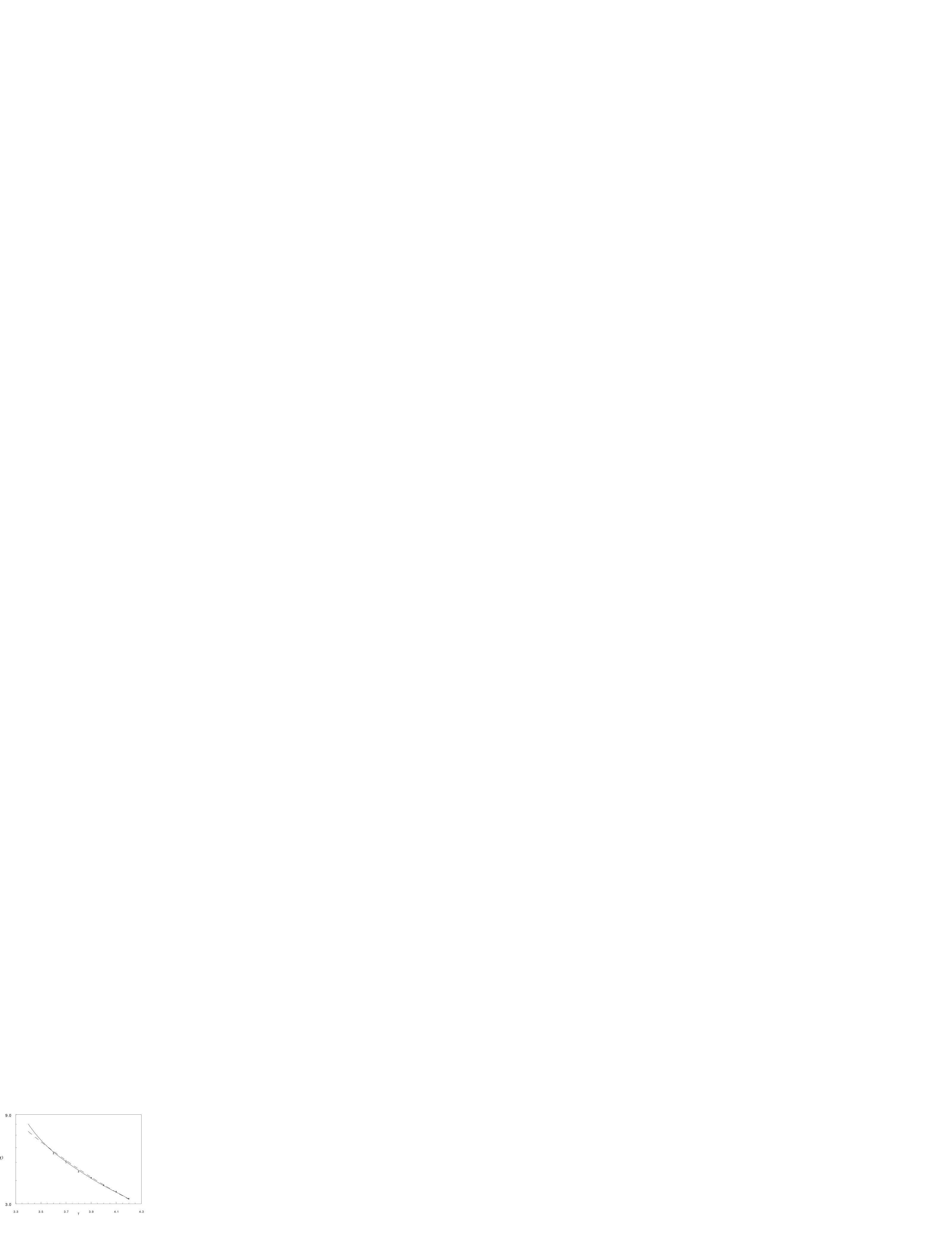
Figure 18: $\log{\chi_{o}}$ versus $T$. Fit $1$ (continuous line) is to a power law singularity, as in eq. (35) fit $2$ (dashed line) has a $T=0$ singularity, as in eq. (49).

What can be done with a better numerical simulation? To get a hint we have extrapolated two typical fits at a reasonable low $T$. We show them in fig. (18). We have considered a simple power singularity at $T\not=0$, and a divergence at $T=0$ of the form $e^{Ae^{B}}$. From our present best fits we can deduce that at, say, $T=3.4$, we would be able to discriminate. If the data would be really following the finite $T$ singularity scenario (first case), the strong increase of the susceptibility could not be fitted by the double exponential scenario, and the zero temperature transition should be refuted.

In the opposite case, where the hypothetical data would follow a form of the second kind (a double exponential singularity at $T=0$) we find that a power fit would still be a good fit, but with a larger value of $\gamma$ and smaller value of $T_{c}$. This variation of the value of the best fit parameters with the temperature interval used for the fitting would then be taken as good evidence for the existence of a zero temperature transition.

If the double exponential singularity behavior is correct, the correlation length should increase of a factor about $2.5$ when going from $T=3.6$ to $T=3.4$. That means that a reliable estimate will be possible on $128^{3}$ lattice, only slightly larger of what we used here, and not out of reach of the present technology. An increase of the computer time of more than one order of magnitude seems unfortunately necessary, but this is also a reasonable goal. Such a computation seems possible in a not too far away future.

It is also possible that a careful analysis of the model at low $T$ could allow to show the absence of a phase transition. In this case it would be essential to identify the renormalization group flow away from the zero temperature fixed point.

References

- [1] M. Mezard, G. Parisi and M. A. Virasoro, Spin Glass Theory and Beyond (World Scientific, Singapore 1987); G. Parisi, Field Theory, Disorder and Simulations (World Scientific, Singapore 1992).
- [2] A. T. Ogielski and I. Morgenstern, Critical Behavior of Three-Dimensional Ising Spin-Glass Model, Phys. Rev. Lett. 54 (1985) 928.
- [3] R. N. Bhatt and A. P. Young, Search for a Transition in the Three-Dimensional Ising Spin-Glass, Phys. Rev. Lett. 54 (1985) 924.
- [4] A. T. Ogielski, Dynamics of Three-Dimensional Ising Spin-Glasses in Thermal Equilibrium, Phys. Rev. B32 (1985) 7384.
- [5] R. N. Bhatt and A. P. Young, Numerical Studies of Ising Spin Glasses in Two, Three and Four Dimensions, Phys. Rev. B37 (1988) 5606.
- [6] R. E. Hetzel, R. N. Bhatt and R. R. P. Singh, Europhys. Lett. 22 (1993) 383.
- [7] H. Rieger, cond-mat/9303048, J. Phys. A (Math. Gen.) 26 (1993) L615.
- [8] L. F. Cugliandolo and J. Kurchan, Phys. Rev. Lett. 71 (1993) 1; L. F. Cugliandolo, J. Kurchan and F. Ritort, Evidence of Aging in Spin Glass Mean-Field Models, cond-mat/9307001 preprint (July 1993); E. Marinari and G. Parisi, On Toy Aging, cond-mat/9308003 preprint (August 1993), to be published in J. Phys. A Math. Gen..
- [9] G. M. Torrie and J. P. Valleau, J. Comp. Phys. 23 (1977) 187; I. S. Graham and J. P. Valleau, J. Chem. Phys. 94 (1990) 7894; J. P. Valleau, J. Comp. Phys. 96 (1991) 193.
- [10] B. Berg and T. Neuhaus, Phys. Lett. B267 (1991) 249; Phys. Rev. Lett. 68 (1992) 9.
- [11] E. Marinari and G. Parisi, Europhys. Lett. 19 (1992) 451.
- [12] T. Celik, U. Hansmann and B. Berg, Study of Ising Spin Glasses Via Multicanonical Ensemble, cond-mat/9303025 preprint (March 1993), and references therein.
- [13] C. de Dominicis, I. Kondor and T. Temesvari Ising Spin Glass: Recent Progress in the Field Theory Approach, Int. J. Mod. Phys. B7 (1993) 986.
- [14] E. Marinari, G. Paladin, G. Parisi and A. Vulpiani, Noise, Disorder and Dimensionality, J. Physique (France) 45 (1984) 657.
- [15] M. Ocio, H. Bouchiat and P. Monod, J. Phys. Lettres 46 (1985) L647.