Electron-phonon effects on spin-orbit split bands of two dimensional systems

Abstract

The electronic self-energy is studied for a two dimensional electron gas coupled to a spin-orbit Rashba field and interacting with dispersionless phonons. For the case of a momentum independent electron-phonon coupling (Holstein model) we solve numerically the self-consistent non-crossing approximation for the self-energy and calculate the electron mass enhancement $m^{*}/m$ and the spectral properties. We find that, even for nominal weak electron-phonon interaction, for strong spin-orbit couplings the electrons behave as effectively strongly coupled to the phonons. We interpret this result by a topological change of the Fermi surface occurring at sufficiently strong spin-orbit coupling, which induces a square-root divergence in the electronic density of states at low energies. We provide results for $m^{*}/m$ and for the density of states of the interacting electrons for several values of the electron filling and of the spin-orbit interaction.

I Introduction

Prompted by considerable technological interests, the physics of itinerant electrons coupled to spin-orbit (SO) potentials has been the subject of extensive investigations in recent years.prinz ; fabian In materials of interest, the main sources of SO coupling are the Rashba interaction arising from structural inversion asymmetries of low-dimensional structures,rashba and the Dresselhaus interaction present in bulk crystals lacking inversion symmetry.dressel Depending on the material characteristics, one of the above interactions, or even both, may be present, lifting the spin degeneracy of the electron dispersion. When measured at the Fermi level, the resulting energy splitting, $\Delta_{\rm so}$, is commonly used to estimate the strength of the SO interaction.

In narrow-gap III-V semiconductor-based heterostructures, such as GaAs and InAs quantum wells, $\Delta_{\rm so}$ is a few meV, while in II-VI quantum wells $\Delta_{\rm so}$ is greatly enhanced. For example the heavy-hole conduction band of HgTe displays SO splitting values ranging between $10-17$ meV and $30$ meV.zhang ; gui Much stronger SO splittings have been observed in the surface states of metalslashell and semimetalskoroteev ; sugawara , and the corresponding $\Delta_{\rm so}$ may be so large, e.g. $\Delta_{\rm so}\simeq 110$ meV in Au(111),lashell that the possibility of detecting SO split image states has been recently put forward.mclaughlan Other systems displaying giant SO splittings are surface alloys as, for example, Li/W(110),rotenberg Pb/Ag(111),pacile ; ast1 and Bi/Ag(111),astprl or even one-dimensional structures such as Au chains in vicinal Si(111) surfaces.barke For such low-dimensional or structured materials, the SO interaction is of Rashba type, but large SO splittings have been found (or predicted) also in bulk crystals, where the Dresselhaus interaction leads to $\Delta_{\rm so}$ as large as $200$ meV in non-centrosymmetric superconductors CePt₃Si,bauer ; samokhin Li₂Pd₃B, and Li₂P7₃B.togano ; yuan

Such strong SO couplings may possibly have interesting applications in spintronic devices, but represent also a compelling and challenging problem from the theoretical standpoint, in particular when $\Delta_{\rm so}$ is no longer the smallest energy scale in the system, as in III-V semiconductor heterostuctures where $\Delta_{\rm so}\approx 1-5$ meV, but competes in magnitude with other characteristic energy scales such as the phonon frequency or the Fermi energy. From this perspective, systems like the Bi/Ag(111) surface alloy, which shows bands split by about $200$ meV,ast1 ; astprl are particularly promising, given also the alleged possibility of tuning, by Pb doping, the Fermi energy $E_{F}$ to values lower than the SO energy splitting.astold

A few novel and interesting features arising from strong SO splittings have already been investigated theoretically in the literature. For example, in Ref.[chaplik, ] it has been demonstrated that the Rashba SO coupling induces an infinite number of bound states in two dimensions, even for short ranged impurity potentials, while in a recent work we have shown that the superconducting critical temperature of a low-density two-dimensional (2D) electron gas can be significantly enhanced by the Rashba interaction.cgm2007 Both phenomena discussed in Refs.[chaplik, ; cgm2007, ] can be understood in terms of a SO induced topological change of the Fermi surface, which gives rise to an effective reduction of dimensionality of the electronic density of states for $E_{F}$ sufficiently smaller than the SO characteristic energy.

In this paper we analyze the effects of such topological change of the Fermi surface on the electron-phonon (el-ph) problem of 2D systems. In particular, we study one-particle spectral properties and extract the combined el-ph and SO effects on the electronic effective mass $m^{*}$ and on the interacting density of states (DOS). We show that, even for weak or moderate couplings to phonons, the effective reduction of the bare DOS induced by the Rashba interaction leads to a strong increase of $m^{*}$, and to phonon satellite peaks in the interacting DOS, which are typical signatures of an effectively strong el-ph coupling. Due to the two-dimensionality of our model, and to the Rashba type of SO coupling, our results could be relevant for both metal and semimetal surface states, for which the el-ph interaction has been shown to be relevant,sugawara ; gayone ; hofmann ; lashell2 ; kroger and for surface superconductors,gorkov with the hypothesis that pairing is provided by the coupling to phonons.

II Rashba-Holstein model

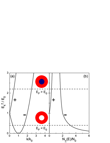
Figure 1: (color online). (a): electron dispersion $E_{k}^{\pm}=\frac{\hbar^{2}}{2m}(k\pm k_{0})^{2}$ for a spin-orbit split electron gas. The energy $E_{0}=\frac{m}{2\hbar^{2}}\gamma^{2}$ is a measure of the spin-orbit interaction and is equivalent to the minimum interband excitation energy for an electron sitting at the bottom of the lower band. The upper and lower horizontal dashed lines indicate the position of the Fermi level for $E_{F}>E_{0}$ and $E_{F}<E_{0}$, respectively. Also shown are the corresponding Fermi circles with occupied states drawn by gray (colored) regions. (b): density of states plotted from Eqs.(6,7).

Two-dimensional quantum wells, with strong and asymmetric confining potentials, and surface states with weak or negligible coupling to the bulk can be satisfactorily represented by the following 2D electron hamiltonian with SO interaction

$$H_{0}=\sum_{\mathbf{k}\alpha}\epsilon_{\mathbf{k}}c^{\dagger}_{\mathbf{k}\alpha}c_{\mathbf{k}\alpha}+\sum_{\mathbf{k}\alpha\beta}\mathbf{\Omega}_{\mathbf{k}}\cdot\mbox{\boldmath$\sigma$}_{\alpha\beta}c^{\dagger}_{\mathbf{k}\alpha}c_{\mathbf{k}\beta}$$ (1)

where $c^{\dagger}_{{\bf k}s}$ ($c_{{\bf k}s}$) is the creation (annihilation) operator for an electron with momentum ${\bf k}=(k_{x},k_{y})$ and spin index $\alpha=\uparrow,\downarrow$. In the above expression, $\epsilon_{{\bf k}}$ is the electron dispersion in the absence of SO coupling, $\sigma$ is the spin-vector operator with components ($\sigma^{x},\sigma^{y},\sigma^{z}$) given by the Pauli matrices, and $\mathbf{\Omega}_{\bf k}$ is a ${\bf k}$ dependent SO pseudopotential arising from the asymmetry in the $z$-direction of the confining potential. Here we consider a linear Rashba model for the SO interaction

$$\mathbf{\Omega}_{{\bf k}}\cdot\mbox{\boldmath$\sigma$}=\gamma(k_{x}\sigma^{y}-k_{y}\sigma^{x}),$$ (2)

where $\gamma$ is the SO coupling constant. Furthermore, we assume that the unperturbed electron band is parabolic, $\epsilon_{{\bf k}}=\hbar^{2}k^{2}/2m$, where $m$ is the band mass of the electron. Apart from a constant shift $E_{0}$ (defined below) which can be absorbed in the chemical potential, the eigenvalues of Eqs.(1) and (2) are:

$$E_{k}^{s}=\frac{\hbar^{2}}{2m}(k+sk_{0})^{2},$$ (3)

where $k=|{\bf k}|$, $s=\pm$ is the chirality number, and $k_{0}$ is the Rashba momentum

$$k_{0}=\frac{m}{\hbar^{2}}\gamma.$$ (4)

The two electron branches $E_{k}^{\pm}$ are plotted in Fig. 1(a) in units of the Rashba energy

$$E_{0}=\frac{\hbar^{2}k_{0}^{2}}{2m}=\frac{m}{2\hbar^{2}}\gamma^{2}$$ (5)

which corresponds to the energy difference between the degeneracy point at $k=0$ and the bottom of the lower band at $k=k_{0}$. In Fig. 1(a) we indicate also the Fermi levels for the $E_{F}>E_{0}$ and $E_{F}<E_{0}$ cases (horizontal dashed lines) which represent two qualitatively different situations. For $E_{F}>E_{0}$, the Fermi level crosses bands of different chirality and the corresponding Fermi sea is given by the area of two concentric Fermi circles, as sketched in Fig. 1(a). In this case, the corresponding DOS for each sub-band is

$$N_{\pm}(E_{F})=N_{0}\left(1\mp\sqrt{\frac{E_{0}}{E_{F}}}\right)\,\,\,\,\,\,{\rm for}\,\,E_{F}\geq E_{0}$$ (6)

where $N_{0}=m/2\pi\hbar^{2}$ is the DOS per spin direction with zero SO coupling. The sum over the two chiral states, $N(E_{F})=N_{+}(E_{F})+N_{-}(E_{F})$, is therefore identical to the total DOS, $2N_{0}$, of a 2D electron gas without SO interaction [Fig. 1(b)]. Furthermore, in the $E_{F}\gg E_{0}$ regime, one has $N_{\pm}(E_{F})\simeq N_{0}$, and the dispersions of the low excitations in the vicinity of $E_{F}$ can be approximated by $v_{F}(k-k_{F})\pm\Delta_{\rm so}/2$, where $v_{F}$ and $k_{F}$ are respectively the Fermi velocity and momentum in the absence of SO interaction and $\Delta_{\rm so}=2\gamma k_{F}$ is the SO energy splitting. This is the quantity which is usually used to quantify the SO strength in semiconductors such as GaAs and InAs.

For $E_{F}<E_{0}$ the situation is drastically different. In this case in fact, as shown in Fig. 1(a), the Fermi level crosses only the $s=-1$ band but, since $E_{k}^{-}$ has a minimum at $k=k_{0}\neq 0$, the Fermi surface is still constituted by two concentric circles. The resulting Fermi sea is therefore given by the area of the annulus comprised by the two circles and in the limit of $E_{F}\rightarrow 0$, with $E_{0}\neq 0$, the Fermi surface $S_{F}$ coalesces into a circle of radius $k_{0}$, $S_{F}=2\pi k_{0}$, while the Fermi velocity $v_{F}$ vanishes as $\sqrt{E_{F}}$. Since $N(E_{F})\propto S_{F}/v_{F}$, the resulting DOS is therefore:cgm2007

$$N(E_{F})=N_{-}(E_{F})=2N_{0}\sqrt{\frac{E_{0}}{E_{F}}}\,\,\,\,\,\,{\rm for}\,\,E_{F}<E_{0}.$$ (7)

As we shall see in the following, the one-dimensional-like singularity of Eq.(7) has important and peculiar effects on the low-energy properties of the system, in contrast with the $E_{F}>E_{0}$ case, for which the corresponding DOS is featureless.

Let us introduce now the coupling to the phononic degrees of freedom. In the present paper, we consider the following Holstein-type of interaction hamiltonian

$$H_{ph}=\sum_{\bf q}\omega_{0}a^{\dagger}_{\bf q}a_{\bf q}+g\sum_{\mathbf{k}\mathbf{k}^{\prime}\alpha}c^{\dagger}_{\mathbf{k}\alpha}c_{\mathbf{k}^{\prime}\alpha}(a^{\dagger}_{\mathbf{k}-\mathbf{k}^{\prime}}+a_{\mathbf{k}^{\prime}-\mathbf{k}}),$$ (8)

where $a^{\dagger}_{\bf q}$ ($a_{\bf q}$) is the creation (annihilation) operator for a phonon with momentum ${\bf q}$, $\omega_{0}$ is a dispersionless phonon frequency, and $g$ is the momentum independent el-ph matrix element. As will become clear in the following, the choice of the momentum independent quantities $\omega_{0}$ and $g$ is convenient for the calculation of the self-energy, and permits a more direct evaluation of the effects of the SO interaction on the el-ph properties. The present analysis is therefore a starting point for more general formulations of the el-ph hamiltonian.

The thermal Green’s function of the electrons subjected to the total hamiltonian $H=H_{0}+H_{\rm ph}$ satisfies the following Dyson equation

$$\mathbf{G}({\bf k},i\omega_{n})=\left[\mathbf{G}_{0}^{-1}({\bf k},i\omega_{n})-\mathbf{\Sigma}({\bf k},i\omega_{n})\right]^{-1},$$ (9)

where $\omega_{n}=(2n+1)\pi T$ is a Fermionic Matsubara frequency and $T$ is the temperature. $\mathbf{G}_{0}({\bf k},i\omega_{n})$ is the non-interacting electron propagator and $\mathbf{\Sigma}({\bf k},i\omega_{n})$ is the self-energy due to the coupling with phonons. Due to the SO interaction appearing in $H_{0}$, these quantities are $2\times 2$ matrices in the spin sub-space. From Eqs. (1) and (2), the non-interacting propagator is

$${\bf G}_{0}({\bf k},i\omega_{n})=\frac{1}{2}\sum_{s=\pm 1}(1+s\hat{\mathbf{\Omega}}_{\bf k}\cdot\mbox{\boldmath$\sigma$})G_{0}(E^{s}_{k},i\omega_{n}),$$ (10)

where $\hat{\mathbf{\Omega}}_{\bf k}\cdot\mbox{\boldmath$\sigma$}=\hat{k}_{x}\sigma_{y}-\hat{k}_{y}\sigma_{x}$, and $G_{0}(E^{s}_{k},i\omega_{n})=1/(i\omega_{n}-E^{s}_{k}+\mu),$ where $\mu$ is the chemical potential.

For the evaluation of the self-energy, we shall consider a self-consistent Born approximation (non-crossing approximation) which neglects all el-ph vertex corrections. Furthermore, we shall not consider many-body corrections to the phonon propagator. These limitations will be discussed in Sec.V and, for the moment, it suffices to keep in mind that this approximation scheme should be not too poor as long as the coupling to the phonons is sufficiently weak. Hence, given the phonon propagator

$$D(i\omega_{n}-i\omega_{m})=\frac{\omega_{0}^{2}}{(i\omega_{n}-i\omega_{m})^{2}-\omega_{0}^{2}},$$ (11)

the resulting electron self-energy matrix in the non-crossing approximation reduces to:

$$\mathbf{\Sigma}({\bf k},i\omega_{n})=-\frac{\lambda}{N_{0}}T\sum_{m}\!\int\!\!\frac{d{\bf k}^{\prime}}{(2\pi)^{2}}D(i\omega_{n}-i\omega_{m})\mathbf{G}({\bf k}^{\prime},i\omega_{m}),$$ (12)

where $\lambda=2g^{2}N_{0}/\omega_{0}$ is the el-ph coupling constant. From Eq.(12) it is clear that, due to the momentum independence of the el-ph interaction, the self-energy (12) depends only upon the frequency. Furthermore, by substituting ${\bf G}_{0}({\bf k}^{\prime},i\omega_{m})$ for ${\bf G}({\bf k}^{\prime},i\omega_{m})$ in Eq.(12), the resulting second-order self-energy is diagonal in the spin space. This holds true for all orders of iteration, so that $\mathbf{\Sigma}({\bf k},i\omega_{n})=\Sigma(i\omega_{n})\mathbf{1}$, where $\mathbf{1}$ is the unit matrix. The Green’s function (9) can therefore be rewritten as

$${\bf G}({\bf k},i\omega_{n})=\frac{1}{2}\sum_{s=\pm 1}(1+s\hat{\mathbf{\Omega}}_{\bf k}\cdot\mbox{\boldmath$\sigma$})G(E^{s}_{k},i\omega_{n}),$$ (13)

where

$$G(E^{s}_{k},i\omega_{n})=\frac{1}{i\omega_{n}-E^{s}_{k}+\mu-\Sigma(i\omega_{n})},$$ (14)

is the electron propagator in the chiral basis for the interacting case while the self-energy is

$$\Sigma(i\omega_{n})=-\lambda T\!\sum_{m}\!D(i\omega_{n}-i\omega_{m})g(i\omega_{m}),$$ (15)

where

$$g(i\omega_{m})=\frac{1}{2N_{0}}\sum_{s}\!\int_{0}^{k_{c}}\!\frac{dkk}{2\pi}\,G(E^{s}_{k},i\omega_{m}).$$ (16)

In the above expression, we have introduced an upper momentum cut-off $k_{c}$ which prevents the integral over $k$ from diverging. Such divergence is an artifact due to the use of a momentum independent el-ph matrix element $g$ in Eq.(8) and of the electron gas model of $H_{0}$. On physical grounds, the introduction of $k_{c}$ is equivalent therefore to defining a finite Brillouin zone of area $\pi k_{c}^{2}$ or, equivalently, a finite bandwidth $E_{c}=\hbar^{2}k_{c}^{2}/2m$ when $E_{0}=0$. In the following, $E_{c}$ will be chosen to be much larger than the other relevant energy scales of the system ($E_{c}\gg\omega_{0}$, $E_{0}$, $E_{F}$). A finite $k_{c}$, or $E_{c}$, permits also to define a finite electron density $\rho_{e}=\sum_{\sigma}\int d{\bf k}/(2\pi)^{2}\langle c^{\dagger}_{{\bf k}\sigma}c_{{\bf k}\sigma}\rangle$ which, relative to the cut-off $k_{c}$, becomes

$$\rho_{e} = \sum_{s}\int_{0}^{k_{c}}\!\frac{dkk}{2\pi}T\sum_{n}G(E_{k}^{s},i\omega_{n})e^{i\omega_{n}o^{+}}$$ (17)

$$= \frac{k_{c}^{2}}{4\pi}+T\!\sum_{n}{\rm Re}\,g(i\omega_{n}),$$

where $o^{+}$ is an infinitesimal positive quantity and the second equality has been obtained by using $T\sum_{n}G(E_{k}^{s},i\omega_{n})e^{i\omega_{n}o^{+}}=1/2+T\sum_{n}{\rm Re}G(E_{k}^{s},i\omega_{n})$.abri In the following, we shall present results in terms of the electron number density

$$n_{e}=\frac{4\pi\rho_{e}}{k_{c}^{2}}$$ (18)

which attains the limiting value $n_{e}=2$ ($n_{e}=0$) for completely filled (empty) bands.

Before turning to the next sections, where we present our numerical results, it is worthwhile showing how the SO effects on the DOS enter the self-energy function. By transforming the integration over $k$ in an integration over the energy, Eq.(16) can be rewritten as follows:

$$g(i\omega_{m})=\int_{0}^{E_{c}}\!dE\,\rho_{0}(E)G(E,i\omega_{m}),$$ (19)

where, for simplicity, terms of order $\sqrt{E_{0}/E_{c}}$ have been omitted in the upper limit of integration, and

$$\rho_{0}(E)=\sum_{s}\frac{N_{s}(E)}{2N_{0}}=\left\{\begin{array}[]{ccc}1&{\rm for}&E\geq E_{0}\\ \sqrt{\frac{E_{0}}{E}}&{\rm for}&E<E_{0}\end{array}\right.,$$ (20)

is the reduced non-interacting DOS obtained from Eqs.(6) and (7). From the above expressions, it is therefore straightforward to realize the importance on the el-ph properties of the square root singularity of the DOS at low energies. As we shall see in the following, the effective electron mass and the electron spectral properties in the presence of SO interaction will differ qualitatively from the corresponding results for $E_{0}=0$.

III effective mass

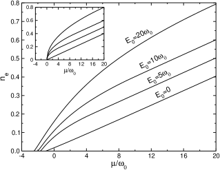
Figure 2: Electron density number $n_{e}$ as a function of the bare chemical potential $\mu$ for $\lambda=0.5$ and several values of the SO interaction $E_{0}$. The temperature is $T=0.02\omega_{0}$ and the energy cut-off is $E_{c}=100\omega_{0}$. In the inset $n_{e}$ is plotted for $\lambda=0$ and for zero temperature.

The integration over the momenta appearing in Eq.(16), or, equivalently, the integration over the energy in Eq.(19), can be carried out analytically, leaving only the summation over the Matsubara frequency to be performed numerically. Hence, for fixed values of $\lambda$, $\omega_{0}$ and $E_{0}$, the electron self-energy $\Sigma(i\omega_{n})$ is obtained by iteration of Eqs.(14), (15), and (16), while Eq.(17) is used to extract the corresponding electron density for a given value of $\mu$. For all cases we have set $E_{c}=100\omega_{0}$ and $T=0.02\omega_{0}$, which is low enough to be representative of the zero temperature case. In Fig. 2 we report the calculated values of $n_{e}$, Eq.(18), for $\lambda=0.5$ and for different values of the SO energy $E_{0}$. For comparison, we report in the inset of Fig. 2 the corresponding density values for $\lambda=0$ and at zero temperature. For $E_{0}=0$, $n_{e}$ decreases almost linearly as $\mu$ is reduced, as expected for a constant DOS in 2D (see inset), but the zero density limit $n_{e}=0$ (extracted in the $T\rightarrow 0$ limit) is reached only for $\mu=\mu_{0}\simeq-1.023\omega_{0}$, which is lower than the non-interacting zero-density value $\mu=0$. This energy decrease represents the ground state energy of a single electron in interaction with phonons and provides a measure of the strength of the el-ph interaction. For non-zero SO coupling, $E_{0}>0$, two features are apparent in Fig. 2. First, in the low density limit, $n_{e}$ is no longer a linear function of $\mu$ and, second, the ground state energy $\mu_{0}$ is even more lowered with respect to the $E_{0}=0$ case. This latter feature indicates that, for fixed $\lambda$, a single electron is more strongly coupled to phonons as $E_{0}$ increases.

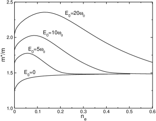
Figure 3: Electron effective mass $m^{*}$ as a function of the electron density number $n_{e}$ for $\lambda=0.5$ and for several values of the SO interaction $E_{0}$.

A more quantitative estimation of the role of SO coupling on the el-ph properties is given by the electron effective mass enhancement $m^{*}/m$. This quantity can be evaluated from

$$\frac{m^{*}}{m}=1-\frac{{\rm Im}\Sigma(i\omega_{n})}{\omega_{n}}|_{n=0}$$ (21)

provided sufficiently low temperatures are considered. We have checked that for $T=0.02\omega_{0}$ the effective mass ratio extracted from Eq. (21) is in very good accord with the mass enhancement obtained from the real frequency self-energy (see next section). In Fig. 3 we report our results for $m^{*}/m$ as a function of the electron number density $n_{e}$ for the same parameter values of Fig. 2. For $E_{0}=0$ we obtain the typical trend for a 2D electron gas in the non-crossing approximation: $m^{*}/m$ is almost a constant and approximately equal to the Migdal-Eliashberg result $1+\lambda$ for relatively large densities while, for $n_{e}\rightarrow 0$, $m^{*}/m$ decreases towards the one electron result.ccgp For $E_{0}=5\omega_{0}$, the mass enhancement follows the $E_{0}=0$ case for densities larger than $n_{e}\simeq 0.2$, corresponding to the range of densities for which $n_{e}$ is proportional to $\mu$ (see Fig. 2). Instead, for lower values of $n_{e}$, $m^{*}/m$ increases up to a maximum and eventually decreases again as $n_{e}\rightarrow 0$. Higher values of $E_{0}$ emphasize the same trend, with higher and broader maxima of $m^{*}/m$ as $E_{0}$ increases.

The results plotted in Fig. 3 clearly show how the underlying diverging DOS, Eq.(20), for $E_{0}\neq 0$ is responsible for the enhancement of the effective mass. By reading off from Fig. 2 the values of $\mu$ corresponding to the density values for which $m^{*}/m$ deviates from $1+\lambda$, it is easy to realize that the enhancement of $m^{*}/m$ starts when $\mu$ becomes lower than $\sim E_{0}$, that is when the (bare) DOS diverges as $\sqrt{E_{0}/E}$. In this situation, the coupling to the phonons is no longer parametrized by $\lambda$ alone, but rather by an effective coupling which takes into account the strongly varying DOS at low energies.ciuchi1 As a matter of fact, for small $\lambda$, by enhancing $E_{0}$ the system crosses over from a weak to a strong coupling regime, where the mass enhancement can be considerably larger than unity. It becomes therefore natural to consider signatures of such SO induced strong el-ph coupling regime also in the spectral properties of the electrons, which can provide valuable information testable by tunneling and/or photoemission experiments.gayone ; hofmann ; kroger

IV spectral properties

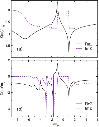
Figure 4: (color online). Real and imaginary parts of the electron self-energy for $\lambda=0.5$ and electron density $n_{e}=0.1$. The SO energy is $E_{0}=0$ in (a) and $E_{0}=5\omega_{0}$ in (b).

The self-energy for real frequencies could be obtained directly from analytical continuation on the real axis of Eqs. (14), (15) and (16). However, since convergence is faster on the imaginary axis, in this paper we opt for the more efficient method of analytical continuation formulated in Ref.[msc, ]. Hence, once $\Sigma(i\omega_{n})$ has been determined from the imaginary axis equations (14)-(16), the retarded self-energy $\Sigma_{R}(\omega)=\Sigma(\omega+i\delta)$ follows from

$$\Sigma_{R}(\omega) = -T\lambda\sum_{m}D(\omega-i\omega_{m})g(i\omega_{m})$$

$$+\lambda\frac{\omega_{0}}{2}[n(\omega_{0})+f(\omega_{0}-\omega)]g_{R}(\omega-\omega_{0})$$

$$+\lambda\frac{\omega_{0}}{2}[n(\omega_{0})+f(\omega_{0}+\omega)]g_{R}(\omega+\omega_{0}),$$

where $g_{R}(\omega\pm\omega_{0})=g(\omega\pm\omega_{0}+i\delta)$ and $n(x)$ and $f(x)$ are the distribution functions for bosons and fermions, respectively. The real and imaginary parts of $\Sigma_{R}(\omega)$ are plotted in Fig. 4 for $\lambda=0.5$, $n_{e}=0.1$, $E_{0}=0$ [Fig. 4(a)], and $E_{0}=5\omega_{0}$ [Fig. 4(b)]. The mass enhancement extracted from $m^{*}/m=\lim_{\omega\rightarrow 0}[1-d{\rm Re}\Sigma_{R}(\omega)/d\omega]$ is $1.45$ for $E_{0}=0$ and $1.72$ for $E_{0}=5\omega_{0}$, which agree with the $m^{*}/m$ values plotted in Fig. 3. For $E_{0}=0$, the self-energy displays features typical of the Holstein model for a 2D system in the non-crossing approximation. Namely, ${\rm Im}\Sigma_{R}(\omega)=0$ for $|\omega|<\omega_{0}$, while at larger frequencies ${\rm Im}\Sigma_{R}(\omega)\simeq-\pi\lambda\omega_{0}/2$. The rapid decrease of $|{\rm Im}\Sigma_{R}(\omega)|$ at negative frequencies stems from the bottom band edge. For $E_{0}=5\omega_{0}$ [Fig. 4(b)] the structure of $\Sigma_{R}(\omega)$ is more intricate due to the strong energy dependence of the underlying bare DOS. In fact, for $n_{e}=0.1$, the value of the (bare) chemical potential $\mu$ is well below $E_{0}=5\omega_{0}$ (see Fig. 2), and the $\omega$-dependence of $\Sigma_{R}(\omega)$ becomes strongly influenced by the square-root divergence of the DOS. This is particularly clear in Fig. 4(b), where ${\rm Im}\Sigma(\omega)$ reproduces for $\omega<0$ the low-energy profile of the DOS shifted by multiples of $\omega_{0}$. This feature is characteristic of a strongly-coupled el-ph system and is fully consistent with the high value of the mass enhancement ($m^{*}/m\simeq 1.72$) for this particular case.

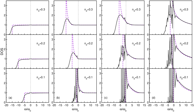
Figure 5: (color online). Reduced DOS for $\lambda=0.5$ (solid lines) and $\lambda=0$ (dashed lines). The vertical dotted line at $\omega=0$ indicates the Fermi level. The cutoff energy is $E_{c}=100\omega_{0}$ and the temperature is $T=0.02\omega_{0}$ for the interacting cases ($T=0$ for $\lambda=0$). (a): $E_{0}=0$, (b): $E_{0}=5\omega_{0}$, (c): $E_{0}=10\omega_{0}$, (d): $E_{0}=20\omega_{0}$.

A global view of the behavior for several values of the electron number density and of the SO energy is given in Fig. 5 where the reduced DOS for the interacting system

$$\rho(\omega)=-\frac{1}{\pi}{\rm Im}g_{R}(\omega)$$ (23)

is plotted for fixed $\lambda=0.5$. For comparison, we report also the bare DOS $\rho_{0}(\omega)$, Eq.(20), for the corresponding values of $n_{e}$ and $E_{0}$. For $E_{0}=0$, Fig. 5(a), reducing the electron density merely shifts the Fermi level for the interacting electron (vertical dotted line) towards the bottom of the band. For $|\omega|<\omega_{0}$ $\rho(\omega)$ coincides with the bare reduced DOS $\rho_{0}(\omega)=1$ because, as also shown in Fig. 4, the imaginary part of the self-energy is zero in that frequency range. Compared to the $\lambda=0$ case, whose DOS has a finite step at the bottom of the band, the profile of $\rho(\omega)$ is smeared by the el-ph interaction. A similar feature is obtained also for $E_{0}=5\omega_{0}$ [Fig. 5(b)] and $n_{e}=0.3$ where, now, the square-root divergence of $\rho_{0}(\omega)$ is rounded-off in $\rho(\omega)$ due to the finite lifetime for $\lambda=0.5$. However, contrary to the $E_{0}=0$ case, reducing $n_{e}$ does not translate to a (more or less) rigid shift of the Fermi level but, rather, creates new structures whose intensity increases as the Fermi level moves deeper into the square-root singularity of $\rho_{0}(\omega)$. This is even more pronounced for $E_{0}=10\omega_{0}$ and $E_{0}=20\omega_{0}$ plotted respectively in Figs. 5 (c) and (d). For the latter cases, the profile of $\rho(\omega)$ for $n_{e}=0.1$ is characterized by well defined peaks separated by multiples of $\omega_{0}$, and whose widths decrease as $E_{0}/\omega_{0}$ is enhanced.

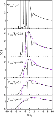
Figure 6: (color online). Reduced DOS for $\lambda=0.5$ (solid lines) and $\lambda=0$ (dashed lines) for several values of the impurity scattering rate $\Gamma_{\rm imp}$. The temperature is $T=0.02\omega_{0}$ and $E_{0}=10\omega_{0}$, $n_{e}=0.1$ for all cases.

Such strong-coupling features are in principle directly observable by means of low-temperature tunneling or photoemission measurements provided, however, that other interactions do not alter significantly the profile of $\rho(\omega)$. This could be not the case for example when disorder effects are taken into account, since these tend to smear all sharp features of the DOS even at zero temperature. To investigate this point, we have considered a coupling to a short-range impurity potential of the form $V({\bf r})=V_{\rm imp}\sum_{i}\delta({\bf r}-{\bf R}_{i})$, where ${\bf R}_{i}$ are the random positions of impurity scatterers. Within the self-consistent Born approximation, the resulting self-energy is hence given by Eq.(15) with the impurity term $\Gamma_{\rm imp}g(i\omega_{n})/\pi$ added in the right-hand side, and Eq.(IV) modified accordingly. The parameter $\Gamma_{\rm imp}=1/2\tau_{\rm imp}=\pi n_{i}V_{\rm imp}^{2}N_{0}$ is the usual scattering rate for zero SO coupling and for density $n_{i}$ of impurities. In Fig. 6 we report the calculated reduced DOS $\rho(\omega)$ for $\lambda=0.5$, $E_{0}=10\omega_{0}$, $n_{e}=0.1$ and for several values of $\Gamma_{\rm imp}$. Also plotted by dashed lines for $\Gamma_{\rm imp}\neq 0$ are the corresponding DOS curves in the absence of el-ph interaction ($\lambda=0$). Compared to the clean limit $\Gamma_{\rm imp}=0$ (top panel), for rather weak disorder ($\Gamma_{\rm imp}=0.02E_{0}$) the phonon peaks at $\omega<0$ are considerably less sharp and slighly shifted at more negative frequencies, but nevertheless still clearly discernible. Larger values of $\Gamma_{\rm imp}$ increasingly smear the phonon structures, and gradually the peaks disappear. For $\Gamma_{\rm imp}=0.2E_{0}$ (which corresponds to $\Gamma_{\rm imp}=2\omega_{0}$) the resulting DOS is basically dominated by the impurity interaction, and does not deviate much from the $\lambda=0$ case.

V discussion

In this section we review the meaning of the approximations used in the present work and discuss alternative models for the study of the el-ph interaction in strong Rashba SO systems. Let us start by considering the limitations of the non-crossing approximation for the electron self-energy. For zero SO interaction, or for Fermi energies sufficiently larger than $E_{0}$, this is a rather good description of the el-ph problem provided $\lambda$ is sufficiently small. However, as we have seen, for non-zero SO interaction the electrons behave as effectively strongly coupled to the phonons when the Fermi level is below $E_{0}$. This is because of the square-root singularity in the DOS when $E_{0}\neq 0$. In the $E_{F}<E_{0}$ regime, therefore, the non-crossing approximation, although making evident the trend towards strong coupling, may not be adequate for a more trustworthy description of the system. It is instructive at this point to consider the limiting situation where only one electron is present. By using second-order perturbation theory (that is simply the non-crossing approximation with the bare electron Green’s function) it is easy to evaluate the mass enhancement factor. At zero temperature, and setting for simplicity $E_{c}/E_{0}=\infty$, this is given by

$$\frac{m^{*}}{m}=1+\frac{\lambda}{2}+\frac{\lambda}{2}\sqrt{\frac{E_{0}}{\omega_{0}}}\arctan\!\left(\sqrt{\frac{E_{0}}{\omega_{0}}}\right).$$ (24)

It is clear from the above expression that for $E_{0}\gg\omega_{0}$ the mass enhancement factor is governed by an effective coupling, say $\tilde{\lambda}$, proportional to $\lambda\sqrt{E_{0}/\omega_{0}}$, amplified with respect to $\lambda$ by the square-root divergent DOS. Equation (24) clarifies also that the relevant adiabatic parameter for $E_{F}\ll E_{0}$ is $\omega_{0}/E_{0}$, rather than $\omega_{0}/E_{c}$ (where $E_{c}$ plays the role of the bandwidth), and that the effective coupling $\tilde{\lambda}$ increases as $\omega_{0}/E_{0}\rightarrow 0$. Consequently, in the adiabatic limit $\omega_{0}/E_{0}=0$ perturbation theory breaks down for any finite $\lambda$ because $\tilde{\lambda}=\infty$. This leads us to suspect that, in analogy with the adiabatic limit of the one-dimensional lattice Holstein model,kabanov the ground state of a single electron for $\omega_{0}/E_{0}=0$ is always a bound polaron. However, for $\omega_{0}/E_{0}\neq 0$, the effective coupling $\tilde{\lambda}\simeq\lambda\sqrt{E_{0}/\omega_{0}}$ is finite, which permits to estimate a rough range of validity of Eq.(24). Indeed, contributions of higher orders of perturbation theory become negligible as long as $\tilde{\lambda}\ll 1$, corresponding to $\lambda\ll\sqrt{\omega_{0}/E_{0}}$, consistent with the results on the one-dimensional Holstein model of Refs.[marsiglio, ; ccg, ], which show better agreement between perturbation theory and exact diagonalization results as $\omega_{0}$ increases.

Also for low but finite electron densities it is possible to interpret the coupling to the phonons in terms of an effective el-ph coupling $\tilde{\lambda}$ which grows as $E_{0}$ increases. For example, in the range of electron densities $n_{e}=0.1$-$0.2$, the mass enhancement factor plotted in Fig. 3 for $\lambda=0.5$ may be interpreted by an effective Migdal-Eliashberg formula $m^{*}/m=1+\tilde{\lambda}$, where $\tilde{\lambda}\approx 1$ for $E_{0}=10\omega_{0}$ and $\tilde{\lambda}\approx 1.3$ for $E_{0}=20\omega_{0}$. However, contrary to the one-electron case discussed above, now $\tilde{\lambda}$ depends on the Fermi energy $E_{F}$. Indeed, provided that $\omega_{0}<E_{F}<E_{0}$, the effective coupling turns out to be of order $\tilde{\lambda}\simeq\lambda\sqrt{E_{0}/E_{F}}$, where the square-root term stems from the singularity of the DOS, Eq.(20), in analogy with the general definition of the effective el-ph interaction in the presence of a van Hove singularity.cappelluti At this point it is possible to estimate the validity of the self-consistent non-crossing approximation for the self-energy considered in the previous sections. In fact, according to Migdal’s theorem generalized to systems with diverging DOS,cappelluti the el-ph vertex correction factors beyond the non-crossing approximation are at least of order $P=\tilde{\lambda}\omega_{0}/E_{F}$, so that neglecting them would introduce an error of order $P$. Estimates of $P$ for the different cases discussed in this paper can be obtained by evaluating $\tilde{\lambda}\simeq 1-m^{*}/m$ from Fig.3. In this way the Fermi energy is roughly given by $E_{F}\simeq(\lambda/\tilde{\lambda})^{2}E_{0}$, which then can be inserted in the definition of $P$. For the low density value $n_{e}=0.1$ we find $P\gtrsim 1$ for $E_{0}=20\omega_{0}$ and $P\simeq 0.5$ for $E_{0}=10\omega_{0}$, showing that the non-crossing approximation is quantitatively inaccurate in this case. However, already for $n_{e}=0.2$, for which effectively strong-coupling features are apparent from Fig.3 and Fig.4, the contributions of the vertex corrections drop to $P\simeq 0.4$ and $P\simeq 0.2$ for $E_{0}=20\omega_{0}$ and $E_{0}=10\omega_{0}$, respectively. In this situation, the non-crossing approximation is fairly reliable and its accuracy improves as $n_{e}$ is further enhanced and/or $E_{0}/\omega_{0}$ is reduced.

Let us turn now to discuss the general form of the self-energy for the case in which the el-ph matrix element is momentum dependent. Here we consider the situation in which the momentum dependence is only through the modulus $q$ of the momentum transfer ${\bf q}$, as is the case, for example, with the 2D Fröhlich model, for which the coupling goes like $1/\sqrt{q}$. As shown in the Appendix, a fully general expression of the self-energy valid also beyond the non-crossing approximation is:

$$\mathbf{\Sigma}({\bf k},i\omega_{n})=\Sigma_{1}(k,i\omega_{n})\mathbf{1}+\Sigma_{2}(k,i\omega_{n})\hat{\mathbf{\Omega}}_{\bf k}\cdot\mbox{\boldmath$\sigma$},$$ (25)

where $\Sigma_{1}$ and $\Sigma_{2}$ are scalars. Compared to Eq.(15), the above expression has an additional term which is off-diagonal in the spin subspace, renormalizing therefore the SO coupling. This term disappears ($\Sigma_{2}=0$) only when the el-ph matrix element is momentum independent, like in the Holstein model, and at the same time the self-energy is evaluated in the non-crossing approximation. In all other cases, like, e.g., the Fröhlich model in the non-crossing approximation, $\Sigma_{2}$ is nonzero. For sufficiently large values of $E_{F},$ such that the weak SO limit $E_{0}/E_{F}\ll 1$ holds true so that the Fermi level lies far above the 1D singularity of the DOS, $\Sigma_{2}$ turns out to be of order $\lambda\omega\Delta_{\rm so}/E_{F}\propto\lambda\omega_{0}\sqrt{E_{0}/E_{F}}$, and can be disregarded in comparison with $\Sigma_{1}\approx\lambda\omega_{0}$. On the contrary, when $E_{F}/E_{0}\lesssim 1$, $\Sigma_{1}$ and $\Sigma_{2}$ have comparable magnitude, and the full momentum and frequency dependent of both terms must be considered for a consistent evaluation of the el-ph effects.

VI conclusions

In this paper we have addressed the role of the Rashba SO interaction in the properties of a coupled el-ph gas in two dimensions. By using a self-consistent non-crossing approximation for the electron self-energy, we have studied the mass enhancement factor and the spectral properties. We have shown that, for sufficiently strong SO interaction, the electron becomes strongly coupled to the phonons even if el-ph coupling $\lambda$ can be classified as weak. We identify this behavior as being due to a topological change of the Fermi surface for strong SO interaction, which gives rise to a square-root singularity in the DOS at low energies. Signatures of such effectively strong el-ph coupling are found in the mass enhancement factor, which becomes as large as $m^{*}/m\approx 2$ for el-ph coupling of only $\lambda=0.5$, and in the energy dependence of the interacting DOS, displaying low energy peaks separated by multiples of the phonon energy $\omega_{0}$. This latter feature could be tested experimentally by tunneling or photoemission experiments in systems where the Fermi level can be tuned to approach the square-root singularity of the DOS. We have then discussed limitations of the non-crossing approximation approach and possible generalizations of the theory for momentum-dependent el-ph matrix elements. Since the problem of el-ph coupling in the presence of SO interaction is relevant for several systems such as metal and semimetal surface states, surface superconductors, or low-dimensional heterostructures, and given the current interest in spintronic physics, we hope that our work will stimulate further investigations.

*

Appendix A

In this appendix we evaluate the form of the electron self-energy when the el-ph interaction is momentum dependent. In particular, we consider the hamiltonian $H=H_{0}+H_{ph}$, where $H_{0}$ is the Rashba spin-orbit hamiltonian of Eq.(1) and

$$H_{ph}=\sum_{\bf q}\omega_{0}a^{\dagger}_{\bf q}a_{\bf q}+\sum_{\mathbf{k}\mathbf{k}^{\prime}\alpha}g_{{\bf k}-{\bf k}^{\prime}}c^{\dagger}_{\mathbf{k}\alpha}c_{\mathbf{k}^{\prime}\alpha}(a^{\dagger}_{\mathbf{k}-\mathbf{k}^{\prime}}+a_{\mathbf{k}^{\prime}-\mathbf{k}}),$$ (26)

where $g_{\bf q}$ is the el-ph matrix element which we assume depends only on the modulus of momentum transfer ${\bf q}$. It is convenient to rewrite $H$ in terms of the eigenvectors of $H_{0}$, whose annihilation operators $d_{{\bf k}s}$ ($s=\pm$) are related to $c_{{\bf k}\alpha}$ through

$$\left(\begin{array}[]{c}d_{{\bf k}+}\\ d_{{\bf k}-}\end{array}\right)=\mathbf{T}_{\bf k}\left(\begin{array}[]{c}c_{{\bf k}\uparrow}\\ c_{{\bf k}\downarrow}\end{array}\right)=\frac{1}{\sqrt{2}}\left(\begin{array}[]{cc}1&-ie^{-i\varphi}\\ 1&ie^{-i\varphi}\end{array}\right)\left(\begin{array}[]{c}c_{{\bf k}\uparrow}\\ c_{{\bf k}\downarrow}\end{array}\right),$$ (27)

where $\varphi$ is the azimuthal angle of ${\bf k}$. In this basis, $H_{0}$ is diagonal with dispersion relation given by Eq.(3) while $H_{ph}$ becomes

$$H_{ph}=\sum_{\bf q}\omega_{0}a^{\dagger}_{\bf q}a_{\bf q}+\sum_{\mathbf{k}\mathbf{k}^{\prime}ss^{\prime}}M^{s,s^{\prime}}_{{\bf k}-{\bf k}^{\prime}}d^{\dagger}_{\mathbf{k}s}d_{\mathbf{k}^{\prime}s^{\prime}}(a^{\dagger}_{\mathbf{k}-\mathbf{k}^{\prime}}+a_{\mathbf{k}^{\prime}-\mathbf{k}}),$$ (28)

with

$$M^{s,s^{\prime}}_{{\bf k}-{\bf k}^{\prime}}=g_{{\bf k}-{\bf k}^{\prime}}\frac{1+ss^{\prime}e^{i(\varphi-\varphi^{\prime})}}{2}.$$ (29)

By applying Wick’s theorem, it turns out that, to all orders of the el-ph interaction, the Green’s function in the chiral basis has zero off-diagonal components so that, if $G_{\pm}({\bf k},\tau)=-\langle T_{\tau}d_{{\bf k}\pm}(\tau)d^{\dagger}_{{\bf k}\pm}(0)\rangle$, the matrix Green’s function in the original spin sub-space becomes

$$\mathbf{G}({\bf k},i\omega_{n}) =\mathbf{T}^{\dagger}_{\bf k}\left(\begin{array}[]{cc}G_{+}({\bf k},i\omega_{n})&0\\ 0&G_{-}({\bf k},i\omega_{n})\end{array}\right)\mathbf{T}_{\bf k}$$ (32)

$$=\frac{1}{2}\sum_{s=\pm}(1+s\hat{\mathbf{\Omega}}_{\bf k}\cdot\mbox{\boldmath$\sigma$})G_{s}({\bf k},i\omega_{n}).$$ (33)

Consequently, by using Dyson’s equation (9), the matrix self-energy in the spin sub-space is

$$\mathbf{\Sigma}({\bf k},i\omega_{n})=\Sigma_{1}({\bf k},i\omega_{n})\mathbf{1}+\Sigma_{2}({\bf k},i\omega_{n})\hat{\mathbf{\Omega}}_{\bf k}\cdot\mbox{\boldmath$\sigma$},$$ (34)

where

$$\Sigma_{1(2)}({\bf k},i\omega_{n})=\frac{\Sigma_{+}({\bf k},i\omega_{n})+(-)\Sigma_{-}({\bf k},i\omega_{n})}{2}.$$ (35)

In order to obtain Eq.(25), it suffices to demonstrate that the momentum dependence of self-energy in the chiral basis, $\Sigma_{\pm}({\bf k},i\omega_{n})$, is only via $k=|{\bf k}|$. This is accomplished by noticing that the el-ph matrix element in the chiral basis, Eq.(29), depends on the direction of the momentum transfer ${\bf k}-{\bf k}^{\prime}$ solely through $\varphi-\varphi^{\prime}$. Hence, if the electronic dispersion depends only on the modulus of the momentum, as is the case with Eq.(3), a general self-energy diagram in the chiral basis will be independent of the direction of ${\bf k}$ which, by using (35), is consistent with Eq.(25).

References

- (1) G. Prinz, Phys. Today 48 (4), 58 (1995).
- (2) I. Žutić, J. Fabian, and S. Das Sarma, Rev. Mod. Phys. 76, 323 (2004).
- (3) E. I. Rashba, Sov. Phys. Solid State 2, 1224 (1960).
- (4) G. Dresselhaus, Phys. Rev. 100, 580 (1955).
- (5) X. C. Zhang, A. Pfeuffer-Jeschke, K. Ortner, V. Hock, H. Buhmann, C. R. Becker, and G. Landwehr, Phys. Rev. B 63, 245305 (2001).
- (6) Y. S. Gui, C.R. Becker, N. Dai, J. Liu, Z.J. Qiu, E.G. Novik, M. Schafer, X.Z. Shu, J.H. Chu, H. Buhmann, and L.W. Molenkamp, Phys. Rev. B 70, 115328 (2004)
- (7) S. LaShell, B. A. McDougall, and E. Jensen, Phys. Rev. Lett. 77, 3419 (1996).
- (8) Yu. M. Koroteev, G. Bihlmayer, J. E. Gayone, E. V. Chulkov, S. Blugel, P. M. Echenique, and P. Hofmann, Phys. Rev. Lett. 93, 046403 (2004).
- (9) K. Sugawara, T. Sato, S. Souma, T. Takahashi, M. Arai, and T. Sasaki, Phys. Rev. Lett. 96, 046411 (2006).
- (10) J. R. McLaughlan, E. M. Llewellyn-Samuel, and S. Crampin, J. Phys.: Condens. Matter 16, 6841 (2004).
- (11) E. Rotenberg, J. W. Chung, and S. D. Kevan, Phys. Rev. Lett. 82, 4066 (1999).
- (12) D. Pacilé, C. R. Ast, M. Papagno, C. Da Silva, L. Moreschini, M. Falub, A. P. Seitsonen, and M. Grioni, Phys. Rev. B 73 245429 (2006).
- (13) C. R. Ast, G. Wittich, P. Wahl, R. Vogelgesang, D. Pacilé, M. C. Falub, L. Moreschini, M. Papagno, M. Grioni, and K. Kern, Phys. Rev. B 75, 201401(R) (2007).
- (14) C. R. Ast, J. Henk, A. Ernst, L. Moreschini, M. C. Falub, D. Pacilé, P. Bruno, K. Kern, and M. Grioni, Phys. Rev. Lett. 98, 186807 (2007).
- (15) I. Barke, F. Zheng, T. K. Rügheimer, and F. J. Himpsel, Phys. Rev. Lett. 97, 226405 (2006).
- (16) E. Bauer, G. Hilscher, H. Michor, C. Paul, E. W. Scheidt, A. Gribanov, Y. Seropegin, H. Noel, M. Sigrist, and P. Rogl, Phys. Rev. Lett. 92, 027003 (2004).
- (17) K. V. Samokhin, E. S. Zijlstra, and S. K. Bose, Phys. Rev. B 69, 094514 (2004).
- (18) K. Togano, P. Badica, Y. Nakamori, S. Orimo, H. Takeya, and K. Hirata, Phys. Rev. Lett. 93, 247004 (2004).
- (19) H. Q. Yuan, D. F. Agterberg, N. Hayashi, P. Badica, D. Vandervelde, K. Togano, M. Sigrist, and M. B. Salamon, Phys. Rev. Lett. 97, 017006 (2006).
- (20) C. R. Ast, D. Pacilé, M. Falub, L. Moreschini, M. Papagno, G. Wittich, P. Wahl, R. Vogelgesang, M. Grioni, K. Kern, cond-mat/0509509 (2005).
- (21) A. V. Chaplik and L. I. Magarill, Phys. Rev. Lett. 96, 126402 (2006).
- (22) E. Cappelluti, C. Grimaldi, and F. Marsiglio, Phys. Rev. Lett. 98, 167002 (2007).
- (23) J. E. Gayone, S. V. Hoffmann, Z. Li, and Ph. Hofmann, Phys. Rev. Lett. 91, 127601 (2003).
- (24) Ph. Hofmann, Prog. Surf. Sci. 81, 191 (2006).
- (25) S. LaShell, B. A. McDougall, and E. Jensen, Phys. Rev. B 74, 033410 (2006).
- (26) J. Kröger, Rep. Prog. Phys. 69, 899 (2006).
- (27) L. P. Gor’kov, Int. J. Mod. Phys. B 20, 2569 (2006).
- (28) A. A. Abrikosov, L. P. Gorkov, and I. E. Dzyaloshinsky, Methods of Quantum Field hoery in statistical Physics, (Dover, New York, 1975).
- (29) E. Cappelluti, S. Ciuchi, C. Grimaldi, and L. Pietronero, Phys. Rev. B 68, 174509 (2003).
- (30) S. Ciuchi, F. de Pasquale, S. Fratini, and D. Feinberg, Phys. Rev. B 56, 4494 (1997).
- (31) F. Marsiglio, M. Schossmann, and J. P. Carbotte, Phys. Rev. B 37, 4965 (1988).
- (32) V. V. Kabanov and O. Yu. Mashtakov, Phys. Rev. B 47, 6060 (1993). See also discussion in Ref.[ciuchi1, ].
- (33) F. Marsiglio, Phys. LEtt. A 180, 280 (1993).
- (34) M. Capone, S. Ciuchi, and C. Grimaldi, Europhys. Lett. 42, 523 (1998).
- (35) E. Cappelluti and L. Pietronero, Phys. Rev. B 53, 932 (1996).