ELECTRONIC STRUCTURE OF SPHEROIDAL FULLERENES

RICHARD PINCAK^a,b and MICHAL PUDLAK^a

^aInstitute of Experimental Physics, Slovak Academy of Sciences,

Watsonova 47,043 53 Kosice, Slovak Republic

^bBogoliubov Laboratory of Theoretical Physics,

Joint Institute for Nuclear Research, Dubna, Russia

Abstract

Both the eigenfunctions and the local density of states (DOS) near the pentagonal defects on the fullerenes was calculated analytically as a numerically. The results shows that the low-energy DOS has a cusp which drops to zero at the Fermi energy for any number of pentagons at the tip except three. For three pentagons, the nonzero DOS across the Fermi level is formed. Graphite is an example of a layered material that can be bent to form fullerenes which promise important applications in electronic nanodevices. The spheroidal geometry of a slightly elliptically deformed sphere was used as a possible approach to fullerenes. We assumed that for a small deformation the eccentricity of the spheroid is much more smaller then one. We are interested in the elliptically deformed fullerenes C₇₀ as well as in C₆₀ and its spherical generalizations like big C₂₄₀ and C₅₄₀ molecules. The low-lying electronic levels are described by the Dirac equation in (2+1) dimensions. We show how a small deformation of spherical geometry evokes a shift of the electronic spectra compared to the sphere and both the electronic spectrum of spherical and the shift of spheroidal fullerenes were derived. In the next study the expanded field-theory model was proposed to study the electronic states near the Fermi energy in spheroidal fullerenes. The low energy electronic wave functions obey a two-dimensional Dirac equation on a spheroid with two kinds of gauge fluxes taken into account. The first one is so-called K spin flux which describes the exchange of two different Dirac spinors in the presence of a conical singularity. The second flux (included in a form of the Dirac monopole field) is a variant of the effective field approximation for elastic flow due to twelve disclination defects through the surface of a spheroid. We consider the case of a slightly elliptically deformed sphere which allows us to apply the perturbation scheme. We shown exactly how a small deformation of spherical fullerenes provokes an appearance of fine structure in the electronic energy spectrum as compared to the spherical case. In particular, two quasi-zero modes in addition to the true zero mode are predicted to emerge in spheroidal fullerenes. The effect of a weak uniform magnetic field on the electronic structure of slightly deformed fullerene molecules was also studied. It was shown how the existing due to spheroidal deformation fine structure of the electronic energy spectrum splitted in the presence of the magnetic field. We shown that the fine structure of the electronic energy spectrum is very sensitive to the orientation of the magnetic field. We found that the magnetic field pointed in the x direction does not influence the first electronic level whereas it causes a splitting of the second energy level. Exact analytical solutions for zero-energy modes are found. The HOMO (highest occupied molecular orbital)-LUMO (lowest unoccupied molecular orbital) gap was calculated within the continuum field-theory model of fullerenes.

Chapter 1 Introduction

The purpose of this chapter is to present some examples of using topology and geometry in a study of a new interesting class of carbon materials as fullerenes. Fullerenes are cage-like molecules of carbon atoms. The discovery of these molecules has attracted considerable attention of both experimentalists and theorists due to their unique physical properties. An further interest to carbon nanoparticles originates from the fact that the geometry is accompanied by topological defects. The topologically nontrivial objects play the important role in various physically interesting systems. The ’t Hooft-Polyakov monopole in the non-Abelian Higgs model, instantons in quantum chromodynamics, solitons in the Skyrme model, Nielsen-Olesen magnetic vortices in the Abelian Higgs model(see, e.g., [1]) are examples of such topologically nontrivial objects. Notice that the topological origin the elastic flux results in appearance of the disclination-induced Aharanov-Bohm like phase (see [2]). In condensed matter physics for instance, vortices in liquids and liquid crystals, solitons in low-dimensional systems are objects with nontrivial topology.

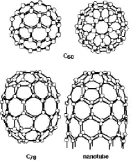
Figure 1.1: The symmetric structure of fullerene C₆₀, elliptically deformed molecule C₇₈ and big deformed structure as carbon nanotube.

The high flexibility of carbon allows producing variously shaped carbon nanostructures: fullerenes, nanotubes, nanohorns, cones, toroids, graphitic onions, etc. Some of them as e.g.nanotubes are composition of tubes and fullerenes (as in Fig. 1.1).Historically, the fullerenes C₆₀ (nicknamed also as Buckminsterfullerene or ’bucky ball’) were first discovered in 1985 [3]. They are tiny molecular cages of carbon having 60 atoms and making up the mathematical shape called a truncated icosahedron (12 pentagons and 20 hexagons). The amount of C₆₀ had been produced in small quantities until 1990 when an efficient method of production was achieved [4]. Since then, there were produced variously shaped fullerene molecules. These molecules are formed when $12$ pentagons are introduced in the hexagonal lattice of graphene. Soon after the fullerenes, the carbon nanotubes of different diameters and helicity [5] were produced. We can also image the construction of nanotube with fullerenes as a cap at the end of nanotubes (see Fig. 1.2). The mechanical, magnetic, and especially electronic properties of carbon nanotubes are found to be very specific (see, e.g., [6]).

Figure 1.2: The fullerene C₆₀ and spheroidal ones as a cap at the end of some nanotubes.

The fullerenes are composed of hexagonal and pentagonal carbon rings. However, the structures having heptagonal rings are also possible. A junction which connect carbon nanotubes with different diameters through a region sandwiched by pentagon-heptagon pair has been observed in the transmission electron microscope [7]. A pair of five- and seven-membered rings have to be imposed to connect two different types of carbon nanotubes [8]. Theoretically the closed fullerenes and nanotubes exhibiting high topologies (from genus 5 to genus 21) were suggested in [9]. This follows from the known Euler’s theorem that relates the number of vertices, edges and faces of an object. For the hexagonal carbon lattice it can be written in the form [9]

$$...2n_{4}+n_{5}-n_{7}-2n_{8}...=\sum(6-x)n_{x}=\chi=12(1-g),$$ (1.1)

where $n_{x}$ is the number of polygons having $x$ sides, $\chi$ is the Euler characteristic which is a geometrical invariant related to the topology of the structure, and $g$ is the genus or a number of handles of an arrangement. According to (1.1) there is no contribution to the Gaussian curvature for $x=6$. This means that two-dimensional carbon lattice consisting only of hexagons is flat. By their nature, pentagons (as well as other polygons with $x\neq 6$) in a graphite sheet are topological defects (see Fig. 1.3).

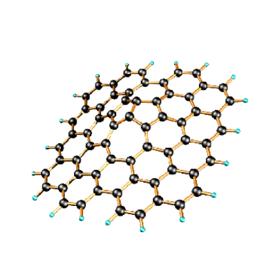
Figure 1.3: The pentagonal and heptagonal defects in the hexagonal network.

In particular, fivefold coordinated particles are orientational 60^∘ disclination defects in the sixfold coordinated triangular lattice. Description of the electronic structure requires formulating a theoretical model describing electrons on arbitrary curved surfaces with disclinations taken into account. The most important fact found in [10, 11, 12] is that the electronic spectrum of a single graphite plane linearized around the corners of the hexagonal Brillouin zone coincides with that of the Dirac equation in (2+1) dimensions. This finding stimulated a formulation of some field-theory models for Dirac fermions on hexatic surfaces to describe electronic structure of variously shaped carbon materials: fullerenes [13, 14] and nanotubes [15]. The field-theory models for Dirac fermions on a plane and on a sphere [16] were invoked to describe variously shaped carbon materials.

Chapter 2 Electronic properties

Carbon nanoparticles and their electronic properties have been a subject of an extensive study. Electronic states in nanotubes, fullerenes, nanocones, nanohorns as well as in other carbon configurations are the subject of an increasing number of experimental and theoretical studies. It has been predicted and later observed in experiment that bending or stretching a nanotube change its band structure changing therefore the electrical properties: stretched nanotubes become either more or less conductive. Carbon nanotubes can be either a metal or semiconductor, depending on their diameters and helical arrangement [17]. This finding could allow to build nanotube-based transducers sensitive to tiny forces.

The electronic properties depends on the topological defects. The peculiar electronic states due to topological defects have been observed in different kinds of carbon nanoparticles by scanning tunneling microscopy (STM). For example, STM images with five-fold symmetry (due to pentagons in the hexagonal graphitic network) have been obtained in the C₆₀ fullerene molecule [18]. The peculiar electronic properties at the ends of carbon nanotubes (which include several pentagons) have been probed experimentally in [19, 20]. Recently, the electronic structure of a single disclination has been revealed on an atomic scale by STM [21].

The problem of peculiar electronic states near the pentagons in curved graphite nanoparticles was the subject of intensive theoretical studies in fullerenes [14, 13], nanotubes [15], nanohorns [22], and cones [23]. In particular, an analysis within the effective-mass theory has shown that a specific $\sqrt{3}\times\sqrt{3}$ superstructure induced by pentagon defects can appear in nanocones [24]. This prediction has been experimentally verified in [21]. A recent study [25] within both tight-binding and ab initio calculations shows a presence of sharp resonant states in the region close to the Fermi energy. The localized cap states in nanotubes have been recently studied in [26].

It is interesting to note that the problem of specific electronic states at the Fermi level due to disclinations is similar to that of the fermion zero modes for planar systems in a magnetic field. Generally, zero modes for fermions in topologically nontrivial manifolds have been of current interest both in the field theory and condensed matter physics. As was revealed, they play a major role in getting some insight into understanding anomalies [27] and charge fractionalization that results in unconventional charge-spin relations (e.g. the paramagnetism of charged fermions) [28] with some important implications for physics of superfluid helium (see, e.g., review [29]). $3D$ space-time Dirac equation for massless fermions in the presence of the magnetic field was found to yield $N-1$ zero modes in the N-vortex background field [30]. As it was shown in [13], the problem of the local electronic structure of fullerene is closely related to Jackiw’s analysis [30]. An importance of the fermion zero modes was also discussed in the context of the high-temperature chiral superconductors [31]. Among different theoretical approaches to describe graphene compositions, the continuum model play a special role. It allow us to describe some integral features of similar carbon structures. It should be noted that the formulation of any continuum model begins from description of a graphite sheet (graphene). We briefly report now the effective mass theory for graphene [11, 12]. A single layer of graphite forms a two-dimensional material. Two Bloch functions constructed from atomic orbitals for two inequivalent carbon atoms, A and B, in the unit cell provide the basis function for graphene. The Bloch basis functions $\Phi_{j}$ ($j=A,B$) are constructed from atomic $2p_{z}$ orbitals

$$\Phi_{A}(\vec{k},\vec{r})=\sum_{n}\frac{1}{\sqrt{N}}\ e^{i\vec{k}\ \vec{r}_{n}}f(\vec{r}-\vec{r_{n}}),$$ (2.1)

$$\Phi_{B}(\vec{k},\vec{r})=\sum_{n}\frac{1}{\sqrt{N}}\ e^{i\vec{k}\ \vec{r}_{n}}f(\vec{r}-\vec{d}-\vec{r_{n}}),$$ (2.2)

$\vec{d}$ is a coordinate of $B$ atom in the unit cell, $N$ is a number of unit cell, $\vec{r}_{n}$ is a unit cell coordinate, $f$ is $2p_{z}$ orbital, $\vec{k}$ is the wave vector. Now we want to solve the Schrödinger equation

$$\hat{H}\Phi=E\Phi,$$ (2.3)

where $\Phi=c_{A}\Phi_{A}+c_{B}\Phi_{B}$ and $\hat{H}$ is the Hamiltonian of the system. We get the secular equations

$$H_{AA}c_{A}+H_{AB}C_{B}=EC_{A},$$

$$H_{BA}c_{A}+H_{BB}C_{B}=EC_{B},$$ (2.4)

here

$$H_{ij}=\langle\Phi_{i}|\hat{H}|\Phi_{j}\rangle,\quad i,j=A,B.$$ (2.5)

In a tight-binding approximation it have a form

$$\hat{H}_{AA}=\hat{H}_{BB}=\varepsilon_{2p},$$

$$\hat{H}_{AB}=t\left(e^{i\vec{k}\vec{\tau}_{1}}+e^{i\vec{k}\vec{\tau}_{2}}+e^{i\vec{k}\vec{\tau}_{3}}\right),$$ (2.6)

where $\varepsilon_{2p}$ is a orbital energy of the $2p_{z}$ level and $\vec{\tau}_{i}$ are the coordinates of the three nearest-neighbor $B$ atoms relative to an A atom

$$t=\langle f(\vec{r})|\hat{H}|f(\vec{r}-\vec{d}\ )\rangle.$$ (2.7)

Solving the secular equation

$$det\left(H-E\right)=0,$$ (2.8)

the eigenvalues $E(\hat{k})$ are obtained in the form

$$E(\vec{k})=\varepsilon_{2p}\pm t\sqrt{1+4\cos\frac{ak_{x}}{2}\cos\frac{\sqrt{3}ak_{y}}{2}+4\cos^{2}\frac{ak_{x}}{2}}.$$ (2.9)

We have

$$E(\vec{K})=E(\vec{K}^{{}^{\prime}})=\varepsilon_{2p},$$ (2.10)

and the $\vec{K}$ and $\vec{K}^{{}^{\prime}}$ points are the corners of the Brillouin zone. In $\vec{k}.\vec{p}$ theory we approximate the wave function at wave vector $\hat{k}=\hat{K}+\hat{\kappa}$ by

$$\Phi(\hat{k},\hat{r})=c_{A}(\hat{\kappa})e^{i\hat{\kappa}.\hat{r}}\Phi_{A}(\hat{K},\hat{r})+c_{B}(\hat{\kappa})e^{i\hat{\kappa}.\hat{r}}\Phi_{B}(\hat{K},\hat{r}).$$ (2.11)

Inserting $\Phi$ into Schrödinger equation, keeping terms of order $\vec{\kappa}$, we get the secular equation ($\hbar=c=1$ units are used)

$$\frac{\vec{\kappa}}{m}.\left(\begin{array}[]{cc}\vec{p}_{AA}&\vec{p}_{AB}\\ \vec{p}_{BA}&\vec{p}_{BB}\end{array}\right)\left(\begin{array}[]{c}c_{A}(\vec{\kappa})\\ c_{B}(\vec{\kappa})\end{array}\right)=E(\vec{\kappa})\left(\begin{array}[]{c}c_{A}(\vec{\kappa})\\ c_{B}(\vec{\kappa})\end{array}\right),$$ (2.12)

where $E(\vec{\kappa})=E(\vec{k})-E(\vec{K})$ and

$$\vec{p}_{ij}=\int\Phi_{i}^{*}(\hat{K},\hat{r})\vec{p}\Phi_{j}(\hat{K},\hat{r})d\vec{r}\ i,j=A,B.$$ (2.13)

It can be shown from group theoretical argument (and can be verify directly within the one-orbital tight-binding model) that the secular equation can be write in the form [12, 10]

$$v_{F}\left(\begin{array}[]{cc}0&\kappa_{x}-i\kappa_{y}\\ \kappa_{x}+i\kappa_{y}&0\end{array}\right)\left(\begin{array}[]{c}c_{A}(\vec{\kappa})\\ c_{B}(\vec{\kappa})\end{array}\right)=E(\vec{\kappa})\left(\begin{array}[]{c}c_{A}(\vec{\kappa})\\ c_{B}(\vec{\kappa})\end{array}\right),$$ (2.14)

where $v_{F}=\frac{\sqrt{3}at}{2}$, $a$ is the lattice constant and

$$E(\vec{\kappa})=\pm v_{F}|\vec{\kappa}|.$$ (2.15)

The upper half of the energy dispersion curves describes the $\pi^{*}$-energy anti-bonding band, and the lower half is the $\pi$ energy bonding band. Since there are two $\pi$ electrons per unit cell, the lower $\pi$ band is fully occupied. The points $K$,$K^{{}^{\prime}}$ create the Fermi surface of the graphene. When an external gauge fields are imposed, the translation symmetry can be broken and eigenfunction can no longer be labeled by $\vec{\kappa}$. This requires a generalization of the trial wave function

$$\Phi(\hat{r})=\int c_{A}(\hat{\kappa})e^{i\hat{\kappa}.\hat{r}}\Phi_{A}(\hat{K},\hat{r})d\vec{\kappa}+\int c_{B}(\hat{\kappa})e^{i\hat{\kappa}.\hat{r}}\Phi_{B}(\hat{K},\hat{r})d\vec{\kappa}.$$ (2.16)

Inserting this function into Schrödinger equation leads to an equation [10, 32]

$$\left(-iv_{F}\vec{\sigma}.(\vec{\nabla}-i\vec{W})-E\right)\left(\begin{array}[]{c}\Psi_{A}(\vec{r})\\ \Psi_{B}(\vec{r})\end{array}\right)=0,$$ (2.17)

here $\vec{\sigma}=(\sigma_{x},\sigma_{y})$ are conventional Pauli matrices, $\vec{W}$ is the U(1) external gauge field and $\Psi_{A}(\vec{r})$, $\Psi_{B}(\vec{r})$ are envelope functions, smoothly varying in the scale of the lattice constant $a$, multiplying graphene Bloch function

$$\Phi(\hat{r})=\Psi_{A}(\hat{r})\Phi_{A}(\hat{K},\hat{r})+\Psi_{B}(\hat{r})\Phi_{B}(\hat{K},\hat{r}),$$ (2.18)

$$\Psi_{i}(\hat{r})=\int c_{i}(\hat{\kappa})e^{i\hat{\kappa}.\hat{r}}d\vec{\kappa}\ \ \ \ \ i=A,B.$$ (2.19)

Eq.(2.17) is algebraically identical to a two-dimensional Dirac equation, where components of spinor represent localization of electron on the graphene sublattice A and sublattice B, respectively. We can get the similar equation for envelope functions near $K^{{}^{\prime}}$ point. Formally Eq.(2.17) can be obtained from Eq.(2.14) by exchanging $\kappa_{k}\rightarrow-i(\partial_{k}-iW_{k})$, $c_{A(B)}\rightarrow\Psi_{A(B)}(\vec{r})$ and $E(\vec{\kappa})\rightarrow E$.

Chapter 3 Theory

Now we will formulate a theoretical model describing electrons on arbitrary curved surfaces with disclinations taken into account to investigate the electronic structure of fullerenes. As it was mention in the previous section the electronic spectrum of a single graphite plane linearized around the corners of the hexagonal Brillouin zone coincides with that of the Dirac equation in (2+1) dimensions. This finding stimulated formulation of some field-theory models for Dirac fermions on hexatic surfaces to describe electronic structure of variously shaped carbon materials: fullerenes [13], nanotubes [15, 26], and cones [33, 34].

The effective-mass theory for a graphene sheets can be generalized to graphene surfaces containing five carbon atom rings and creating geometrical structures as a cones or fullerenes. In the continuum description pentagonal ring are described as a localized fictitious gauge fluxes. In such structures there is no globally coherent distinction between $K$ and $K^{{}^{\prime}}$ points.

Following the ideas above and describe fermions in a curved background, we need a set of orthonormal frames $\{e_{\alpha}\}$ which yield the same metric, $g_{\mu\nu}$, related to each other by the local $SO(2)$ rotation,

$$e_{\alpha}\to e^{\prime}_{\alpha}={\Lambda}_{\alpha}^{\beta}e_{\beta},\quad{\Lambda}_{\alpha}^{\beta}\in SO(2).$$

It then follows that $g_{\mu\nu}=e^{\alpha}_{\mu}e^{\beta}_{\nu}\delta_{\alpha\beta}$ where $e_{\alpha}^{\mu}$ is the zweibein, with the orthonormal frame indices being $\alpha,\beta=\{1,2\}$, and coordinate indices $\mu,\nu=\{1,2\}$. As usual, to ensure that physical observables are independent of a particular choice of the zweinbein fields, a local $so(2)$ valued gauge field $\omega_{\mu}$ must be introduced. The gauge field of the local Lorentz group is known as the spin connection. For the theory to be self-consistent, the zweibein fields must be chosen to be covariantly constant [35]:

$${\cal D}_{\mu}e^{\alpha}_{\nu}:=\partial_{\mu}e^{\alpha}_{\nu}-\Gamma^{\lambda}_{\mu\nu}e^{\alpha}_{\lambda}+(\omega_{\mu})^{\alpha}_{\beta}e^{\beta}_{\nu}=0,$$

which determines the spin connection coefficients explicitly

$$(\omega_{\mu})^{\alpha\beta}=e_{\nu}^{\alpha}D_{\mu}e^{\beta\nu}.$$ (3.1)

Finally, the Dirac equation on a surface $\Sigma$ in the presence of the $U(1)$ external gauge field $W_{\mu}$ is written as [36]

$$i\gamma^{\alpha}e^{\mu}_{\alpha}\left(\nabla_{\mu}-ia_{\mu}-iW_{\mu}\right)\psi(\vec{r})=E\psi(\vec{r}).$$ (3.2)

where $\nabla_{\mu}=\partial_{\mu}+\Omega_{\mu}$ with

$$\Omega_{\mu}=\frac{1}{8}\omega^{\alpha\ \beta}_{\ \mu}[\gamma_{\alpha},\gamma_{\beta}],$$ (3.3)

being the spin connection term in the spinor representation and

$$\gamma^{\alpha}=-I\sigma_{\alpha}=-\left(\begin{array}[]{cc}\sigma_{\alpha}&0\\ 0&\sigma_{\alpha}\end{array}\right)$$ (3.4)

$$\oint a_{\mu}dx^{\mu}=\frac{2\pi}{4}\tau_{2}I.$$ (3.5)

The matrix $\tau_{2}$ acting in $K$-spin space. The energy $E$ is measured relative to the Fermi energy, and the spinor $\psi=(\Psi^{K}_{A}\Psi^{K}_{B}\Psi^{K^{{}^{\prime}}}_{A}\Psi^{K^{{}^{\prime}}}_{B})^{T}$ where $\Psi(\vec{r})$ are envelope functions. For our purpose, we need incorporating both a disclination field and a nontrivial background geometry. A possible description of disclinations on arbitrary two-dimensional elastic surfaces is offered by the gauge approach [37]. In accordance with the basic assumption of this approach, disclinations can be incorporated in the elasticity theory Lagrangian by introducing a compensating $U(1)$ gauge fields $W_{\mu}$. It is important that the gauge model admits exact vortex-like solutions for wedge disclinations [37] thus representing a disclination as a vortex of elastic medium. The physical meaning of the gauge field is that the elastic flux due to rotational defect (that is directly connected with the Frank vector (see the next section)) is completely determined by the circulation of the $W_{\mu}$ field around the disclination line. In the gauge theory context, the disclination field can be straightforwardly incorporated in (3.2) by the standard substitution $\partial_{\mu}=\partial_{\mu}-iW_{\mu}$.

Within the linear approximation to gauge theory of disclinations (which amounts to the conventional elasticity theory with linear defects), the basic field equation that describes the $U(1)$ gauge field in a curved background is given by

$$D_{\mu}F^{\mu k}=0,\quad F^{\mu k}=\partial^{\mu}W^{k}-\partial^{k}W^{\mu},$$ (3.6)

where covariant derivative $D_{\mu}:=\partial_{\mu}+\Gamma_{\mu}$ involves the Levi-Civita (torsion-free, metric compatible) connection

$$\Gamma^{k}_{\mu\lambda}:=(\Gamma_{\mu})^{k}_{\lambda}=\frac{1}{2}g^{kl}\left(\frac{\partial g_{l\lambda}}{\partial x^{\mu}}+\frac{\partial g_{\mu l}}{\partial x^{\lambda}}-\frac{\partial g_{\mu\lambda}}{\partial x^{l}}\right),$$ (3.7)

with $g_{\mu k}$ being the metric tensor on a Riemannian surface $\Sigma$ with local coordinates $x^{\mu}=(x^{1},x^{2})$. For a single disclination on an arbitrary elastic surface, a singular solution to (3.6) is found to be [37]

$$W^{k}=-\nu\varepsilon^{k\lambda}D_{\lambda}G(x,y),$$ (3.8)

where

$$D_{\mu}D^{\mu}G(x^{1},x^{2})=2\pi\delta^{2}(x^{1},x^{2})/\sqrt{g},$$ (3.9)

with $\varepsilon_{\mu k}=\sqrt{g}\epsilon_{\mu k}$ being the fully antisymmetric tensor on $\Sigma,\quad\epsilon_{12}=-\epsilon_{21}=1.$ It should be mentioned that eqs. (3.6-3.9) self-consistently describe a defect located on an arbitrary surface [37].

The general analytical solution to (3.2) is known only for chosen geometries. One of them is the cone [33, 34]. For the sphere which are of interest here, there were used some approximations. In particular, asymptotic solutions at small $r$ (which allow us to study electronic states near the disclination line) were considered in [23]. For this reason, also the numerical calculations were performed in [38]. The results of both analytical and numerical studies of spherical geometry will be presented in the next section.

Chapter 4 Spherical molecules

According to the Euler’s theorem, the fullerene molecule consists of twelve disclinations. Generally, it is difficult to take into account properly all the disclinations. There are two ways to simplify the problem. The first one is considering a situation near a single defect. This approximation we briefly sketch in this chapter. The second possibility is replacing the fields of twelve disclinations by the fields of the magnetic monopole. This approximation will be described in the next section.

4.1 The Model

We start the section with the computation of disclination fields. It will be used as a gauge fields in Dirac equation on the sphere. To describe a sphere, we employ the polar projective coordinates $x^{1}=r,x^{2}=\varphi;\,0\leq r<\infty,0\leq\varphi<2\pi$ with $R$ being the radius of the sphere. In these coordinates, the metric tensor becomes

$$g_{rr}=4R^{4}/(R^{2}+r^{2})^{2},\,g_{\varphi\varphi}=4R^{4}r^{2}/(R^{2}+r^{2})^{2},\,g_{r\varphi}=g_{\varphi r}=0,$$ (4.1)

so that

$$\sqrt{g}:=\sqrt{\det{||g_{\mu\nu}||}}=4R^{4}r/(R^{2}+r^{2})^{2}.$$

Nonvanishing connection coefficients (3.7) take the form

$$\Gamma^{r}_{rr}=-\frac{2r}{R^{2}+r^{2}},\quad\Gamma^{r}_{\varphi\varphi}=-r\frac{R^{2}-r^{2}}{R^{2}+r^{2}},\quad\Gamma^{\varphi}_{r\varphi}=\frac{1}{r}\frac{R^{2}-r^{2}}{R^{2}+r^{2}},$$

and the general representation for the zweibeins is found to be

$$e^{1}_{\ r}=e^{2}_{\ \varphi}=2R^{2}\cos\varphi/(R^{2}+r^{2}),\,e^{1}_{\ \varphi}=-e^{2}_{\ r}=-2R^{2}\sin\varphi/(R^{2}+r^{2}),$$

which in view of (3.1) gives

$$\omega^{12}_{r}=\omega^{21}_{r}=0,\quad\omega^{12}_{\varphi}=-\omega^{21}_{\varphi}=2r^{2}/(R^{2}+r^{2})=:2\omega.$$ (4.2)

From the solutions (3.8) and (3.9) one can easily found

$$G=\log r;\quad W_{r}=0,\quad W_{\varphi}=\nu,\quad r\neq 0.$$

It describes locally a topological vortex on the Euclidean plane, which confirms the observation that disclinations can be viewed as vortices in elastic media. The elastic flux is characterized by the Frank vector $\vec{\omega}$, $|\vec{\omega}|=2\pi\nu$ with $\nu$ being the Frank index and the elastic flow through a surface on the sphere is given by the circular integral

$$\frac{1}{2\pi}\oint\vec{W}d\vec{r}=\nu.$$

There are no restrictions on the value of the winding number $\nu$ apart from $\nu>-1$ for topological reasons. This means that the elastic flux is ’classical’ in its origin; i.e., there is no quantization (in contrast to the magnetic vortex). If we take into account the symmetry group of the underlying crystal lattice, the possible values of $\nu$ become ’quantized’ in accordance with the group structure (e.g., $\nu=1/6,1/3,1/2,...$ for the hexagonal lattice). We define $\nu=n/6$, where $n$ is the number of pentagons at the apices. It is interesting to note that in some physically interesting applications vortices with the fractional winding number have already been considered. A detailed theory of magnetic vortices on a sphere has been presented in [39].

The Dirac matrices in $2D$ space,can be chosen as the Pauli matrices: $\gamma^{1}=-\sigma^{2},\gamma^{2}=\sigma^{1}$ and (3.3) reduces to

$$\Omega_{\varphi}=i\omega\sigma^{3}.$$ (4.3)

From the assumptions above the Dirac operator $\hat{\cal D}:=i\gamma^{\alpha}e_{\alpha}^{\ \mu}(\nabla_{\mu}+iW_{\mu})$ on the two-sphere becomes

$$\hat{\cal D}={\hat{\cal D}}^{\dagger}=\frac{r^{2}+R^{2}}{2R^{2}}\left[\matrix{0&e^{-i\varphi}(-\partial_{r}+\frac{i\partial_{\varphi}+\nu}{r}+\frac{\omega}{r})\cr e^{i\varphi}(\partial_{r}+\frac{i\partial_{\varphi}+\nu}{r}-\frac{\omega}{r})&0}\right].$$ (4.4)

The generator of the local Lorentz transformations ${\Lambda}_{\alpha}^{\beta}\in SO(2)$ takes the form $-i\partial_{\varphi}$, whereas the generator of the Dirac spinor transformations $\rho(\Lambda)$ is

$$\Sigma_{12}=\frac{i}{4}[\gamma_{1},\gamma_{2}]=\frac{1}{2}\sigma^{3}.$$

For massless fermions $\sigma^{3}$ serves as a conjugation matrix, and the energy eigenmodes are symmetric with respect to $E=0$ ($\sigma^{3}\psi_{E}=\psi_{-E}$). The total angular momentum of the $2D$ Dirac system is therefore given by

$$L_{z}=-i\partial_{\varphi}+\frac{1}{2}\sigma^{3},$$

which commutes with the operator (4.4). Accordingly, the eigenfunctions are classified with respect to the eigenvalues of $J_{z}=j+1/2,\,\,j=0,\pm 1,\pm 2,...,$ and are to be taken in the form

$$\psi=\left(u(r)e^{i\varphi j}\atop{v(r)e^{i\varphi(j+1)}}\right).$$ (4.5)

From the (4.4) is follows that the spin connection term can be taken into account by redefining the wave function as

$$\psi=\tilde{\psi}\sqrt{R^{2}+r^{2}},$$ (4.6)

which reduces eigenvalue problem (3.2) to

$$\partial_{r}\tilde{u}-\frac{(j-\nu)}{r}\tilde{u}=\tilde{E}\tilde{v},$$

$$-\partial_{r}\tilde{v}-\frac{(j+1-\nu)}{r}\tilde{v}=\tilde{E}\tilde{u},$$ (4.7)

where $\tilde{E}=2R^{2}E/(R^{2}+r^{2})$.

4.2 Extended Electron States

We will consider an approximate solution to (4.7). Because we are interested in electronic states near the disclination line, we can restrict our consideration to the case of small $r$. In this case, a solution to (4.7) (with (4.6) taken into account) is found to be

$$\left(u\atop{v}\right)=A\left(J_{\eta}(2Er)\atop{\pm J_{\bar{\eta}}(2Er)}\right)$$ (4.8)

where $\eta=\pm(j-\nu)$, $\bar{\eta}=\pm(j-\nu+1)$, and $A$ is a normalization factor. Therefore, there are two independent solutions with $\eta(\bar{\eta})>0$ and $\eta(\bar{\eta})<0$. Notice that respective signs $\pm$ in (4.8) correspond to states with $E>0$ and $E<0$. As already noted, $\sigma^{3}$ serves as the conjugation matrix for massless fermions, and the energy eigenmodes are symmetric with respect to $E=0$. One can therefore consider either case, for instance, $E>0$.

The important restrictions come from the normalization condition

$$\int(|u|^{2}+|v|^{2})\sqrt{g}dx^{1}dx^{2}=1.$$ (4.9)

From (4.8), it follows that $A^{2}\sim E$. On the other hand, the integrand in (4.9) must be nonsingular at small $Er$. This imposes a restriction on possible values of $j$. Namely, for $\eta,\bar{\eta}>0$ one obtains $j-\nu>-1/2$, and for $\eta,\bar{\eta}<0$ one has $j-\nu<-1/2$. As is seen, possible values of $j$ do not overlap at any $\nu$.

In the vicinity of a pentagon, the electron wave function reads

$$\left(u\atop v\right)\sim\left(E^{1/2+\eta}r^{\eta}\atop E^{1/2+\bar{\eta}}r^{\bar{\eta}}\right).$$ (4.10)

In particular, in the leading order, one obtains $\Psi\sim\sqrt{E},\ \Psi\sim E^{1/3}r^{-1/6}$, and $\Psi\sim E^{1/6}r^{-1/3}$ for $\nu=0,\ 1/6,\ 1/3$, respectively. Because the local density of states diverges as $r\rightarrow 0$, it is more appropriate to consider the total density of states on a patch $0<r\leq\delta$ for small $\delta$, rather than the local quantities. For this, the electron density should be integrated over a small disk $|r|<\delta$ (recall that $r,\varphi$ are stereographically projected coordinates on the sphere). The result is

$$D(E,\delta)\propto\left\{\begin{array}[]{ll}(E\delta)\delta,&\nu=0;\\[5.69054pt] (E\delta)^{2/3}\delta,&\nu=1/6,5/6;\\[5.69054pt] (E\delta)^{1/3}\delta,&\nu=1/3,2/3;\\[5.69054pt] \delta,&\nu=1/2;\\[5.69054pt] \end{array}\right.$$ (4.15)

For the defect free case ($\nu=0$) we obtain the well-known behavior of the total density of electronic states (DOS) in the $\delta$ disk given by $D(E,\delta)\sim E\delta^{2}$ (in accordance with the previous analysis [10]). For $\nu=1/6,1/3,2/3,5/6$, the low-energy total DOS has a cusp which drops to zero at the Fermi energy. Most intriguing is the case where $\nu=1/2$ and a region of a nonzero DOS across the Fermi level is formed. This implies local metallization of graphite in the presence of $180^{\circ}$ disclination. In the fullerene molecule, however, there are twelve $60^{\circ}$ disclinations, and therefore, the case $\nu=1/6$ is actually realized.

4.3 Numerical Results

The numerical calculations for the different type of carbon nanostructures as well as for the case of sphere were presented in paper [38]. As a starting point, the analytical asymptotic solutions found in the previous section are considered. The initial value of the parameter $r$ is defined as $r=10^{-4}$. It is worth noting that the choice of the boundary conditions does not influence the behavior of the calculated wave functions and only the starting point depends on it. A dimensionless substitution $x=Er$ is used. The normalized numerical solutions to (4.7) are given in Fig. 4.1. The parameters are chosen to be $E=0.01$ and $R=1$.

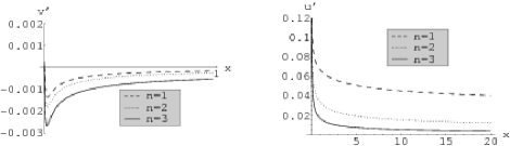
Figure 4.1: The solutions $v^{\prime}(x),u^{\prime}(x)$ for different $n$.

Notice that here we present the solutions for dotted values $v^{\prime}(=\tilde{v})$ and $u^{\prime}(=\tilde{u})$. The local DOS is shown schematically in Figs. 4.2, 4.3 for different $n$. The Fig. 4.3 describes also the dependence of the local DOS on a position of the maximum value of integrand in (4.9)(which actually characterizes the numerically calculated localization point of an electron).

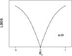
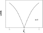
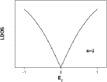
Figure 4.2: Schematic densities of states near the Fermi energy in the case of sphere.

Here and below $\delta=0.1$. Notice that in fact the choice of the value of $\delta$ does not influence the characteristic behavior of LDOS. As is seen, the DOS has a cusp which drops to zero at the Fermi energy. The case $n=3$ becomes distinguished. Let us emphasize once more that in the fullerene molecule there are twelve $60^{\circ}$ disclinations, so that the case $n=1$ is actually realized.

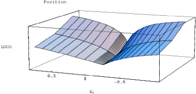
Figure 4.3: 3d schematic plotting of the DOS near the Fermi energy for $n=0,1,2$ (going from the front side to the back side).

Chapter 5 Spheroidal geometry approach to fullerenes

Geometry, topological defects and the peculiarity of graphene lattice have a pronounced effect on the electronic structure of fullerene molecules. The most extensively studied $C_{60}$ molecule is an example of a spherical fullerene nicknamed a ”soccer ball” [40]. Moreover, the spherical fullerenes as $C_{60}$ are stable towards fragmentation than the other bigger fullerenes [41]. The family of icosahedral spherical fullerenes is described by the formula $20(n^{2}+nl+l^{2})$ with integer $n$ and $l$. Other fullerenes are either slightly (as $C_{70}$) or remarkably deformed and their general nickname is a ”rugby ball”. The electronic structure of $C_{70}$ cluster of $D_{5h}$ geometry has been studied in [42] by using the local-density approximation in the density-functional theory. It was clearly shown that the spheroidal geometry is of a decisive importance for observed peculiarities in electronic states of the $C_{70}$. What is important, the calculated energy levels were found to be in good agreement with photoemission experiments. Spheroidal fullerenes can be considered as a initially flat hexagonal network which has warped into closed monosurface by twelve disclinations. We are interested here in the slightly elliptically deformed big fullerenes like C₂₄₀ and C₅₄₀ molecules, see Figures 5.1, 5.2 [40].

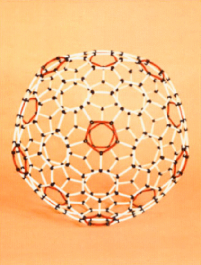
Figure 5.1: Picture of molecular model of giant spheroidal fullerene $C_{240}$.

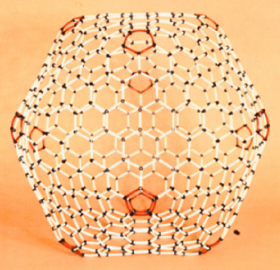
Figure 5.2: Picture of molecular model of giant spheroidal fullerene $C_{540}$.

It should be noted that the formulation of any continuum model begins from the description of a graphite sheet (graphene) (see, e.g., [10, 15, 11, 43, 12, 44]). The models which involve the influence of both geometry and topological defects on the electronic structure by boundary conditions were developed in Refs. [45, 46]. A different variant of the continuum model within the effective-mass description for fullerene near one pentagonal defect was suggested in previous section. There are attempts to describe electronic structure of the graphene compositions by the Dirac-Weyl equations on the curved surfaces where the structure of the graphite with pentagonal rings taken into account is imposed with the help of the so-called $K$ spin contribution [14, 47]. In the case of spherical geometry, this is realized by introducing an effective field due to magnetic monopole placed at the center of a sphere [14]. In this section we use a similar approach. The difference is that we consider also the elastic contribution. Indeed, pentagonal rings being the disclination defects are the sources of additional strains in the hexagonal lattice. Moreover, the disclinations are topological defects and the elastic flow due to a disclination is determined by the topological Frank index. For this reason, this contribution exists even within the so-called ”inextensional” limit which is rather commonly used in description of graphene compositions (see, e.g., [48]).

Recently, in the framework of a continuum approach the exact analytical solution for the low energy electronic states in icosahedral spherical fullerenes has been found [49]. The case of elliptically deformed fullerenes was studied in [50] where some numerical results were presented. In this section, we suggest a similar to [49] model with the Dirac monopole instead of ’t Hooft-Polyakov monopole for describing elastic fields. We consider a slightly elliptically deformed sphere with the eccentricity of the spheroid $e\ll 1$. In this case, by analogy with [51] we use the spherical representation for the eigenstates, with the slight asphericity considered as a perturbation. This allows us to find explicitly the low-lying electronic spectrum for spheroidal fullerenes.

The problem of Zeeman splitting and Landau quantization of electrons on a sphere was studied in Ref. [52]. To this end, the Schrödinger equation for a free electron on the surface of a sphere in a uniform magnetic field was formulated and solved.Our studies also cover slightly elliptically deformed fullerenes influent by the weak uniform external magnetic field pointed in the different directions.

5.1 The model

Let us start with introducing spheroidal coordinates and writing down the Dirac operator for free massless fermions on the Riemannian spheroid $S^{2}$. The Euler’s theorem for graphene requires the presence of twelve pentagons to get the closed molecule. In a spirit of a continuum description we will extend the Dirac operator by introducing the Dirac monopole field with charge G inside the spheroid to simulate the elastic vortices due to twelve pentagonal defects. The $K$ spin flux which describes the exchange of two different Dirac spinors in the presence of a conical singularity will also be included in a form of t’Hooft-Polyakov monopole with charge g.

The Dirac equation on a surface $\Sigma$ in the presence of the abelian magnetic monopole field $W_{\mu}$ and the external magnetic field $A_{\mu}$ is written as [14, 47, 49]

$$i\gamma^{\alpha}e_{\alpha}^{\ \mu}[\nabla_{\mu}-iW_{\mu}-ia_{\mu}-iA_{\mu}]\psi=E\psi.$$ (5.1)

We impose the $K$ spin flux by the gauge field. In Cartesian coordinates

$$a_{x}=\frac{2gyz}{r(r^{2}-z^{2})}\tau_{2},\ a_{y}=\frac{-2gxz}{r(r^{2}-z^{2})}\tau_{2},\ a_{z}=0.$$ (5.2)

Disclination field we choose in the form

$$W_{x}=\frac{-Gy}{r(r+z)},\ W_{y}=\frac{Gx}{r(r+z)},\ W_{z}=0,$$ (5.3)

in the region $R_{N}$ (northern hemisphere) and

$$W_{x}=\frac{Gy}{r(r-z)},\ W_{y}=\frac{-Gx}{r(r-z)},\ W_{z}=0,$$ (5.4)

in the region $R_{S}$ (southern hemisphere). Here $r=\sqrt{x^{2}+y^{2}+z^{2}}$.

5.2 Electronic states near the Fermi energy in weak magnetic field pointed in the z direction

Firstly we will study the structure of electron levels near the Fermi energy influent by the weak magnetic field pointed in the $z$ direction (see Fig. 5.3) so that $\vec{A}=B\left(y,-x,0\right)/2$.

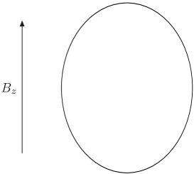
Figure 5.3: The schematic picture of the spheroidal fullerene in a weak uniform magnetic field pointed in the z direction.

The elliptically deformed sphere or a spheroid

$$\frac{x^{2}}{a^{2}}+\frac{y^{2}}{a^{2}}+\frac{z^{2}}{c^{2}}=1,$$ (5.5)

may be parameterized by two spherical angles $q^{1}=\phi$, $q^{2}=\theta$ that are related to the Cartesian coordinates $x$, $y$, $z$ as follows

$$x=a~{}\sin\theta\cos\phi;\quad y=a~{}\sin\theta\sin\phi;\quad z=c~{}\cos\theta.$$ (5.6)

The nonzero components of the metric tensor for spheroid are

$$g_{\phi\phi}=a^{2}\sin^{2}\theta;\quad g_{\theta\theta}=a^{2}\cos^{2}\theta+c^{2}\sin^{2}\theta,\quad$$ (5.7)

where $a,c\geq 0,~{}0\leq\theta\leq\pi,~{}0\leq\phi<2\pi$. Accordingly, orthonormal frame on spheroid is

$$e{{}_{1}}=\frac{1}{a~{}\sin\theta}~{}\partial_{\phi};\quad e{{}_{2}}=\frac{1}{\sqrt{a^{2}\cos^{2}\theta+c^{2}\sin^{2}\theta}}~{}\partial_{\theta}~{},$$ (5.8)

and dual frame reads

$$e{{}^{1}}=a~{}\sin\theta~{}d\phi;\quad e{{}^{2}}=\sqrt{a^{2}\cos^{2}\theta+c^{2}\sin^{2}\theta}~{}d{\theta}~{}.$$ (5.9)

A general representation for zweibeins is found to be

$$e{{}^{1}}_{\phi}=a~{}\sin\theta;\ e^{1}_{\ \theta}=0;\ e^{2}_{\ \phi}=0;\ e{{}^{2}}_{\theta}=\sqrt{a^{2}\cos^{2}\theta+c^{2}\sin^{2}\theta}~{}.$$ (5.10)

Notice that $e^{\mu}_{\ \alpha}$ is the inverse of $e^{\alpha}_{\ \mu}$. The Riemannian connection with respect to the orthonormal frame is written as [35, 53]

$$de^{1}=-\omega^{1}_{\ 2}\wedge e^{2}=\frac{a\cos\theta}{\sqrt{a^{2}\cos^{2}\theta+c^{2}\sin^{2}\theta}}\ d\phi\wedge e^{2},$$ (5.11)

$$de^{2}=-\omega^{2}_{\ 1}\wedge e^{1}=0.$$ (5.12)

Here $\wedge$ denotes the exterior product and $d$ is the exterior derivative. From Eqs. 5.11 and  5.12 we get the Riemannian connection in the form

$$\omega{{}_{\phi 2}^{1}}=-\omega{{}_{\phi 1}^{2}}=\frac{a\cos\theta}{\sqrt{a^{2}\cos^{2}\theta+c^{2}\sin^{2}\theta}}\ ;\quad\omega{{}_{\theta 2}^{1}}=\omega{{}_{\theta 1}^{2}}=0.$$ (5.13)

We assume that the eccentricity of the spheroid $e=\sqrt{|1-(c/a)^{2}|}$ is small enough. In this case, one can write down $c=a+\delta a$ where $\delta$ ($\mid\delta\mid\ll 1$) is a small dimensionless parameter characterizing the spheroidal deformation from the sphere. So, we can follow the perturbation scheme using $\delta$ as the perturbation parameter. Within the framework of the perturbation scheme the spin connection coefficients are written as

$$\omega{{}_{\phi 2}^{1}}=-\omega{{}_{\phi 1}^{2}}\approx\cos\theta(1-\delta\sin^{2}\theta),$$ (5.14)

where the terms to first order in $\delta$ are taken into account. The inclusion of the K-spin connection can be performed by considering two Dirac spinors as the two components of an $SU(2)$ color doublet $\psi=(\psi_{\uparrow}\psi_{\downarrow})^{T}$ (see Ref. [14] for details). In this case, the interaction with the color magnetic fields in a form of nonabelian magnetic flux (’t Hooft’-Polyakov monopole) is responsible for the exchange of the two Dirac spinors which in turn corresponds to the interchange of Fermi points. As was shown in Ref. [16], the Dirac equation for $\psi$ can be reduced to two decoupled equations for $\psi_{\uparrow}$ and $\psi_{\downarrow}$, which include an Abelian monopole of opposite charge, $g=\pm 3/2$.

The elastic flow through a surface due to a disclination has a vortex-like structure [13] and can be described by Abelian gauge field $W_{\mu}$. Similarly to Ref. [14], we replace the fields of twelve disclinations by the effective field of the magnetic monopole of charge $G$ located at the center of the spheroid. The circulation of this field is determined by the Frank index, which is the topological characteristic of a disclination. Trying to avoid an extension of the group we will consider the case of the Dirac monopole. The another possibility is to introduce the non-Abelian ’t Hooft-Polyakov monopole (see Ref. [49]). As is known, the vector potential $W_{\mu}$ around the Dirac monopole have singularities. To escape introducing singularities in the coordinate system let us divide the spheroid (similarly as it was done for the sphere in [54]) into two regions, $R_{N}$ and $R_{S}$, and define a vector potential $W_{\mu}^{N}$ in $R_{N}$ and a vector potential $W_{\mu}^{S}$ in $R_{S}$. Notice that below $W_{\mu}$ includes both gauge fields $W_{\mu}$ and $a_{\mu}$ defined in Eq. 5.1.

One has

$$R_{N}:\ \ 0\leq\theta<\frac{\pi}{2}+\Delta;\ 0\leq\phi<2\pi,$$

$$R_{S}:\ \ \frac{\pi}{2}-\Delta<\theta\leq\pi;\ 0\leq\phi<2\pi,$$

$$R_{NS}:\ \ \frac{\pi}{2}-\Delta<\theta<\frac{\pi}{2}+\Delta;\ 0\leq\phi<2\pi,\ (overlap)$$ (5.15)

where $\Delta$ is chosen from the interval $0<\Delta\leq\pi/2$. In spheroidal coordinates (5.7) the only nonzero components of $W_{\mu}$ are found to be

$$W^{N}_{\phi}\approx g\cos\theta(1+\delta\sin^{2}\theta)+G(1-\cos\theta)-\delta G\sin^{2}\theta\cos\theta,$$ (5.16)

$$W^{S}_{\phi}\approx g\cos\theta(1+\delta\sin^{2}\theta)-G(1+\cos\theta)-\delta G\sin^{2}\theta\cos\theta,$$ (5.17)

where the terms of an order of $\delta^{2}$ and higher are dropped. In the overlapping region the potentials $W_{\phi}^{N}$ and $W_{\phi}^{S}$ are connected by the gauge transformation

$$W_{\phi}^{N}=W_{\phi}^{S}+iS_{NS}\ \partial_{\phi}S^{-1}_{NS},$$ (5.18)

where

$$S_{NS}=e^{2iG\phi}$$

is the phase factor. The wavefunctions in the overlap $R_{NS}$ are connected by

$$\psi_{N}=S_{NS}\psi_{S},$$ (5.19)

where $\psi_{N}$ and $\psi_{S}$ are the spinors in $R_{N}$ and $R_{S}$, respectively. Since $S_{NS}$ must be single-valued [55], $2G$ takes integer values. Notice that the total flux due to Dirac monopole in Egs. 5.16 and  5.17 is equal to $4\pi G$. What is important, there is no contribution from the terms with $\delta$. In our case, the total flux describes a sum of elastic fluxes due to twelve disclinations, so that the total flux (the modulus of the total Frank vector) is equal to $12\times\pi/3=4\pi$. Therefore, one obtains $G=1$.

Let us consider the region $R_{N}$. In spheroidal coordinates, the only nonzero component of $W_{\mu}$ in region $R_{N}$ is found to be

$$W_{\phi}\approx g\cos\theta(1+\delta\sin^{2}\theta)+G(1-\cos\theta)-\delta G\sin^{2}\theta\cos\theta,$$ (5.20)

and the external magnetic field pointed in the z-direction reads

$$A_{\phi}=-\frac{1}{2}Ba^{2}\sin^{2}\theta.$$ (5.21)

By using the substitution (5.72) we obtain the Dirac equation for functions $u_{j}$ and $v_{j}$ in the form

$$\left(-i\sigma_{1}\frac{1}{a}(\partial_{\theta}+\frac{\cot\theta}{2})+\frac{\sigma_{2}}{a\sin\theta}\left(j-m\cos\theta+\frac{1}{2}Ba^{2}\sin^{2}\theta\right)+\delta\hat{\cal{D}}_{1}\right)\left(\begin{array}[]{c}u_{j}(\theta)\\ v_{j}(\theta)\\ \end{array}\right)$$

$$=E\left(\begin{array}[]{c}u_{j}(\theta)\\ v_{j}(\theta)\\ \end{array}\right),$$ (5.22)

where

$$\hat{\cal{D}}_{1}=-\frac{\gamma_{1}}{a}\sin\theta\left(j-2m\cos\theta\right)-\gamma_{1}\frac{Ba}{2}\sin^{3}\theta.$$ (5.23)

A convenient way to study the eigenvalue problem is to square Eq. (5.22). For this purpose, let us write the Dirac operator in Eq. (5.22) as $\hat{\cal{D}}=\hat{\cal{D}}_{0}+\delta\hat{\cal{D}}_{1}$. One can easily obtain that

$$\hat{\cal{D}}_{0}^{2} = -\frac{1}{a^{2}}\left(\partial^{2}_{\theta}+\frac{\cos\theta}{\sin\theta}\partial_{\theta}-\frac{1}{4}-\frac{1}{4\sin^{2}\theta}\right)+\frac{\left(j-m\cos\theta\right)^{2}}{a^{2}\sin^{2}\theta}+Bj+\frac{B}{2}\left(\sigma_{3}-2m\right)\cos\theta$$ (5.24)

$$+\sigma_{3}\frac{m-j\cos\theta}{a^{2}\sin^{2}\theta}+\frac{B^{2}a^{2}\sin^{2}\theta}{4}.$$

Notice that to first order in $\delta$ the square of the Dirac operator is written as $\hat{\cal{D}}^{2}=(\hat{\cal{D}}^{2}_{0}+\delta\hat{\Gamma}),$ where $\hat{\Gamma}=(\hat{\cal{D}}_{0}\hat{\cal{D}}_{1}+\hat{\cal{D}}_{1}\hat{\cal{D}}_{0}).$ In an explicit form

$$a^{2}\hat{\Gamma}=2j^{2}+jx\left(\sigma_{3}-6m\right)+4m(m-\sigma_{3})x^{2}+2m\sigma_{3}+3Ba^{2}(1-x^{2})x(\sigma_{3}/2-m)$$

$$+2Bja^{2}(1-x^{2})+B^{2}a^{4}(1-x^{2})^{2}/2,$$ (5.25)

where the appropriate substitution $x=\cos\theta$ is used. The equation $\hat{\cal{D}}^{2}\psi=E^{2}\psi$ takes the form

$$[\partial_{x}(1-x^{2})\partial_{x}-\frac{(j-mx)^{2}-j\sigma_{3}x+\frac{1}{4}+\sigma_{3}m}{1-x^{2}}-a^{2}BV(x)-\delta a^{2}\hat{\Gamma}]\left(\begin{array}[]{c}u_{j}(x)\\ v_{j}(x)\\ \end{array}\right)$$

$$=-(\lambda^{2}-\frac{1}{4})\left(\begin{array}[]{c}u_{j}(x)\\ v_{j}(x)\\ \end{array}\right),$$ (5.26)

where $\lambda=aE,V(x)=j+(\sigma_{3}-2m)x/2$. Since we consider the case of a weak magnetic field the terms with $B^{2}$ and $\delta B$ in Eq. (5.26) can be neglected. As a result, the energy spectrum for spheroidal fullerenes is found to be

$$(\lambda_{jn}^{\delta})^{2}=(n+|j|+1/2)^{2}-m^{2}+Ba^{2}\left(j+A_{jn}\right)+\delta\big{(}2j^{2}+A^{1}+A^{2}\big{)}$$ (5.27)

where

$$A_{jn}=-\frac{j(m^{2}-1/4)}{p(p+1)},$$

and

$$A^{1}=-\frac{j^{2}(6m^{2}-1/2)}{p(p+1)}+\frac{j^{2}m^{2}(4m^{2}-3)}{p^{2}(p+1)^{2}},$$ (5.28)

$$A^{2}=\frac{\left(4m(m-1)F_{n}(2\alpha,2\beta)-X\right)T\ J_{n}(2\alpha,2\beta)+\left(4m(m+1)F_{n}(2\mu,2\nu)+X\right)J_{n}(2\mu,2\nu)}{T\ J_{n}(2\alpha,2\beta)+J_{n}(2\mu,2\nu)}$$ (5.29)

$$X=\frac{2j^{2}m}{p(p+1)}+\frac{j^{2}m}{p^{2}(p+1)^{2}}-2m$$ (5.30)

$$F_{n}(2\alpha,2\beta)=\frac{(n+1)(n+2\alpha+1)(n+2\beta+1)(n+2\alpha+2\beta+1)}{(2p+1)(p+1)^{2}(2p+3)}$$ (5.31)

$$+\frac{n(n+2\alpha)(n+2\beta)(n+2\alpha+2\beta)}{(2p-1)p^{2}(2p+1)}$$

$$J_{n}(2\alpha,2\beta)=\Gamma(n+2\alpha+1)\Gamma(n+2\beta+1),$$

Here $p=n+\beta+\alpha$ and

$$T=\frac{n+\mid j\mid-m+1/2}{n+\mid j\mid+m+1/2}$$ (5.32)

When $\delta=0,B=0$, one has the case of a sphere with magnetic monopole inside. In this case, the exact solution is known (see, e.g., [49])

$$\left[\partial_{x}(1-x^{2})\partial_{x}-\frac{(j-mx)^{2}-j\sigma_{3}x+\frac{1}{4}+\sigma_{3}m}{1-x^{2}}\right]\left(\begin{array}[]{c}u_{jn}^{0}(x)\\ v_{jn}^{0}(x)\\ \end{array}\right)=-(\lambda^{2}_{0n}-\frac{1}{4})\left(\begin{array}[]{c}u_{jn}^{0}(x)\\ v_{jn}^{0}(x)\\ \end{array}\right),$$ (5.37)

$$\left(\begin{array}[]{c}u_{jn}^{0}\\ v_{jn}^{0}\\ \end{array}\right)=\left(\begin{array}[]{c}C_{u}(1-x)^{\alpha}(1+x)^{\beta}P_{n}^{2\alpha,2\beta}(x)\\ C_{v}(1-x)^{\mu}(1+x)^{\nu}P_{n}^{2\mu,2\nu}(x)\\ \end{array}\right),$$ (5.42)

with the energy spectrum

$$(\lambda_{jn}^{0})^{2}=(n+|j|+1/2)^{2}-m^{2}.$$ (5.43)

Here

$$\alpha=\frac{1}{2}\left|j-m-\frac{1}{2}\right|,\beta=\frac{1}{2}\left|j+m+\frac{1}{2}\right|,$$

$$\mu=\frac{1}{2}\left|j-m+\frac{1}{2}\right|,\nu=\frac{1}{2}\left|j+m-\frac{1}{2}\right|,$$ (5.44)

$P_{n}^{2\alpha,2\beta}(x)$ and $P_{n}^{2\mu,2\nu}(x)$ are Jacobi polynomials of $n$-th order, and $C_{u}$ and $C_{v}$ are the normalization factors. These states are degenerate. For example, the degeneracy of the zero mode is equal to six. Therefore, we have to use the perturbation scheme for the degenerate energy levels [56].

Finally, in the linear in $\delta$ approximation, the low energy electronic spectrum of spheroidal fullerenes takes the form

$$E_{jn}=E^{0}_{jn}+E^{\delta B_{z}}_{jn}$$ (5.45)

with

$$E^{0}_{jn}=\pm\sqrt{(2\xi+n)(2\eta+n)},$$

$$E^{\delta B_{z}}_{jn}=\frac{Ba^{2}(j+A_{jn})+\delta(2j^{2}+A^{1}+A^{2})}{2E^{0}_{jn}},$$ (5.46)

where $\xi=\mu\ (\nu)$ and $\eta=\beta\ (\alpha)$ for $j>0\ (j<0)$, respectively. The parameters $\alpha$, $\beta$, $\mu$, $\nu$ are defined above.

Here we came back to the energy variable $E=\lambda/a$ (in units of $\hbar V_{F}/a$ where $V_{F}$ is the Fermi velocity). Notice that the non-diagonal matrix element of perturbation $\langle e^{j\phi}|\langle\psi_{jn}|\Gamma|\psi_{-jn}\rangle|e^{-j\phi}\rangle$ turns out to be zero. Therefore, the states with opposite $j$ do not mix and $j$ remains a good quantum number as would be expected. As is seen from Eq. (5.45), for $\delta=0$ both eigenstates and eingenvalues are the same as for a sphere (cf. Ref. [49]). At the same time, Eqs. (5.45) and (5.46) show that the spheroidal deformation gives rise to an appearance of fine structure in the energy spectrum. The difference in energy between sublevels is found to be linear in $\delta$ which resembles the Zeeman effect where the splitting energy is linear in magnetic field. In addition we found a further splitting of the states with opposite $j$.

$YO-C_{240}$	$j$	$E^{0}_{jn}(eV)$	$E^{\delta}_{jn}(meV)(B=0)$	$E^{\delta B_{z}}_{jn}(meV)(Ba^{2}=0.1)$
$n=0$, $m=1/2$	1	1.094	10.5	37.5
	-1	1.094	10.5	-16.5
$n=1$, $m=1/2$	1	1.89	8.8	24.8
	-1	1.89	8.8	-7.2
$n=0$, $m=1/2$	2	1.89	28.4	60.4
	-2	1.89	28.4	-3.6
$n=0$, $m=-5/2$	3	1.89	3	27
	-3	1.89	3	-21

Table 5.1: The structure of the first and higher energy levels for YO-C₂₄₀ fullerene in uniform magnetic field. The hopping integral and other parameters are taken to be $t=2.5\ eV$ and $V_{F}=3t\overline{b}/2\hbar$, $\overline{b}=1.45{\textmd{\AA}}$, $\overline{R}=7.03{\textmd{\AA}}$, $SD=0.17{\textmd{\AA}}$, $\delta=0.024$. $\overline{b}$ is average bond length, $\overline{R}\ (\overline{R}=a)$ is average radius, $SD$ is standard deviation from a perfect sphere (see Refs. [57, 58]), so that $\delta=SD/\overline{R}$.

As an example, Table 5.1 shows all contributions (in compliance with Eq. (5.45)) to the first and second energy levels for YO-C₂₄₀ (YO means a structure given in [57, 58]). Schematically, the structure of the first energy level is shown in Fig. 5.4. As is clearly seen, the first (double degenerate) level becomes shifted due to spheroidal deformation and splitted due to nontrivial topology. The uniform magnetic field provides the well-known Zeeman splitting. The difference between topological and Zeeman splitting is clearly seen. In the second case, the splitted levels are shifted in opposite directions while for topological splitting the shift is always positive. The more delicate is the structure of the second level which is schematically presented in Fig. 5.5. In this case, the initial (for $\delta=0$) degeneracy of $E^{0}_{jn}$ is equal to six. The spheroidal deformation provokes an appearance of three shifted double degenerate levels (fine structure) which, in turn, are splitted due to the presence of topological defects. The magnetic field is responsible to Zeeman splitting.

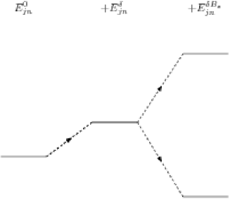
Figure 5.4: The schematic picture of the first positive electronic level $E_{jn}^{\delta}$ for spheroidal fullerenes in a weak uniform magnetic field pointed in the z direction.

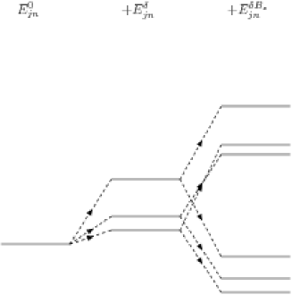
Figure 5.5: The schematic picture of the second positive electronic level $E_{jn}^{\delta}$ of the spheroidal fullerenes in a weak uniform magnetic field pointed in the z direction.

We admit that the obtained values of the splitting energies can deviate from the estimations within some more precise microscopic lattice models and density-functional methods (see, e.g.[59]). Therefore, we focused mostly on the very existence of physically interesting effects. For this reason, the values in both Table and the schematic pictures are presented with accuracy at about one percent of $E^{0}_{jn}$.

5.3 Electronic states near the Fermi energy in weak magnetic field pointed in the x direction

In the second case we introduce that the uniform external magnetic field $B$ is chosen to be pointed in the $x$ direction (see 5.6) so that $\vec{A}=B\left(0,-z,y\right)/2$.

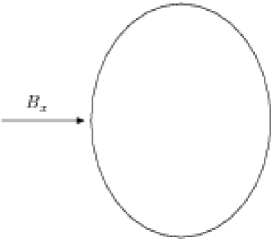
Figure 5.6: The schematic picture of the spheroidal fullerene in a weak uniform magnetic field pointed in the x direction.

The nonzero component of $W_{\mu}$ in region $R_{N}$ are the same as in previous case but the external magnetic field are changed

$$A_{\phi}=-\frac{1}{2}Bac\sin\theta\cos\theta\cos\phi,$$ (5.47)

$$A_{\theta}=-\frac{1}{2}Bac\sin\phi,$$ (5.48)

where $c=a+\delta a$ and only the terms to the first order in $\delta$ are taken into account. Following the calculations above with neglecting the terms $B^{2}$ and $\delta B$ we obtain the Dirac equation for functions $u_{j}$ and $v_{j}$ in the form

$$\left(-i\sigma_{1}\frac{1}{a}(\partial_{\theta}+\frac{\cot\theta}{2}+i\frac{1}{2}Ba^{2}\sin\phi)+\frac{\sigma_{2}}{a\sin\theta}\left(j-m\cos\theta+\frac{1}{2}Ba^{2}\sin\theta\cos\theta\cos\phi\right)+\delta\hat{\cal{D}}_{1}\right)\times$$

$$\times\left(\begin{array}[]{c}u_{j}(\theta)\\ v_{j}(\theta)\\ \end{array}\right)=E\left(\begin{array}[]{c}u_{j}(\theta)\\ v_{j}(\theta)\\ \end{array}\right),$$ (5.49)

where

$$\hat{\cal{D}}_{1}=-\frac{\gamma_{1}}{a}\sin\theta\left(j-2m\cos\theta\right)-\gamma_{1}\frac{Ba}{2}\sin^{2}\theta\cos\theta\cos\phi.$$ (5.50)

We find the square of nonperturbative part of Dirac operator above in the form

$$\hat{\cal{D}}_{0}^{2} = -\frac{1}{a^{2}}\left(\partial^{2}_{\theta}+\frac{\cos\theta}{\sin\theta}\partial_{\theta}-\frac{1}{4}-\frac{1}{4\sin^{2}\theta}\right)+\frac{\left(j-m\cos\theta\right)^{2}}{a^{2}\sin^{2}\theta}$$ (5.51)

$$+\sigma_{3}\frac{m-j\cos\theta}{a^{2}\sin^{2}\theta}+BV(\theta,\phi),$$

where the terms with $B^{2}$ and $\delta B$ was neglecting and

$$V(\theta,\phi) = -i(\cos\phi\partial_{\phi}-\frac{\sin\phi}{2})\cot\theta-\sigma_{3}\frac{\cos\phi(1+\sin^{2}\theta)}{2\sin\theta}-i(\partial_{\theta}+\frac{1}{2}\cot\theta)\sin\phi$$ (5.52)

$$-\frac{m\cos^{2}\theta\cos\phi}{\sin\theta}.$$

We denote $V_{j,j^{\prime}}^{m}=\langle\psi_{jn}^{m}|V(\theta,\phi)|\psi_{j^{\prime}n}^{m}\rangle$, where $\psi_{jn}^{m}$ are the eigenfunctions of $\hat{\cal{D}}_{0}$. In the case of first energy mode the terms $V_{-1,-1}^{1/2}$, $V_{1,1}^{1/2}$, $V_{1,-1}^{1/2}$, $V_{-1,1}^{1/2}$ are zero and therefore the weak magnetic field pointed in the x direction do not influent the first energy level. For the second energy mode only nondiagonal terms $V_{-1,-2}^{1/2}$, $V_{1,2}^{1/2}$ were find different from zero. The following numerical values of the nondiagonal terms $V_{j,j^{\prime}}^{m}$ was found: $V_{-1,-2}^{1/2}=-2.1$, $V_{1,2}^{1/2}=2.1$. We use the wave functions for calculations of nondiagonal terms in the case of second energy level in the form:

$$\psi_{0,2}^{1/2}(z,\phi)=\frac{e^{i2\phi}}{\sqrt{2\pi}}\sqrt{\frac{32}{15}}\left(\begin{array}[]{c}-i\sqrt{\frac{2}{3}}\sqrt{1-z^{2}}(1+z)\\ 1-z^{2}\\ \end{array}\right),$$ (5.55)

$$\psi_{0,-2}^{1/2}(z,\phi)=\frac{e^{-i2\phi}}{\sqrt{2\pi}}\sqrt{\frac{32}{15}}\left(\begin{array}[]{c}i\sqrt{\frac{2}{3}}\sqrt{1-z^{2}}(1-z)\\ 1-z^{2}\\ \end{array}\right),$$ (5.58)

$$\psi_{1,1}^{1/2}(z,\phi)=\frac{e^{i\phi}}{\sqrt{2\pi}}\sqrt{\frac{3}{5}}\left(\begin{array}[]{c}-i\sqrt{\frac{2}{3}}(2z^{2}+z-1)\\ \frac{3}{2}z\sqrt{1-z^{2}}\\ \end{array}\right),$$ (5.61)

$$\psi_{1,-1}^{1/2}(z,\phi)=\frac{e^{-i\phi}}{\sqrt{2\pi}}\sqrt{\frac{3}{5}}\left(\begin{array}[]{c}i\sqrt{\frac{2}{3}}(-2z^{2}+z+1)\\ \frac{3}{2}z\sqrt{1-z^{2}}\\ \end{array}\right).$$ (5.64)

The low energy electronic spectrum of spheroidal fullerenes in this case takes the form

$$E_{jn}=E^{0}_{jn}+E^{\delta B_{x}},$$ (5.65)

where

$$E^{\delta B_{x}}=\frac{\delta\left(\hat{\Gamma}_{22}+\hat{\Gamma}_{11}\right)\pm\sqrt{\delta^{2}\left(\hat{\Gamma}_{22}-\hat{\Gamma}_{11}\right)^{2}+4|Ba^{2}V_{1,2}|^{2}}}{4E^{0}_{jn}}.$$ (5.66)

We change $1,2$ to $-1,-2$ in the expression above to get the another energy levels in the degenerate energy state which is considered. Where the $\hat{\Gamma}_{ii}$ are the diagonal matrix element of perturbation of Eq. 5.25 with $B=0$. Table 5.2 shows all contributions to the first and second energy levels for YO-C₂₄₀ fullerenes influent by the horizontal weak external magnetic field. Figures 5.7, 5.8 present first and second positive energy levels of spheroidal fullerenes in weak magnetic field pointed in the x direction in comparison with Figures 5.4, 5.5. As is seen, there is a marked difference between the behavior of the first and second energy levels in magnetic field. Indeed, in both cases the energy levels become shifted due to spheroidal deformation. However, the uniform magnetic field does not influence the first energy level. The splitting takes place only for the second level. We can conclude that there is a possibility to change the structure of the electronic levels in spheroidal fullerenes by altering the direction of magnetic field. It would be interesting to test this prediction in experiment. The values in both Table and the schematic pictures are presented the same way as in the previous case with accuracy at about one percent of $E^{0}_{jn}$.

$YO-C_{240}$	$j$	$E^{0}_{jn}(eV)$	$E_{jn}^{\delta}(meV)(B=0)$	$E_{jn}^{\delta B_{x}}(meV)(Ba^{2}=0.1)$
$n=0$, $m=1/2$	1	1.094	10.5	10.5
	-1	1.094	10.5	10.5
$n=0$, $m=-5/2$	3	1.89	3	3
	-3	1.89	3	3
$n=0$, $m=1/2$	2	1.89	28.4
				53/-16/
$n=1$	1	1.89	8.8
$n=1$, $m=1/2$	-1	1.89	8.8
				53/-16/
$n=0$	-2	1.89	28.4

Table 5.2: The structure of the first and second energy levels for YO-C₂₄₀ fullerene in uniform magnetic field. The hopping integral and other parameters are taken to be $t=2.5\ eV$ and $V_{F}=3t\overline{b}/2\hbar$, $\overline{b}=1.45{\textmd{\AA}}$, $\overline{R}=7.03{\textmd{\AA}}$, $SD=0.17{\textmd{\AA}}$, $\delta=0.024$. $\overline{b}$ is average bond length, $\overline{R}\ (\overline{R}=a)$ is average radius, $SD$ is standard deviation from a perfect sphere (see Refs. [57, 58]), so that $\delta=SD/\overline{R}$.

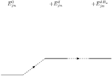
Figure 5.7: The schematic picture of the first positive electronic level $E_{jn}^{\delta}$ for spheroidal fullerenes in a weak uniform magnetic field pointed in the x direction.

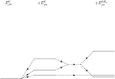
Figure 5.8: The schematic picture of the second positive electronic level $E_{jn}^{\delta}$ with a mixture of quantum numbers $j=1,2$ and $j=-1,-2$ for spheroidal fullerenes in a weak uniform magnetic field pointed in the x direction.

5.4 Zero-energy mode

Now we will analyze the special case of an electron state at the Fermi level (so-called zero-energy mode), in this case the right side of equation 5.1 is equal to zero. We will use the projection coordinates in the form

$$x=\frac{2R^{2}r}{R^{2}+r^{2}}\cos\phi;\quad y=\frac{2R^{2}r}{R^{2}+r^{2}}\sin\phi;\quad z=-c\frac{R^{2}-r^{2}}{R^{2}+r^{2}},$$ (5.67)

where $R$ and $c$ are the spheroidal axles. The Riemannian connection with respect to the orthonormal frame is written as [35, 53]

$$-\omega{{}_{\phi 2}^{1}}=\omega{{}_{\phi 1}^{2}}=\frac{R^{2}-r^{2}}{\sqrt{(R^{2}-r^{2})^{2}+4c^{2}r^{2}}}\ ;\quad\omega{{}_{r2}^{1}}=\omega{{}_{r1}^{2}}=0.$$ (5.68)

The only nonzero component of the gauge field $W_{\mu}$ in region $R_{N}$ for spheroidal fullerenes reads

$$W_{\phi}=G+m\frac{z}{X},$$ (5.69)

where

$$X=\frac{\sqrt{c^{2}(r^{2}-R^{2})^{2}+4R^{4}r^{2}}}{r^{2}+R^{2}}.$$ (5.70)

Notice that the monopole field $W_{\mu}$ in Eq. (5.69) consists of two parts. The first one comes from the $K$-spin connection term and implies the charge $g=\pm 3/2$ while the second one is due to elastic flow through a surface. This contribution is topological in its origin and characterized by charge $G$. For total elastic flux from twelve pentagonal defects one has $G=1$. The parameter $m=g-G$ is introduced in Eq.(5.69). The uniform external magnetic field $B$ for simplicity is chosen to be pointed in the $z$ direction. In projection coordinates the only nonzero component of $A_{\mu}$ is written as

$$A_{\phi}=-\frac{2BR^{4}r^{2}}{(R^{2}+r^{2})^{2}}.$$ (5.71)

Let us study Eq.(5.1) for the electronic states at the Fermi energy ($E=0$). The Dirac matrices can be chosen to be the Pauli matrices, $\gamma_{1}=-\sigma_{2},\gamma_{2}=-\sigma_{1}$. By using the substitution

$$\left(\begin{array}[]{c}\psi_{A}\\ \psi_{B}\\ \end{array}\right)=\sum_{j}\frac{e^{i(j+G)\phi}}{\sqrt{2\pi}}\left(\begin{array}[]{c}u_{j}(r)\\ v_{j}(r)\\ \end{array}\right),j=0,\pm 1,\pm 2,\ldots$$ (5.72)

we obtain

$$\left(\frac{1}{r}(j-m\frac{z}{X}-A_{\phi})+\frac{R^{2}+r^{2}}{K}(\partial_{r}-\frac{r^{2}-R^{2}}{2r(r^{2}+R^{2})})\right)v(r)=0,$$ (5.73)

$$\left(\frac{1}{r}(j-m\frac{z}{X}-A_{\phi})-\frac{R^{2}+r^{2}}{K}(\partial_{r}-\frac{r^{2}-R^{2}}{2r(r^{2}+R^{2})})\right)u(r)=0,$$ (5.74)

where $K=\sqrt{(R^{2}-r^{2})^{2}+4c^{2}r^{2}}$. We assume that the eccentricity of the spheroid is small enough. In this case, one can write down $c=R+\delta R$ and $\delta$ ($\mid\delta\mid\ll 1$) is a small dimensionless parameter characterizing the spheroidal deformation. Therefore, one can follow the perturbation scheme using $\delta$ as the perturbation parameter. To the leading in $\delta$ approximation Eqs. (5.73) and (5.74) are written as

$$\partial_{r}v_{j}(r)=(-\frac{(R^{2}+r^{2})^{2}}{r[(R^{2}+r^{2})^{2}-4R^{2}r^{2}\delta]}[j-m(1+\delta)\frac{r^{2}-R^{2}}{r^{2}+R^{2}}+m\delta\frac{(r^{2}-R^{2})^{3}}{(r^{2}+R^{2})^{3}}]$$

$$-\frac{2BR^{4}r}{[(R^{2}+r^{2})^{2}-4R^{2}r^{2}\delta]}+\frac{r^{2}-R^{2}}{2r(R^{2}+r^{2})})v_{j}(r),$$ (5.75)

$$\partial_{r}u_{j}(r)=(\frac{(R^{2}+r^{2})^{2}}{r[(R^{2}+r^{2})^{2}-4R^{2}r^{2}\delta]}[j-m(1+\delta)\frac{r^{2}-R^{2}}{r^{2}+R^{2}}+m\delta\frac{(r^{2}-R^{2})^{3}}{(r^{2}+R^{2})^{3}}]$$

$$+\frac{2BR^{4}r}{[(R^{2}+r^{2})^{2}-4R^{2}r^{2}\delta]}+\frac{r^{2}-R^{2}}{2r(R^{2}+r^{2})})u_{j}(r).$$ (5.76)

The exact solution to Eqs. (5.75) and (5.76) is found to be

$$v_{j}(x)=\frac{(x+1)^{(1/2-m)}}{x^{\frac{1}{2}(j+m+1/2)}}\left(\frac{x+1-2\delta-2\sqrt{\delta(\delta-1)}}{x+1-2\delta+2\sqrt{\delta(\delta-1)}}\right)^{-\alpha}\left((x+1)^{2}-4\delta x\right)^{m},$$ (5.77)

$$u_{j}(x)=(x+1)^{(m+1/2)}x^{\frac{1}{2}(j+m-1/2)}\left(\frac{x+1-2\delta-2\sqrt{\delta(\delta-1)}}{x+1-2\delta+2\sqrt{\delta(\delta-1)}}\right)^{\alpha}\left((x+1)^{2}-4\delta x\right)^{-m},$$ (5.78)

where $x=r^{2}/R^{2}$, $\alpha=(j/2)\sqrt{\delta/(\delta-1)}+BR^{2}/4\sqrt{\delta(\delta-1)}$. The function $u_{j}$ can be normalized if the condition $m-1/2<j<1/2-m$ is fulfilled. In turn, the normalization condition for $v_{j}$ has the form $-1/2-m<j<m+1/2$. Finally, there are five normalized solutions for $u_{j}$ with $j=0,\pm 1,\pm 2$ when $m=-5/2$, and one solution for $v_{j}$ with $j=0$ when $m=1/2$. In the limit $\delta\rightarrow 0$ we arrive at the solution for spherical fullerenes

$$v_{j}(r)=r^{(-1/2-j-m)}(R^{2}+r^{2})^{(1/2+m)}e^{\frac{BR^{4}}{R^{2}+r^{2}}},$$

$$u_{j}(r)=r^{(-1/2+j+m)}(R^{2}+r^{2})^{(1/2-m)}e^{-\frac{BR^{4}}{R^{2}+r^{2}}}.$$ (5.79)

Since normalization conditions do not depend on the parameter $\delta$ they are the same as for spherical case. Thus the perturbation does not change the number of zero modes. Notice that Eq. (5.79) can be obtained from Eqs. (5.77) and (5.78) by using $\lim\left[1+(x/a)\right]^{a}=e^{x},a\rightarrow\infty$. Because of the different behaviour of the zero-energy modes there is also possibility to recognize the zero-eigenvalue states in experiment.

5.5 The $SU(2)$ algebra

The angular-momentum operators for Dirac operator on the sphere $S^{2}$ with charge $G$ and total magnetic monopole $m$ looks as follows

$$\hat{L}_{z}=-i(\partial_{\phi}\mp iG),$$ (5.80)

$$\hat{L}_{x}=i\sin\phi\partial_{\theta}+i\cos\phi\frac{\cos\theta}{\sin\theta}\left(\partial_{\phi}\mp iG-i\frac{m}{\cos\theta}\right)+\sigma_{z}\frac{\cos\phi}{2\sin\theta},$$ (5.81)

$$\hat{L}_{y}=-i\cos\phi\partial_{\theta}+i\sin\phi\frac{\cos\theta}{\sin\theta}\left(\partial_{\phi}\mp iG-i\frac{m}{\cos\theta}\right)+\sigma_{z}\frac{\sin\phi}{2\sin\theta},$$ (5.82)

where $-(+)$ sign correspond to north (south) hemisphere. These operators satisfy the standard commutations relations of the $SU(2)$ algebra:

$$\varepsilon_{ijk}\hat{L}_{j}\hat{L}_{k}=i\hat{L}_{i}.$$ (5.83)

The square of Dirac operator and $\hat{L}^{2}$ may be diagonalized simultaneously

$$\hat{\cal{D}}_{0}^{2}(B=0)=\hat{L}^{2}+\frac{1}{4}-m^{2}.$$ (5.84)

We can see that the operator $V(\theta,\phi)$ in the case when the magnetic field is pointed in the z direction can be expressed in the form

$$V(\theta,\phi)=\hat{L_{z}}+\left(\frac{\sigma_{3}}{2}-m\right)z.$$ (5.85)

In the case when the magnetic field is pointed in the x direction we have

$$V(\theta,\phi)=-\hat{L_{x}}-\left(\frac{\sigma_{3}}{2}-m\right)x,$$ (5.86)

where x,z are Cartesian coordinate

$$x=\sin\theta\cos\phi;\quad z=\cos\theta.$$ (5.87)

The square of Dirac operator and operator $\hat{L}^{2}$ may be diagonalized simultaneously and their eigenvalues are interrelated

$$\langle E,n|\hat{L}^{2}|E,n\rangle=l(l+1)=E^{2}-\frac{1}{4}=(n+|j|)(n+|j|+1),$$ (5.88)

where

$$l=n+|j|.$$ (5.89)

We can use instead of $n$ the angular momentum $l=n+|j|$. We can introduce the eigensteite of $\hat{\cal{D}}_{0}(B=0)$ in the form

$$\Psi_{l,j}(x,\phi)=\frac{e^{i(j\pm G)\phi}}{\sqrt{2\pi}\Omega}\sqrt{\frac{(l+j)!}{(l-j)!}}$$

$$\times\left(\begin{array}[]{c}(1-x)^{-\frac{1}{2}(j-m-1/2)}(1+x)^{-\frac{1}{2}(j+m+1/2)}\frac{d^{l-j}}{dx^{l-j}}(1-x)^{(l-m-1/2)}(1+x)^{(l+m+1/2)}\\ isgn(E)(1-x)^{-\frac{1}{2}(j-m+1/2)}(1+x)^{-\frac{1}{2}(j+m-1/2)}\frac{d^{l-j}}{dx^{l-j}}(1-x)^{(l-m+1/2)}(1+x)^{(l+m-1/2)}\end{array}\right)$$ (5.90)

where

$$\Omega=2^{l}\sqrt{\Gamma(l-m+1/2)^{2}+\Gamma(l+m+1/2)^{2}},$$ (5.91)

and $\Gamma$ are the Gamma functions (see Ref. [60]). When we act by $L_{-}$ and $L_{+}$ on $\Psi$ we find that

$$\hat{L}_{-}\Psi_{l,j}=\sqrt{(l+j)(l-j+1)}\Psi_{l,j-1},$$ (5.92)

$$\hat{L}_{+}\Psi_{l,j}=\sqrt{(l+j+1)(l-j)}\Psi_{l,j+1},$$ (5.93)

where

$$\hat{L}_{-}=-e^{-i\phi}\left(\partial_{\theta}-i\frac{\cos\theta}{\sin\theta}\left(\partial_{\phi}\mp iG-i\frac{m}{\cos\theta}\right)-\frac{\sigma_{z}}{2\sin\theta}\right),$$ (5.94)

$$\hat{L}_{+}=e^{i\phi}\left(\partial_{\theta}+i\frac{\cos\theta}{\sin\theta}\left(\partial_{\phi}\mp iG-i\frac{m}{\cos\theta}\right)+\frac{\sigma_{z}}{2\sin\theta}\right).$$ (5.95)

Now we would like to transform our formulae to the cartesian coordinates. The corresponding transformation rules for spinors are [60]

$$(\Psi)_{C}=V^{{\dagger}}\Psi,$$ (5.96)

and cartesian realization of operator $\hat{L}$ is

$$\hat{L}_{C}=V^{{\dagger}}\hat{L}V,$$ (5.97)

with $V$-matrices given by

$$V=\exp\left(\frac{i\sigma_{y}}{2}\theta\right)\exp\left(\frac{i\sigma_{z}}{2}\phi\right).$$ (5.98)

For example we present the Cartesian realization of $\hat{L}_{x}$ operator

$$(\hat{L}_{x})_{C}=i\sin\phi\partial_{\theta}+i\cos\phi\frac{\cos\theta}{\sin\theta}\left(\partial_{\phi}\mp iG-i\frac{m}{\cos\theta}\right)+\frac{\sigma_{x}}{2},$$ (5.99)

that may be expressed in the form ($m=G=0$)

$$(\hat{L}_{x})_{C}=y\hat{p}_{z}-z\hat{p}_{y}+\frac{\sigma_{x}}{2}.$$ (5.100)

Chapter 6 Conclusion

Electronic properties of fullerenes molecules have been discussed from a theoretical point of view. The effective-mass approximation is particularly suitable for understanding global and essential features. In this scheme, the motion of electrons in fullerenes is described by Dirac-Weyl’s equation. The geometry and topology is found to influence the main physical characteristics of graphite nanoparticles, first of all, their electronic properties. The topological defects (disclinations) appear as generic defects in closed carbon structures.

We have considered the electronic states of spheroidal fullerenes provided the spheroidal deformation from the sphere is small enough. In this case, the spherical representation is used for describing the eigenstates of the Dirac equation, with the slight asphericity considered as a perturbation. The using of the perturbation scheme allows us to find the exact analytical solution of the problem. In particular, the energy spectrum of spheroidal fullerenes is found to possess the fine structure in comparison with the case of the spherical fullerenes. We have shown that this structure is weakly pronounced and entirely dictated by the topological defects, that is it has a topological origin. We found three twofold degenerate modes near the Fermi level with one of them being the true zero mode therefore our finding confirms the results of [42] that there can exist only up to twofold degenerate states in the $C_{70}$.

Notice that for spherical fullerenes ($\delta=0$) our results agree with those found in [49]. It is interesting that the predictions of the continuum model for spherical fullerenes are in qualitative agreement with tight-binding calculations [61, 62, 63, 64]. In particular, the energy gap between the highest-occupied and lowest-unoccupied energy levels becomes more narrow as the size of fullerenes becomes larger. It is important to keep in mind, however, that the continuum model itself is correct for the description of the low-lying electronic states. In addition, the validity of the effective field approximation for the description of big fullerenes is also not clear yet. Actually, this approximation allows us to take into account the isotropic part of long-range defect fields. For bigger fullerenes, one has to consider the anisotropic part of the long-range fields, the influence of the short-range fields due to single disclinations as well as the multiple-shell structure.

We have focused also on the structure of low energy electronic states of spheroidal fullerenes in the weak uniform magnetic field. For the states at the Fermi level, we found an exact solution for the wave functions. It is shown that the external magnetic field modifies the density of electronic states and does not change the number of zero modes. For non-zero energy modes, electronic states near the Fermi energy of spheroidal fullerene are found to be splitted in the presence of a weak uniform magnetic field. The case of the x-directed magnetic field was considered and compared with the case of the z-th direction. The z axis is defined as the rotational axis of the spheroid with maximal symmetry. The most important finding is that the splitting of the electronic levels depends on the direction of the magnetic field. Our consideration was based on the using of the eigenfunctions of the Dirac operator on the spheroid, which are also the eigenfunction of $\hat{L}_{z}$. Let us discuss this important point in more detail.

In the case of a sphere there is no preferable direction in the absence of the magnetic field. The magnetic field sets a vector, so that the z-axis can be oriented along the field. In this case, one has to use such eigenfunctions of the Dirac operator which are also the eigenfunctions of $\hat{L}_{z}$. For the x-directed magnetic field, the eigenfunction of both the Dirac operator and $\hat{L}_{x}$ must be used. Evidently, the same results will be obtained in both cases.

The situation differs markedly for a spheroid. The spheroidal symmetry itself assumes the preferential direction which can be chosen as the z-axis. In other words, the external magnetic field does not define the preferable orientation. The symmetry is already broken and, as a result, the case of the magnetic field pointed in the $x$ direction differs from the case of the $z$-directed field. For instance, there are no eigenfunctions which would be simultaneously the eigenfunctions of both the Dirac operator on the spheroid and $\hat{L}_{x}$. For this reason, the structure of the electronic levels is found to crucially depend on the direction of the external magnetic field (Figures 5.3-5.8).

It should be mentioned that the zero-energy states in our model corresponds to the HOMO (highest occupied molecular orbital) states in the calculations based on the local-density approximation in the density-functional theory (see, e.g. [42]). In particular, the HOMO-LUMO energy gap is found to be about $1.1$ eV for YO-C₂₄₀ fullerene within our model (here LUMO means the lowest unoccupied molecular orbital) [65, 66].

The very big fullerenes like C₉₆₀ and C₁₅₀₀ become more deformed, faceted and can no longer form a free-electron model like the electronic shell [67], which was the assumption for this model. For these structures the deviation from the sphericity is larger when the pentagon defects are localized at the opposite poles. In the case when the poles are far away from each other we obtain the structure of nanotubes, and for the exact description some new model related to that proposed here should be used. In our opinion, our predictions are quite general for the fullerene family and are of interest for experimental studies. Finally, we think that the spheroidal geometry approach especially our established generic models could also be related to other physical problems with slightly deformed spherical structures that are common in the nature e.g. in astrophysics for modeling pulsars or kvasars.

Acknowledgment

We would like to thank especially Prof. V. A. Osipov whose is also co-author our results presented in this review for usefully comments and advices during writing this chapter. The work was supported in part by VEGA grant 2/7056/27. of the Slovak Academy of Sciences, by the Science and Technology Assistance Agency under contract No. APVT-51-027904.

Bibliography

- [1] R. Rajaraman: Solitons and Instantons, (North-Holland, Amsterdam 1982)
- [2] V.A. Osipov: Phys. Lett. A 164 (1992) 327
- [3] H.W. Kroto, J.R. Heath, S.C. O’Brien et al.: Nature 318 (1985) 162
- [4] W. Kratschmer, L.D. Lamb, K. Fostiropoulos et al.: Nature 347 (1990) 354
- [5] S. Iijima: Nature 354 (1991) 56
- [6] T.W. Ebbesen: Physics Today, (June) (1996) 26
- [7] S. Iijima, T.Ichihashi, Y.Ando: Nature 356 (1992) 776
- [8] R.Saito, G.Dresselhaus, M.S.Dresselhaus: Phys. Rev. B 53 (1996) 2044
- [9] H. Terrones, M. Terrones: Carbon 36 (1998) 725
- [10] D.P. DiVincenzo, E.J. Mele: Phys. Rev. B 29 (1984) 1685
- [11] P.R. Wallace, Phys. Rev. 71 (1947) 622
- [12] J.C. Slonczewski and P.R. Weiss, Phys. Rev. 109 272 (1958) 272
- [13] V.A. Osipov, E.A. Kochetov: JETP Lett. 72 (2000) 199
- [14] J. González, F. Guinea, M.A.H. Vozmediano: Nucl.Phys. B 406 (1993) 771
- [15] C.L. Kane, E.J. Mele: Phys. Rev. Lett. 78 (1997) 1932
- [16] J. González, F. Guinea, M.A.H. Vozmediano: Phys. Rev. Lett. 69 (1992) 172
- [17] T.Ando: J.Phys.Soc. Jpn.74 (2005) 777
- [18] J.G. Hou, J. Yang, H. Wang et al.: Phys. Rev. Lett. 83 (1999) 3001
- [19] D.L. Carroll, P. Redlich, P.M. Ajayan et al.: Phys. Rev. Lett. 78 (1997) 2811
- [20] P. Kim, T.W. Odom, J.-L. Huang et al.: Phys. Rev. Lett. 82 (1999) 1225
- [21] B. An, S. Fukuyama, K. Yokogawa et al.: Appl. Phys. Lett. 78 (2001) 3696
- [22] S. Berber, Y.-K. Kwon, D. Tománek: Phys. Rev. B 62 (2000) R2291
- [23] V.A. Osipov, E.A. Kochetov, M. Pudlak: JETP 96 (2003) 140
- [24] K. Kobayashi: Phys. Rev. B 61 (2000) 8496
- [25] J.-C. Charlier, G.-M. Rignanese: Phys. Rev. Lett. 86 (2001) 5970
- [26] T. Yaguchi, T. Ando: J.Phys.Soc.Jpn. 71 (2002) 2224
- [27] R. Jackiw, C. Rebbi: Phys. Rev. D 16 (1977) 1052
- [28] R. Jackiw, J.R. Schrieffer: Nucl. Phys. B 190 (1981) 253
- [29] M.M. Salomaa, G.E. Volovik: Rev. Mod. Phys. 59 (1987) 533
- [30] R. Jackiw: Phys. Rev. D 29 (1984) 2375
- [31] G.E. Volovik: JETP Lett. 70 (1999) 792
- [32] J.M.Luttinger, Phys.Rev.84 (1951) 814
- [33] P.E. Lammert, V.H. Crespi: Phys. Rev. Lett. 85 (2000) 5190
- [34] V.A. Osipov, E.A. Kochetov: JETP Lett. 73 (2001) 631
- [35] M. Nakahara, Geometry, Topology and Physics, (Institute of Physics Publishing Bristol 1998)
- [36] N.D. Birrell and P.C.W. Davies, Quantum Fields in Curved Space, (Cambridge 1982)
- [37] E.A. Kochetov, V.A. Osipov: J.Phys. A: Math.Gen. 32 (1999) 1961
- [38] R. Pincak, V.A. Osipov: Phys. Lett. A 314 (2003) 315
- [39] B.A. Ovrut, S. Tomas: Phys.Rev. D 43 (1991) 1314
- [40] H. Kroto, Reviews of Modern Physics, 69 (1997) 703
- [41] R.T. Chancey et al., Phys. Rev. A 67 (2003) 043203
- [42] S. Saito and A. Oshiyama, Phys. Rev. B 44 (1991) 11532
- [43] W.H. Lomer, Proc. Roy. Soc. (London) A227 (1955) 330
- [44] J.M. Luttinger and Kohn, Phys. Rev. 97 (1955) 869
- [45] H. Matsumura and T. Ando, J. Phys. Soc. Jpn. 67 (1998) 3542
- [46] R. Saito, G. Dresselhaus and M.S. Dresselhaus, Physical Properties of Carbon Nanotubes (Imperial College Press, London, 2003)
- [47] P.E. Lammert and V.H. Crespi, Phys. Rev. B 69 (2004) 035406
- [48] J. Tersoff, Phys. Rev. B 46 (1992) 15546
- [49] D.V. Kolesnikov and V.A. Osipov, Eur.Phys.Journ. B 49 (2006) 465
- [50] R. Pincak, Phys. Lett. A 340 (2005) 267
- [51] K. Clemenger, Phys. Rev. B 32 (1985) 1359
- [52] H. Aoki and H. Suezawa, Phys. Rev. A 46 (1992) R1163
- [53] M.Göckeler and T.Schücker, Differential geometry, gauge theories, and gravity (Cambridge University Press 1989)
- [54] T.T.Wu and G.N.Yang, Nucl. Phys. B 107 (1976) 365
- [55] T.T.Wu and G.N.Yang, Phys. Rev. D 12 (1975) 3845
- [56] L.D. Landau and E.M. Lifshitz, Quantum Mechanics (Elsevier Science, Oxford, 2003)
- [57] M. Yoshida and E. Osawa, Fullerene Sci. Tech. 1 (1993) 55
- [58] J. P. Lu and W. Yang, Phys. Rev. B 49 (1994) 11421
- [59] R.A. Broglia, G. Colò, G. Onida, H.E. Roman, Solid State Physics of Finite Systems, (Springer 2004)
- [60] A.A. Abrikosov,jr., Int. Journ. of Mod. Phys. A 17 (2002) 885
- [61] A.Ch. Tang and F.Q. Huang, Phys. Rev. B 51 (1995) 13830
- [62] E. Manousakis, Phys. Rev. B 44 (1991) 10991
- [63] A. Perez-Garrido, F. Alhama and J.D. Catala, Chem. Phys. 278 (2002) 71
- [64] Y.L. Lin and F. Nori, Phys. Rev. B 49 (1994) 5200
- [65] M. Pudlak, R. Pincak and V.A. Osipov, Phys. Rev. B 74 (2006) 235435
- [66] M. Pudlak, R. Pincak and V.A. Osipov, Phys. Rev. A 75 (2007) 025201
- [67] N. Mizorogi et al., Chem. Phys. Lett. 378 (2003) 598