Heat Conduction Transport processes

Temperature dependence of thermal conductivity in 1D nonlinear lattices

Abstract

We examine the temperature dependence of thermal conductivity of one dimensional nonlinear (anharmonic) lattices with and without on-site potential. It is found from computer simulation that the heat conductivity depends on temperature via the strength of nonlinearity. Based on this correlation, we make a conjecture in the effective phonon theory that the mean-free-path of the effective phonon is inversely proportional to the strength of nonlinearity. We demonstrate analytically and numerically that the temperature behavior of the heat conductivity $\kappa\propto 1/T$ is not universal for 1D harmonic lattices with a small nonlinear perturbation. The computer simulations of temperature dependence of heat conductivity in general 1D nonlinear lattices are in good agreements with our theoretic predictions. Possible experimental test is discussed.

The role of nonlinearity in the dynamics of one dimensional (1D) nonlinear (anharmonic) lattices has attracted attention for many decades, for instance, the ergodicity problem in the Fermi-Pasta-Ulam (FPU) chains inducted by nonlinear interactions[1, 2], solitons in nonlinear partial differential equations[3] and discrete breathers in nonlinear lattices[4, 5], to name just a few. Recent years have witnessed increasing studies on the role of nonlinearity in heat conduction in low dimensional systems (See Ref.[6] and the references therein). The fundamental question is whether the non-integrability or chaos is an essential or a sufficient condition for the heat conduction to obey the Fourier law. From computer simulations, it is found that in some 1D nonlinear lattices such as the Frenkel-Kontorova (FK) model and the $\phi^{4}$ model, the heat conductivity is size independent[7, 8, 9]. Thus the heat conduction in these models obeys the Fourier’s law. This transport behavior is called normal heat conduction. Whereas in some other nonlinear lattices such as the FPU and alike models, the heat conduction exhibits anomalous behavior[10], namely the heat conductivity $\kappa$ diverges with the system size $N$ as $\kappa\sim N^{\delta}$. Studies in past years have focused on the physical origin and the value of the divergent exponent $\delta$[10, 11, 12, 13, 14]. It is found that the anomalous heat conduction is due to the anomalous diffusion and a quantitative connection between them has been established[15]. Most recently, a very general effective phonon theory has been proposed to describe the normal and anomalous heat conduction under the same framework[16].

As a by-product of the study of heat conduction in low dimensional systems, nonlinearity (anharmonicity) has been found very useful in controlling heat flow. Because of the nonlinearity, the lattice vibrational spectrum depends on temperature. This property has been used to design the thermal rectifiers/diodes[17, 18, 19, 20, 21, 22] and thermal transistors[23]. Inspired by the two segment theoretical models[18, 19], Chang et al [24] has built the first solid state thermal rectifier with a single walled carbon nanotube and boron nitride nanotube, which indicates the opening of a new research field - controlling heat flow at microscopic level by using nonlinearity.

However, in contrast to the size-dependence, the temperature dependence of heat conductivity and its relationship with the nonlinearity have not yet been studied systematically even though this problem is very fundamental and very important from the experimental point of view. In fact, for low dimensional nanoscale systems such as nanotube and nanowires etc, to measure the temperature dependence of thermal conductivity for a fixed length sample is much easier than that for the size dependence of thermal conductivity for a fixed temperature. The difficulty for measuring size-dependent thermal conductivities lies in the fabrication of low dimensional systems. One cannot guarantee that the systems (nanotube/nanowires) of different system sizes fabricated separately are identical. However, performing the experiments at different temperatures for a fixed length is feasible.

In this Letter, we study the temperature dependence of heat conductivity and its connection with nonlinearity in several representative 1D nonlinear lattices with and without on-site potential, namely, the FK model, the $\phi^{4}$ model, and the FPU models. We will show that the temperature dependence of heat conductivity cannot be understood by the phenomenological phonon collision theory[25] in harmonic lattice with a small nonlinear perturbation. We find via computer simulations that the heat conductivity is actually inversely proportional to the strength of nonlinearity. More interestingly, if we make a conjecture in the effective phonon theory that the mean-free-path of effective phonon is inversely proportional to the strength of nonlinearity, we can give a rather satisfactory explanation for the temperature dependence of heat conductivities at both weak and strong coupling regimes in 1D nonlinear lattices such as the FK and the FPU-$\beta$ models consistently. We argue that the results presented in the current paper can be tested by nano scale experiments.

Without loss of generality and simplicity, we consider a 1D nonlinear lattice whose Hamiltonian reads,

$$H=\sum^{N}_{i=1}\left[\frac{p^{2}_{i}}{2}+V(x_{i},x_{i+1})+U(x_{i})\right],$$ (1)

where $x_{i}$ is the displacement from the equilibrium position of the $i\it{th}$ particle. In the following study we consider both cases with on-site potential, such as the FK model and the $\phi^{4}$ model, and the cases without on-site potential such as the FPU-$\alpha$, the FPU-$\beta$ model and the FPU-$\alpha\beta$ model.

The Frenkel-Kontorova model In the FK model $V=\frac{1}{2}(x_{i}-x_{i+1})^{2}$, and $U=\frac{K}{(2\pi)^{2}}(1-\cos{2\pi x_{i}})$. In this Letter, we take parameter $K=2\pi$. The FK model is very special since it reduces to a harmonic lattice with a small nonlinear perturbation at both low and high temperature regimes. According to the phonon collision theory, the collision frequency of a given phonon should be proportional to the number of phonons with which it can collide. Since the phonon distribution function is proportional to $T$ in classical regime, the total number of excited phonons is proportional to $T$. Hence the mean-free-path of phonon $l\propto 1/T$. At this regime, the heat capacity and velocity of phonons are all constants. From the Debye formula, one gets the heat conductivity, $\kappa\propto l$. Therefore the heat conductivity, $\kappa\propto 1/T$ universally for the harmonic lattice with a small nonlinear perturbation.

We compute the heat conductivity of the FK model as a function of temperature with fixed boundary conditions and the Nose-Hoover heat baths. The results are shown in Fig.1 in double logarithmic scales. At the high temperature regime, the on-site potential is considered as a small perturbation, thus the FK model is suitable for the interpretation of phonon collision theory. However the heat conductivity in this regime is not inversely proportional to temperature $\kappa\propto 1/T$ as the phonon collision theory predicts, it increases almost linearly with the temperature $\kappa\propto T$! This striking contradictory suggests that the phonon collision theory may not be suitable to describe the classical heat transport.

To explain the temperature dependence of heat conductivity in 1D nonlinear lattices, we introduce a new quantity to describe the strength of nonlinearity. We define a dimensionless nonlinearity $\epsilon$ as a ratio between the average of nonlinear potential energy and the total potential energy which consists of linear and nonlinear potential energy:

$$\epsilon=\frac{\left|\langle E_{n}\rangle\right|}{\langle E_{l}+E_{n}\rangle},\,\,0\leq\epsilon\leq 1,$$ (2)

where $\langle\cdot\rangle$ is an ensemble average. For the harmonic lattice with a small nonlinear perturbation, the average of nonlinear potential energy $\langle E_{n}\rangle$ is negligible compared to the average of linear potential energy $\langle E_{l}\rangle$, thus the dimensionless nonlinearity can be approximated by $\epsilon\approx\frac{\left|\langle E_{n}\rangle\right|}{\langle E_{l}\rangle}$, where the average of the linear potential energy $\langle E_{l}\rangle=Nk_{B}T/2$ at the harmonic limit according to the theory of energy equipartition[26].

At the high temperature regime, the average of nonlinear on-site potential energy $\left<E_{n}\right>$ is negligible compared to the average of harmonic inter particle potential energy $\left<E_{l}\right>$. The dimensionless nonlinearity can be expressed as

$$\epsilon\approx\frac{\left<\sum_{i}\frac{1}{2\pi}\left(1-\cos{2\pi x_{i}}\right)\right>}{\left<\sum_{i}\frac{1}{2}\left(x_{i}-x_{i+1}\right)^{2}\right>}\propto\frac{N}{\left<\sum_{i}\frac{1}{2}\left(x_{i}-x_{i+1}\right)^{2}\right>},$$ (3)

where the average of the on-site potential energy of any particle, $\left<1-\cos{2\pi x_{i}}\right>$, has been assumed to be a constant in the interval $(0,2)$ at the high temperature regime. The average of inter particle potential energy $\left<\sum^{N}_{i=1}\frac{1}{2}\left(x_{i}-x_{i+1}\right)^{2}\right>=Nk_{B}T/2$. Therefore, the dimensionless nonlinearity at high temperature regime has the asymptotic behavior: $\epsilon\propto 1/T$. Compared with the computer simulation it is not difficult to find the correlation between the heat conductivity and the dimensionless nonlinearity at the high temperature regime for the FK model:

$$\kappa\propto\frac{1}{\epsilon}\propto T.$$ (4)

This correlation strongly suggests that the mean-free-path of phonons should be proportional to the inverse of the dimensionless nonlinearity, $l\propto 1/\epsilon$, rather than to the inverse of temperature, $l\propto 1/T$, as the phonon collision theory predicts.

As for the nonlinear lattice, the notion of phonon is not valid any more, one should invoke the effective phonon theory[16]. Recently, we find out that the normal and anomalous heat conduction can be treated with effective phonon theory[16]. For a general 1D nonlinear lattice with

$$V(x_{i},x_{i+1})=\sum^{\infty}_{s=2}g_{s}\frac{\left(x_{i}-x_{i+1}\right)^{s}}{s},U(x_{i})=\sum^{\infty}_{s=2}\sigma_{s}\frac{x^{s}_{i}}{s},$$ (5)

the spectrum of effective phonons is $\hat{\omega}^{2}_{k}=\alpha(\omega^{2}_{k}+\gamma)$, where $\omega=2\sqrt{g_{2}}\sin{k/2}$ is the phonon dispersion of harmonic lattice, and the temperature dependent coefficients $\alpha$ and $\gamma$ are defined as

$$\alpha=\frac{\sum_{s}g_{s}\langle\sum_{i}(x_{i}-x_{i+1})^{s}\rangle}{\langle\sum_{i}(x_{i}-x_{i+1})^{2}\rangle},\gamma=\frac{1}{\alpha}\frac{\sum_{s}\sigma_{s}\langle\sum_{i}x^{s}_{i}\rangle}{\langle\sum_{i}x^{2}_{i}\rangle}.$$ (6)

The heat conductivity can be expressed by the modified Debye formula:

$$\kappa=\frac{c}{2\pi}\int^{2\pi}_{0}P(k)v(k)l(k)dk,$$ (7)

where $c$ is the specific heat, $P(k)$ the normalized power spectrum of total heat flux, $v(k)=\partial{\hat{\omega}_{k}}/\partial{k}$ the velocity of the effective phonon, and $l(k)$ the mean-free-path of effective phonon. $l(k)=v(k)\tau(k)$, where $\tau(k)$ is the effective phonon relaxation time which is proportional to the quasi-period of effective phonons, $\tau(k)=\lambda 2\pi/\hat{\omega}_{k}$, and the dimensionless $\lambda$ only depends on temperature.

Here we conjecture that the mean-free-path of the effective phonon is inversely proportional to the dimensionless nonlinearity,

$$\lambda\propto\frac{1}{\epsilon}.$$ (8)

In the harmonic limit $\epsilon\rightarrow 0$, the phonons should have infinite mean-free-path which is exactly implied by this conjecture. The temperature dependence of heat conductivity can be expressed as

$$\kappa=\frac{\lambda c\sqrt{\alpha}}{2\pi}{\cal P}\propto\frac{c\sqrt{\alpha}}{\epsilon}{\cal P},$$ (9)

where

$${\cal P}=\int^{2\pi}_{0}P(k)\frac{\omega^{2}_{k}}{(\omega^{2}_{k}+\gamma)^{3/2}}\cos^{2}{\frac{k}{2}}dk.$$

The low and high temperature regimes are of special interest, in which the heat conductivity exhibits asymptotic behaviors. The transport properties of general nonlinear lattices are mostly determined by the leading terms of potential energy perturbed by another potential energy with the first order approximation. For example, the dimensionless FPU-$\beta$ lattice has quadratic and quartic inter particle potential energy

$$H=\sum^{N}_{i=1}\left[\frac{p^{2}_{i}}{2}+\frac{1}{2}(x_{i}-x_{i+1})^{2}+\frac{1}{4}(x_{i}-x_{i+1})^{4}\right].$$ (10)

At low temperature regime, the leading term of potential energy is the quadratic, and the quartic term is regarded as a small perturbation. Whereas at high temperature regime, the leading term is the quartic one, and the quadratic term is a small perturbation. At these temperature regimes we can assume that $P(k)$ is temperature independent since the topology of the Hamiltonian doesn’t change with temperature. Furthermore, the unchanged topology of the Hamiltonian also implies that the specific heat $c$ is almost temperature independent. In the classical case, $c=\langle H\rangle/NT$ where $\langle H\rangle$ is the ensemble average of total energy at temperature $T$. The specific heat $c=1$ at classic harmonic lattice if we take the Boltzman constant $k_{B}$ to be unity. We take the FPU-$\beta$ lattice as example. At low temperature regime the FPU-$\beta$ lattice reduces to a harmonic lattice, so $c\approx 1$. At the high temperature regime, the leading order of potential energy is the quartic potential energy. Due to the general equipartition theory, $NT=\left<\sum_{i}x_{i}\frac{\partial{H}}{\partial{x_{i}}}\right>\approx\left<\sum_{i}(x_{i}-x_{i+1})^{4}\right>$. Then the specific heat $c\approx\left<\sum_{i}p^{2}_{i}/2\right>/NT+\left<1/4\sum_{i}(x_{i}-x_{i+1})^{4}\right>/NT=3/4$ where we have ignored the harmonic potential at high temperature regime. The specific heat $c$ is just a constant in both temperature regions. This is true for general 1D nonlinear lattices, thus we can write,

$$\kappa\propto\frac{\sqrt{\alpha}}{\epsilon}{\cal P}.$$ (11)

Therefore, the heat conductivity depends on temperature via the dimensionless nonlinearity $\epsilon$. The two coefficients $\alpha$ and $\gamma$ can be calculated from statistical mechanics.

For the FK model, the coefficient $\alpha=1$ exactly. At the high temperature regime, the dimensionless nonlinearity $\epsilon\propto 1/T$ as we have discussed above, thus the heat conductivity depends on temperature as

$$\kappa\propto T{\cal P}.$$ (12)

Since $\gamma$ goes to $0$ as the temperature goes to infinity, $\gamma$ should decrease with the increase of temperature. As a result, ${\cal P}$ should increase with temperature $T$. Therefore, the heat conductivity should increase faster than a linear dependence of $T$. This is what we observe in numerical results shown in Fig.1, where $\kappa\propto T^{1.30}$ at the high temperature regime.

At the low temperature regime, the on-site potential can be expanded in a Taylor series:

$$U(x_{i})=\frac{1}{2\pi}\left[\frac{(2\pi x_{i})^{2}}{2!}-\frac{(2\pi x_{i})^{4}}{4!}+\frac{(2\pi x_{i})^{6}}{6!}-...\right].$$ (13)

The linear potential energy consists of the harmonic inter particle potential energy and the harmonic on-site potential energy, $E_{l}=\sum^{N}_{i=1}\left[\frac{1}{2}(x_{i}-x_{i+1})^{2}+2\pi\frac{x_{i}^{2}}{2!}\right]$. The equipartition of energy still holds, $\langle E_{l}\rangle=Nk_{B}T/2$. The first order nonlinearity is estimated by the average of quartic on-site potential over the linear potential energy, $\epsilon\approx\langle\sum^{N}_{i=1}\frac{1}{2\pi}\frac{(2\pi x_{i})^{4}}{4!}\rangle/\langle E_{l}\rangle\propto T$. However, the particles are not stable in the Hamiltonian with this first order nonlinear approximation because of the minus sign before the quartic on-site potential. At this low temperature regime, the system is most likely to approach a stable state with the second order nonlinear approximation. The proper estimation of the dimensionless nonlinearity should be proportional to $\langle\sum^{N}_{i=1}\frac{1}{2\pi}\frac{(2\pi x_{i})^{6}}{6!}\rangle/\langle E_{l}\rangle\propto T^{2}$. Therefore, the heat conductivity should depend on temperature as $\kappa\propto 1/T^{2}$ if we neglect the slight temperature dependence caused by the coefficient $\gamma$. This is also in a good agreement with the numerical result $\kappa\propto 1/T^{1.9}$ in Fig.1. The slight difference might come from the first order unstable nonlinear potential and the temperature dependence caused by the coefficient $\gamma$ which has been neglected in this situation.

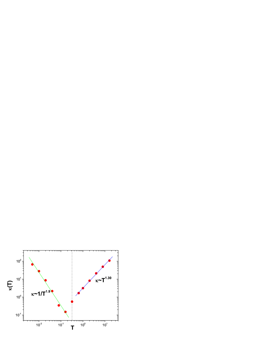
Figure 1: (Color online)Heat conductivity $\kappa$ vs temperature, $T$, for the FK model with lattice length $N=500$. The best fit line is $\kappa\propto T^{-1.9\pm 0.1}$ at the low temperature regime and is $\kappa\propto T^{1.30\pm 0.03}$ at the high temperature regime. The dotted line in the middle is the turning point estimated from the Hamiltonian, $T_{0}=2K/(2\pi)^{2}$, which is $1/\pi$, in the case of $K=2\pi$ in this paper.

From Fig.1 it is clear that the heat conductivity decreases at low temperature region and increases at high temperature region. The turning point can be roughly estimated from the Hamiltonian itself. Here we use the expression of the specific heat again

$$c=\frac{\left<\sum_{i}\left[\frac{p^{2}_{i}}{2}+\frac{1}{2}(x_{i}-x_{i+1})^{2}+\frac{K}{(2\pi)^{2}}(1-\cos{2\pi x_{i}})\right]\right>}{NT}$$ (14)

By definition, $\langle\sum_{i}p^{2}_{i}/2\rangle=NT/2$. At this turning point, we expect the ensemble average of inter particle potential and the on-site potential to be the same value

$$\langle\sum_{i}\frac{1}{2}(x_{i}-x_{i+1})^{2}\rangle=\langle\sum_{i}\frac{K}{(2\pi)^{2}}(1-\cos{2\pi x_{i}})\rangle.$$ (15)

The temperature of the turning point thus can be expressed as

$$T_{0}=\frac{\frac{2K}{(2\pi)^{2}}}{c-1/2}\frac{\langle\sum_{i}(1-\cos{2\pi x_{i}})\rangle}{N}\approx\frac{2K}{(2\pi)^{2}},$$ (16)

where we have used the approximations $c\approx 1$ and $\left<\sum_{i}(1-\cos{2\pi x_{i}})\right>\approx N/2$. With $K=2\pi$ in our numerical calculation, we have $T_{0}=1/\pi$, which is shown as the dotted line in the middle of Fig.1. It is in a good agreement with the numerical calculations.

The $\phi^{4}$ model Another commonly studied model is the $\phi^{4}$ model which has an on-site potential $U(x)=\frac{1}{4}x^{4}$. The coefficient $\alpha=1$. At the low temperature regime, the $\phi^{4}$ model is topologically similar to the FK model. The nonlinear quartic on-site potential in the $\phi^{4}$ model guarantees the particles in stable states, thus the heat conductivity depends on temperature as $\kappa\propto{\cal P}/T$. ${\cal P}$ decreases with temperature because $\gamma$ increases with temperature. Thus the heat conductivity should decrease faster than $\kappa\propto 1/T$ which is consistent with the numerical results in Ref.[9] where $\kappa\propto 1/T^{1.35}$. The high temperature regime of the $\phi^{4}$ model is not in our consideration because it has no energy transport at high temperature limit which is also called anti-continuous or anti-integrable limit[4].

The FPU-$\beta$ model In the FPU-$\beta$ model, $U(x)=0$, and $V(x)=\frac{k}{2}(x_{i}-x_{i+1})^{2}+\frac{\beta}{4}(x_{i}-x_{i+1})^{4}$. We take $k=1$ and $\beta=1$. For the general 1D nonlinear lattices without on-site potential such as the FPU-$\beta$ model, they have total different dynamical properties at low temperature (weak coupling) regime and high temperature (strong coupling) regime. The leading order potential energy is quadratic potential at low temperature regime and quartic potential at high temperature regime. The coefficient $\gamma=0$ for general 1D nonlinear lattices without on-site potential. This property allows us to predict the dependence of heat conductivity more precisely since ${\cal P}$ is a constant. In this case,

$$\kappa\propto\frac{\sqrt{\alpha}}{\epsilon}.$$ (17)

At low temperature regime, the coefficient $\alpha\approx 1$ by definition and the heat conductivity is just proportional to $1/\epsilon$. The dimensionless nonlinearity for the FPU-$\beta$ model is $\epsilon\approx\langle\sum_{i}\frac{1}{4}(x_{i}-x_{i+1})^{4}\rangle/\left<\sum_{i}\frac{1}{2}(x_{i}-x_{i+1})^{2}\right>\propto T$. Thus the heat conductivity $\kappa\propto 1/T$ which is consistent with the numerical results in Ref.[27] and in the Fig.2.

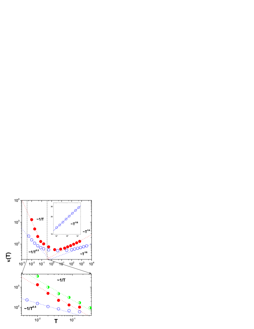
Figure 2: (Color-online)(a) Heat conductivity $\kappa$ vs $T$ for the FPU lattices with $N=2000$. The solid circles are numerical results of the FPU-$\beta$ model. Open circles are that of the FPU-$\alpha$ model with absolute cubic potential where data have been shifted vertically for comparison. The inset is high temperature behavior of the FPU-$\alpha$ model which is actually calculated with parameters $k=0$ and $\alpha^{*}=1$. $k=0$ is equivalent to the high temperature limit. The lower panel is the enlargement of low temperature part. The additional semi circles are from the FPU-$\alpha\beta$ model with cubic and quartic interparticle potential.

At high temperature regime for the FPU-$\beta$ model, the linear potential energy is negligible compared to the nonlinear quartic potential energy. The dimensionless nonlinearity is $\epsilon=\frac{\left<\sum^{N}_{i=1}\frac{1}{4}(x_{i}-x_{i+1})^{4}\right>}{\left<\sum^{N}_{i=1}\frac{1}{2}(x_{i}-x_{i+1})^{2}+\frac{1}{4}(x_{i}-x_{i+1})^{4}\right>}\approx 1$. The heat conductivity only depends on coefficient $\alpha$ at this region as

$$\kappa\propto\sqrt{\alpha}.$$ (18)

The coefficient $\alpha$ can be exactly calculated from the formula in Ref.[16]

$$\alpha = 1+\frac{\int^{\infty}_{0}\phi^{4}e^{-\left(\frac{\phi^{2}}{2}+\frac{\phi^{4}}{4}\right)/T}d\phi}{\int^{\infty}_{0}\phi^{2}e^{-\left(\frac{\phi^{2}}{2}+\frac{\phi^{4}}{4}\right)/T}d\phi}$$ (19)

$$\approx \frac{\int^{\infty}_{0}\phi^{4}e^{-\frac{\phi^{4}}{4T}}d\phi}{\int^{\infty}_{0}\phi^{2}e^{-\frac{\phi^{4}}{4T}}d\phi}=2\frac{\Gamma(\frac{5}{4})}{\Gamma(\frac{3}{4})}T^{1/2},T\rightarrow\infty.$$

Therefore, the heat conductivity at high temperature regime is $\kappa\propto T^{1/4}$. This temperature behavior is consistent with previous results in Ref.[27] and our numerical results in Fig.2.

The FPU-$\alpha$ model We consider the FPU-$\alpha$ model in which $V=\frac{k}{2}(x_{i}-x_{i+1})^{2}+\frac{\alpha^{*}}{3}\left|x_{i}-x_{i+1}\right|^{3}$. We take $k=1$ and $\alpha^{*}=1$. Here the absolute cubic inter particle potential is used to prevent the particles from escaping to infinity which occurs in the usual FPU-$\alpha$ model. At the low temperature regime of the FK model, we have met the case that the heat conductivity doesn’t decrease with temperature as $\kappa\propto 1/T$ which is believed to be universal in solid state physics. Here we present another case that the heat conductivity is not proportional to $1/T$ at the low temperature regime.

Fig.2 shows the numerical results of heat conductivity of this modified FPU-$\alpha$ model as a function of temperature. At the low temperature regime, $\kappa\propto 1/\sqrt{T}$. The dimensionless nonlinearity $\epsilon\approx\left<\sum_{i}\frac{1}{3}\left|x_{i}-x_{i+1}\right|^{3}\right>/\left<\sum_{i}\frac{1}{2}(x_{i}-x_{i+1})^{2}\right>\propto\sqrt{T}$. Thus the prediction derived from our conjecture $\kappa\propto 1/\epsilon\propto 1/\sqrt{T}$ at low temperature regime is in good agreement with the numerical results.

At high temperature regime, the coefficient $\alpha$ is

$$\alpha = 1+\frac{\int^{\infty}_{0}\phi^{3}e^{-\left(\frac{\phi^{2}}{2}+\frac{\phi^{3}}{3}\right)/T}d\phi}{\int^{\infty}_{0}\phi^{2}e^{-\left(\frac{\phi^{2}}{2}+\frac{\phi^{3}}{3}\right)/T}d\phi}$$ (20)

$$\approx \frac{\int^{\infty}_{0}\phi^{3}e^{-\frac{\phi^{3}}{3T}}d\phi}{\int^{\infty}_{0}\phi^{2}e^{-\frac{\phi^{3}}{3T}}d\phi}=3^{1/3}\Gamma\left(\frac{4}{3}\right)T^{1/3}.$$

The heat conductivity should depend on temperature as $\kappa\propto\sqrt{\alpha}\propto T^{1/6}$. The numerical results in Fig.2 confirm this prediction. For the general realistic solids, the inter particle potential can always be expanded as a polynomial form. However, the first order nonlinear potential is cubic where particles will escape to infinity. Particles are more likely to approach the stable states governed by the next order nonlinear potential: quartic potential. This might be the reason that the realistic solids have the universal behavior ($\kappa\propto 1/T$) experimentally at this regime. To check this in 1D we calculate the temperature dependence of heat conductivity of the FPU-$\alpha\beta$ model which has both cubic and quartic inter particle potential besides the harmonic inter particle potential, namely, $V(x_{i},x_{i+1})=\frac{k}{2}(x_{i}-x_{i+1})^{2}+\frac{\alpha^{*}}{3}(x_{i}-x_{i+1})^{3}+\frac{\beta}{4}(x_{i}-x_{i+1})^{4}$ (with $k=1$, $\alpha^{*}=1$, $\beta=1$) and find the temperature dependence of $\kappa$ is more like that of FPU-$\beta$ model (lower panel of Fig.2).

Finally we discuss the possible experiment to verify our conjecture. From the computer simulations we can see that eventually the nonlinearity will cause the heat conductivity to bend upward as the temperature increases. It is worthwhile to point out that the $\phi^{4}$ model does not show this property because it cannot model realistic solids in the high temperature regime. It is not physical to make the substrate on-site potential larger than the interparticle potential which binds the atoms together. The reason we cannot observe this kind of temperature dependence of heat conductivity in realistic solids at room temperature is that the strength of nonlinearity in them is too weak. The realistic solids just start melting before the nonlinearity dominates the transport. However, with nano technology we can build the 1D sample attached to a substrate to demonstrate this counter-intuitive temperature behavior of heat conductivity at room temperature caused by nonlinearity. Now we consider the proposed lattice model with real physical units:

$$H=\sum^{N}_{i=1}\left[\frac{p^{2}_{i}}{2m}+\frac{1}{2}m\omega^{2}(x_{i+1}-x_{i})^{2}+U(x_{i})\right]$$ (21)

where $m$ is the mass of atom, $\omega$ is the oscillation frequency, and $U(x_{i})$ the weak substrate on-site potential with strength $A$ which can be controlled by experiment. As we have discussed above, this on-site potential $U(x_{i})$ does not need to be the FK like potential. $U(x_{i})$ can be any kind of on-site potential with strong nonlinearity. Here the “strong” means the linear part inside $U(x_{i})$ is small compared with the nonlinear part. If the magnitude of this on-site coupling strength is $A$, then using the same analysis we have used for the FK model, the heat conductivity should increase with temperature after

$$T_{0}=\frac{2A}{k_{B}}\,\,\,\,(Kelvin),$$ (22)

and we predict the increase is larger than the linear increase with temperature. To observe this classical behavior explicitly, we must lie outside of the quantum regime where the increase of heat conductivity is mostly caused by the increase of specific heat with temperature. Finally, we must emphasize that the key point for this experiment is the substrate on-site potential with “strong” nonlinearity.

In summary, we have found via computer simulation the strong correlation between the temperature dependence of heat conductivity and the strength of nonlinearity in 1D nonlinear lattices. In the effective phonon theory of heat conduction, we conjecture that the mean-free-path of effective phonon is inversely proportional to the strength of dimensionless nonlinearity. The predictions from this conjecture are consistent with the numerical results in several very general 1D nonlinear lattices with and without on-site potential. We found the temperature dependence of heat conductivity $\kappa\propto 1/T$ is not universal for the model of harmonic lattice with a small nonlinear perturbation. The temperature dependence of heat conductivities in the commonly studied FK and FPU models are explained by our theory at both weak and strong coupling regimes consistently. We have also proposed possible experiment to verify our conjecture.

- [1] E. Fermi, J. Pasta, S. Ulam and M. Tsingou, Los Alamos preprint LA-1940 (1955).
- [2] J. Ford, Phys. Rep. 213, 271 (1992) and the references therein.
- [3] N. Zabusky and M. Kruskal, Phys. Rev. Lett. 15, 240 (1965).
- [4] S. Flach, C. R. Willis, Phys. Rep. 295, 181 (1998) and the references therein.
- [5] D. Campbell, S. Flach, Y. Kivshar, Physics Today, 43 (2004) and the references therein.
- [6] F. Bonetto et al., in Mathematical Physics 2000, edited by A. Fokas et al. (Imperial College Press, London, 2000), p.128; S. Lepri, R. Livi and A. Politi, Phys. Rep. 377, 1 (2003); and the references therein.
- [7] B. Hu, B. Li and H. Zhao, Phys. Rev. E 57, 2992 (1998).
- [8] B. Hu, B. Li and H. Zhao, Phys. Rev. E 61, 3828 (2000).
- [9] K. Aoki and D. Kusnezov, Phys. Lett. A 265, 250 (2000).
- [10] S. Lepri, R. Livi and A. Politi, Phys. Rev. Lett. 78, 1896 (1997).
- [11] S. Lepri, R. Livi and A. Politi, Europhys. Lett. 43, 271 (1998).
- [12] A. Pereverzev, Phys. Rev. E 68, 056124 (2003).
- [13] O. Narayan and S. Ramaswamy, Phys. Rev. Lett. 89, 200601 (2002).
- [14] J.-S Wang and B Li, Phys. Rev. Lett, 92, 074302 (2004); Phys. Rev. E 70, 021204 (2004).
- [15] B. Li and J. Wang, Phys. Rev. Lett. 91, 044301 (2003); 92, 089402 (2004); B. Li, J. Wang, L. Wang and G. Zhang, Chaos 15, 015121 (2005).
- [16] N. Li, P. Tong and B. Li, Europhys. Lett. 75, 49 (2006).
- [17] M. Terraneo, M. Peyrard and G. Casati, Phys. Rev. Lett. 88, 094302 (2002).
- [18] B. Li, L. Wang and G. Casati, Phys. Rev. Lett. 93, 184301 (2004).
- [19] B. Li, J. Lan and L. Wang, Phys. Rev. Lett. 95, 104302 (2005).
- [20] B. Hu, L Yang, and Y Zhang, Phys. Rev. Lett. 97, 124302(2006).
- [21] J.-H Lan and B. Li, Phys. Rev. B 74, 214305 (2006).
- [22] B. Hu and L. Yang, Chaos 15, 015119 (2005).
- [23] B. Li, L. Wang and G. Casati, Appl. Phys. Lett. 88, 143501 (2006).
- [24] C. W. Chang, D. Okawa, A. Majumdar and A. Zettl, Science 314, 1121 (2006).
- [25] C. Kittel, Introduction to Silid State Physics (Seventh Edition, Wiley)
- [26] K. Huang, Statistical Mechanics (Second Edition, Wiley)
- [27] K. Aoki and D. Kusnezov, Phys. Rev. Lett. 86, 4029 (2001).