Rabi oscillations in a quantum dot-cavity system coupled to a non-zero temperature phonon bath

Abstract

We study a quantum dot strongly coupled to a single high-finesse optical microcavity mode. We use a rotating wave approximation method, commonly used in ion-laser interactions, tegether with the Lamb-Dicke approximation to obtain an analytic solution of this problem. The decay of Rabi oscillations because of the electron-phonon coupling are studied at arbitrary temperature and analytical expressions for the collapse and revival times are presented. Analyses without the rotating wave approximation are presented by means of investigating the energy spectrum.

I Introduction

Semiconductor quantum dots (QD) have emerged as promising candidates for studying quantum optical phenomena feng . In particular, cavity quantum electrodynamics (CQED) effects can be investigated using a single QD embedded inside a photonic nano-structure kiraz . One of the most fundamental systems in CQED is an atom interacting with a quantized field plk , such a system has been an invaluable tool to understand quantum phenomena cqedphen as well as for considerations on its applications to realize quantum information cqedinf . Similar systems (in the sense of their treatment, applications, etc.) like trapped ions interacting with lasers trap have shown to be an alternative to develop techniques for quantum information processing ioninf and the study of fundamental effects ionfun . Recent developments in semiconductor nano-technology have shown that excitons in QD constitute yet another two-level system for CQED considerations, and several successful experiments have been carried out wallraff , see also the referee cqd . Contrary to the atom-field interaction where dissipative effects can be fairly overlooked provided the coupling strength between atom and field is sufficiently large compared to the dissipation rate due to cavity losses, the physics of a quantum dot microcavity is enriched by the presence of electro-electron and electron-phonon interactions. Thus, decoherence due to phonons may imply fundamental limitations to quantum information processing on quantum dot CQED wuerger . Here, we would like to analyze the effects of electron-phonon interactions on electron-hole-photon Rabi oscillations in cavity QED.

As in Ref. wilson ; chinese , we will not apply the Born-Markov approximation bm , but will use a different technique for solving this problem. In particular we will make use of techniques commonly applied in ion-laser interactions. It relies on the rotating wave approximation RWA, and within this and the Lamb-Dicke approximation the Hamiltonian becomes diagonal with respect to the phonon subsystem, which is shown in sec. II. In the validity regime of the RWA, the decoherence effect on the inversion, due to the phonon bath, is analyzed in sec. III and analytical expressions for the collapse and revival times are given. The zero temperature situation has been investigated in chinese , while here we study the effects due to zero as well as non-zero temperatures (causing the collapse of the revivals), and also how different phonon mode structures affect the decoherence. A different method to treat the non-zero temperature case was discussed in non-zero , where the collapse time is obtained numerically. The dynamics beyond the rotating wave approximation, shortly studied here in sec. IV, becomes highly complex as can be seen from the energy spectrum. In what sense the phonon decoherence could be used as a possible resource for various applications is briefly mentioned in the concluding remarks.

II The model

We assume a simple two-level model for the electronic degrees of freedom of the QD, consisting of its ground state $|g\rangle$ and the lowest energy electron-hole (exciton) state $|e\rangle$, with the Hamiltonian wilson ($\hbar=1$)

$$\begin{array}[]{lll}\hat{H}&=&\displaystyle{\omega_{eg}\hat{\sigma}_{ee}+\omega\hat{a}^{\dagger}\hat{a}+g(\hat{a}^{\dagger}\hat{\sigma}_{-}+\hat{\sigma}_{+}\hat{a})}\\ \\ &&\displaystyle{+\hat{\sigma}_{ee}\sum_{k}\lambda_{k}(\hat{b}_{k}^{\dagger}+\hat{b}_{k})+\sum_{k}\omega_{k}\hat{b}_{k}^{\dagger}\hat{b}_{k}}.\end{array}$$ (1)

Here $\hat{\sigma}_{+}=|e\rangle\langle g|$, $\hat{a}$ and $\hat{b}_{k}$ are the annihilation operators for the cavity mode and the $k$th phonon mode, respectively. By transforming to a rotating frame, with frequency $\omega$

$$\hat{\cal{H}}\!=\!\Delta\hat{\sigma}_{ee}+g(\hat{a}^{\dagger}\hat{\sigma}_{-}+\hat{\sigma}_{+}\hat{a})+\hat{\sigma}_{ee}\!\!\sum_{k}\!\lambda_{k}(\hat{b}_{k}^{\dagger}+\hat{b}_{k})+\!\sum_{k}\!\omega_{k}\hat{b}_{k}^{\dagger}\hat{b}_{k}$$ (2)

where $\Delta=\omega_{eg}-\omega$ is the detuning. The transformation wuerger ; duke

$$\hat{T}=\prod_{k}e^{\hat{\sigma}_{ee}\frac{\lambda_{k}}{\omega_{k}}(\hat{b}_{k}^{\dagger}-\hat{b}_{k})}$$ (3)

is used to obtain the Hamiltonian $\hat{\cal{H}}_{T}=\hat{T}\hat{\cal{H}}\hat{T}^{\dagger}$

$$\hat{\cal{H}}_{T} = \left(\Delta-\Delta_{\eta}\right)\hat{\sigma}_{ee}+\sum_{k}\omega_{k}\hat{b}_{k}^{\dagger}\hat{b}_{k}$$

$$+ g\left[\hat{a}^{\dagger}\hat{\sigma}_{-}\prod_{k}\hat{D}_{\hat{b}}\left(\eta_{k}\right)+\hat{\sigma}_{+}\hat{a}\prod_{k}\hat{D}_{\hat{b}}^{\dagger}\left(\eta_{k}\right)\right],$$

with $\eta_{k}=\lambda_{k}/\omega_{k}$, $\Delta_{\eta}=\sum_{k}\omega_{k}\eta_{k}^{2}$ is the so-called polaron shift duke and $\hat{D}_{\hat{b}}(\eta_{k})=\exp\left(\eta_{k}\hat{b}^{\dagger}-\eta_{k}^{*}\hat{b}\right)$. For simplicity we look at the case $\Delta=\Delta_{\eta}$ to obtain

$$\hat{\cal{H}}_{T}\!=\!g\!\left[\hat{a}^{\dagger}\hat{\sigma}_{-}\!\prod_{k}\!\hat{D}_{\hat{b}}\left(\eta_{k}\right)+\hat{\sigma}_{+}\hat{a}\!\prod_{k}\!\hat{D}_{\hat{b}}^{\dagger}\left(\eta_{k}\right)\right]+\!\sum_{k}\omega_{k}\hat{b}_{k}^{\dagger}\hat{b}_{k}.$$ (5)

Now by transforming to an interaction picture one obtains

$$\hat{H}_{I}\!=\!g\!\left[\hat{a}^{\dagger}\hat{\sigma}_{-}\!\prod_{k}\!\hat{D}_{\hat{b}}\!\left(\eta_{k}e^{-i\omega_{k}t}\right)+\hat{\sigma}_{+}\hat{a}\!\prod_{k}\!\hat{D}_{\hat{b}}^{\dagger}\!\left(\eta_{k}e^{-i\omega_{k}t}\right)\!\right].$$ (6)

The idea is now to apply the RWA on the above Hamiltonian, equivalent to neglecting all rapidly oscillating terms. However, a closer look at (6) indicates that such a procedure is not straightforward. Normally $\omega_{k}=\omega_{0}k$, $k=1,2,3,...$ and expanding the above exponents give several time-independent cross terms leading to a complicated expression. However, it is know that the RWA is highly related to the Lamb-Dicke approximation dong . In the Lamb-Dicke approximation it is assumed that the variations of the exponents are smaller compared to the characteristic length of the phonon harmonic oscillators, typically $\eta_{k}\ll 1$. One finds that in order to fulfill the RWA one normally needs to be in the Lamb-Dicke regime dong . This observation helps us considerably in approximating the above Hamiltonian, since now the cross time-dependent terms arising from different $k$’s vanish as we assume $\eta_{k}\ll 1$. In this case we can perform the RWA separately on each individual exponent to find

$$\hat{H}_{rwa}=\tilde{g}\left[\hat{a}^{\dagger}\hat{\sigma}_{-}\prod_{k}L_{\hat{n}_{k}}(\eta_{k}^{2})+\hat{\sigma}_{+}\hat{a}\prod_{k}L_{\hat{n}_{k}}(\eta_{k}^{2})\right]$$ (7)

where $L_{\hat{n}_{k}}$ are the Laguerre polynomials of order $\hat{n}_{k}$ wine ; moya and $\tilde{g}=g\exp(\xi/2)\equiv g\exp\left(-\sum_{k}\eta_{k}^{2}/2\right)$ is a rescaled Rabi vacuum frequency. We emphasize that to be consistent with the RWA and Lamb-Dicke approximation, only terms up to $\eta_{k}^{2}$ should be considered when the Laguerre polynomials are expanded in the small parameter $\eta^{2}$. This will be done in the following section. The parameter $\xi$ is sometimes referred to as the Huang-Rhys factor hr , and it is usually very small, $\xi\ll 1$, hrsmall ; rabidot but it can become much larger, $\xi\sim 1$, hrbig and then our analysis would break down. The above equation is readily solvable, finding the evolution operator as

$$\hat{U}=\hat{U}_{ee}\hat{\sigma}_{ee}+\hat{U}_{gg}\hat{\sigma}_{gg}+\hat{U}_{eg}\sigma_{-}+\hat{U}_{ge}\sigma_{+},$$ (8)

where

$$\hat{U}_{ee}(t;\hat{n}_{k})=\cos\hat{\Omega}_{k,\hat{n}+1}t,$$ (9)

$$\hat{U}_{ge}(t;\hat{n}_{k})=-i\epsilon\hat{a}\frac{\sin\hat{\Omega}_{k,\hat{n}}t}{\hat{\Omega}_{k,\hat{n}}},$$ (10)

$$\hat{U}_{eg}(t;\hat{n}_{k})=-i\epsilon\hat{a}^{\dagger}\frac{\sin\hat{\Omega}_{k,\hat{n}+1}t}{\hat{\Omega}_{k,\hat{n}+1}},$$ (11)

and

$$\hat{U}_{gg}(t;\hat{n}_{k})=\cos\hat{\Omega}_{k,\hat{n}}t,$$ (12)

with

$$\hat{\Omega}_{\hat{n}_{k}}=\hat{\epsilon}\sqrt{\hat{n}_{k}}=\tilde{g}L_{\hat{n}_{k}}(\eta_{k}^{2})\sqrt{\hat{n}_{k}}.$$ (13)

III Dynamics

Having the evolution operator, we can in principle calculate any properties we want, in particular we look at the Rabi oscillations for the two-levels system This quantity has as well been studied experimentally in quantum dot systems rabidot . By means of the inversion operator $\sigma_{z}=|e\rangle\langle e|-|g\rangle\langle g|$

$$W(t)=Tr\{\rho(t)\sigma_{z}\}$$ (14)

where $\rho(t)=\hat{U}\rho(0)\hat{U}^{\dagger}$ and $\rho(0)$ is the initial density matrix, Rabi oscillations will be analyzed. This initial state is chosen as the fully separable state

$$\rho(0)=\prod_{k}\rho_{k}(0)|0,e\rangle\langle 0,e|$$ (15)

with the QD excited, the cavity mode in vacuum and the phonon modes are all assumed to be in a thermal distribution

$$\rho_{k}(0)\!=\!\sum_{n_{k}=0}^{\infty}\!|c_{n_{k}}|^{2}|n_{k}\rangle\langle n_{k}|\!=\!\sum_{n_{k}=0}^{\infty}\!\frac{\bar{n}_{k}^{n_{k}}}{(\bar{n}_{k}+1)^{n_{k}+1}}|n_{k}\rangle\langle n_{k}|.$$ (16)

The inversion can be written explicitly as

$$W(t)=\sum_{\{n_{k}\}}\prod_{k}|c_{n_{k}}|^{2}\cos\left(2\tilde{g}\prod_{k^{\prime}}L_{n_{k^{\prime}}}(\eta_{k^{\prime}}^{2})t\right),$$ (17)

where the summation goes from 0 to $\infty$ and runs over all modes. For $t=0$ we have $W(0)=1$ as expected, while for $t\neq 0$ the sum will in general differ from 1. Interestingly we note that at zero temperature, $T=0$, $|c_{n_{k}}|=\delta_{n_{k},0}$ for all $k$ and thus; at absolute zero temperature the system Rabi oscillations are intact but with a rescaled frequency chinese . The expression for the inversion can be simplified by taking into account that $\eta\ll 1$ and we therefore expand the Laguerre polynomials

$$L_{n}(\eta^{2})=\!\sum_{m=0}^{n}\left(\begin{array}[]{c}n\\ m\end{array}\right)\frac{\eta^{2m}}{m!}=1\!-\!n\eta^{2}\!+\!\frac{n(n-1)}{4}\eta^{4}\!+\!...\,.$$ (18)

Keeping only zeroth and first order terms in $\eta_{k}^{2}$ in the assumed Lamb-Dicke regime, the inversion can be written, after some algebra, as

$$\begin{array}[]{lll}W(t)&=&\displaystyle{\cos(2\tilde{g}t){\mathcal{R}e}\left(\prod_{k}\frac{1}{\bar{n}_{k}+1-\bar{n}_{k}\mathrm{e}^{-i2\tilde{g}t\eta_{k}^{2}}}\right)}\\ \\ &&\displaystyle{-\sin(2\tilde{g}t){\mathcal{I}m}\left(\prod_{k}\frac{1}{\bar{n}_{k}+1-\bar{n}_{k}\mathrm{e}^{-i2\tilde{g}t\eta_{k}^{2}}}\right)}.\end{array}$$ (19)

In the following we use dimensionless variables such that the quantum dot-cavity coupling $g=1$, but keep it in the formulas for clarity. There are some special cases worth studying separately.

III.1 Single phonon mode

In the simplest case consisting of a single phonon mode characterized by $\eta$ and $\bar{n}$, the inversion (19) simplifies to

$$W(t)=\frac{(\bar{n}+1)\cos(2\tilde{g}t)-\bar{n}\cos\left[2\tilde{g}t(1-\eta^{2})\right]}{(\bar{n}+1)^{2}+\bar{n}^{2}-2\bar{n}(\bar{n}+1)\cos(2\tilde{g}t\eta^{2})}.$$ (20)

The second term oscillates with a slightly shifted frequency compared to the first term causing a collapse of the inversion. When the two competing terms return back in phase, at times

$$t_{rev}^{(1)}=k\frac{\pi}{\tilde{g}\eta^{2}},\hskip 28.45274ptk=1,2,3,...\,,$$ (21)

inversion revivals occur. These are perfect within the small $\eta^{2}$ expansion. For short times $t$, the inversion may be further approximated to give

$$W(t)=\frac{\cos(2\tilde{g}t)}{1+8\bar{n}(\bar{n}+1)\tilde{g}^{2}\eta^{4}t^{2}},\hskip 28.45274pt2\tilde{g}t\eta^{2}\ll 1,$$ (22)

and we conclude that the envelope function, determining the collapse time, is a Lorentzian with width

$$t_{col}^{(1)}=\frac{1}{\sqrt{8\bar{n}(\bar{n}+1)}\tilde{g}\eta^{2}}.$$ (23)

In fig. 1 we display two different examples of the atomic inversion (17). The upper plot (a) has a large average number of phonons; $\bar{n}=40$ and $\eta=0.01$. In the lower plot (B) the number of phonons is instead $\bar{n}=2$ and again $\eta=0.01$. We can conclude that our results confirm that a lower temperature of the reservoir clearly increases the collapse time.

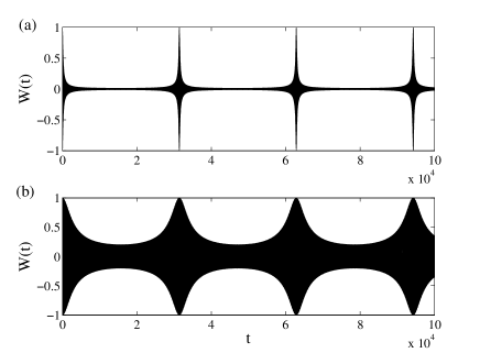
Figure 1: The atomic inversion $W(t)$ as a function of time $t$ for the single mode bath. The dimensionless parameters are $\eta=0.01$ and $\bar{n}=40$ (a) and $\eta=0.01$ and $\bar{n}=2$ (b).

III.2 $N$ identical phonon modes

By studying several identical phonon modes one may see the effect of multi modes in a simple analytic way. Instead of approaching eq. (17) we go back to eq. (5) and let $\eta=\eta_{k}$ and $\omega=\omega_{k}$ for all $k$. Let us introduce a $N\times N$ dimensional unitary operator connecting the boson operators $\hat{b}_{1},\hat{b}_{2},...,\hat{b}_{N}$ with new ones $\hat{c}_{1},\hat{c}_{2},...,\hat{c}_{N}$ such that

$$\hat{c}_{1}=\frac{1}{\sqrt{N}}\sum_{k=1}^{N}\hat{b}_{k}.$$ (24)

The unitary transformed Hamiltonian becomes

$$\hat{\cal{H}^{\prime}}_{T}\!=\!g\!\left[\hat{a}^{\dagger}\hat{\sigma}_{-}\!\hat{D}_{\hat{c}_{1}}\left(\eta\sqrt{N}\right)+\hat{\sigma}_{+}\hat{a}\!\hat{D}_{\hat{c}_{1}}^{\dagger}\left(\eta\sqrt{N}\right)\right]+\!\omega\!\!\sum_{i}\hat{c}_{i}^{\dagger}\hat{c}_{i}.$$ (25)

Thus, the problem relaxes to the single mode case with the scaled Lamb-Dicke parameter $\eta\rightarrow\eta\sqrt{N}$.

III.3 $N$ different phonon modes

In a more realistic model the phonon bath consists of non-identical modes, and depending on the model studied one has different spectral functions $J(\omega)=\sum_{k}\lambda_{k}^{2}\delta(\omega-\omega_{k})$ mahan . For the frequencies of interest here, $J(\omega)$ has a simple power law behaviour power , resulting in a

$$\eta_{k}^{2}=\kappa\omega_{k}^{s},\hskip 28.45274pts=...,-2,-1,0,1,2,...\,,$$ (26)

where $\kappa$ is a constant. The power $s$ depends on matter properties, for example; ohmic damping $J(\omega)\propto\omega$, phonon damping $J(\omega)\propto\omega^{3}$ or impurity damping $J(\omega)\propto\omega^{5}$, but it also depends on system dimensions. We take $\omega_{k}=\omega_{0}k$, $k=1,2,3,...$ such that $\omega_{0}$ determines the frequency spacing, while the thermal phonon distributions are determined from the average phonon numbers

$$\bar{n}_{k}=\left[\exp\left(\frac{\omega_{k}}{\tilde{T}}\right)-1\right]^{-1},$$ (27)

for some scaled temperature $\tilde{T}$. Often a frequency “cut-off” is introduced for the spectral function, but because the vacuum modes do not affect the system dynamics in our case, such a cut-off is not needed. Defining $\gamma_{k}=8\bar{n}_{k}(\bar{n}_{k}+1)\tilde{g}^{2}\eta_{k}^{4}$, and using the same arguments as above the collapse time in the small $\eta^{2}$ expansion is given by

$$\prod_{k}\left(1+\gamma_{k}t_{col}^{2}\right)=2.$$ (28)

By further introducing

$$\begin{array}[]{l}r_{k}=\sqrt{(\bar{n}_{k}+1)^{2}+\bar{n}_{k}^{2}-2\bar{n}_{k}(\bar{n}_{k}+1)\cos(2\tilde{g}t\eta_{k}^{2})},\\ \\ \displaystyle{\theta_{k}=\arctan\left[\frac{\bar{n}_{k}\sin(2\tilde{g}t\eta_{k}^{2})}{\bar{n}_{k}+1-\bar{n}_{k}\cos(2\tilde{g}t\eta_{k}^{2})}\right]}\end{array}$$ (29)

the approximated atomic inversion (19) can be written as

$$W(t)=\frac{\cos(2\tilde{g}t+\theta)}{r},$$ (30)

where $\theta=\sum_{k}\theta_{k}$ and $r=\prod_{k}r_{k}$. In fig. 2, five examples of the atomic inversion are displayed for different powers $s$. Perfect revivals clearly occur for the $s=0$, $s=1$ and $s=2$ cases, while for $s=-2$ and $s=-1$ the revivals are never fully perfect even at long times. This is because if $s=0,1,2,...$ we have $\eta_{k}^{2}=\kappa\omega_{k}^{s}=\kappa\omega_{0}^{s}k^{s}\equiv\eta_{0}^{2}j$ where $j$ is a positive integer, which does not hold if $s=...,-2,-1$. Note that the revivals are a consequence of the non Markovian treatment of the problem; the dynamics is unitary and each phonon mode is considered at the same footing as the cavity mode and the QD themselves. Therefore. also when a large number of different phonon modes are coupled to the QD-cavity system exhibits revivals, however less pronounced.

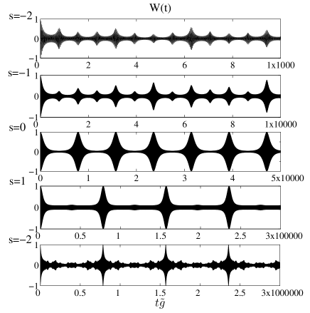
Figure 2: Atomic inversion for different phonon modes obtained from the small $\eta^{2}$ expansion (19). The plots show respectively from top to bottom the cases with powers $s=-2,-1,0,1,2$ of eq. (26). The other parameters are the same for all five cases; $T=0.2$, $\kappa=0.0004$ and $\omega_{0}=0.1$.

IV Beyond the rotating wave approximation

So far all the results have been derived within the RWA and the Lamb-Dicke approximation, which for $g\eta/\omega\ll 1$ is expected to be justified. In this section we calculate the atomic inversion by numerically diagonalyze the truncated Hamiltonian of eq. (5). The size of the Hamiltonian is chosen such that convergence of its eigenstates is guaranteed. We restrict the analysis to the one phonon mode case, which already explains most effects. In the Fock state basis $\{|m\rangle\}$ of the phonon mode, the matrix elements of the Hamiltonian are obtained by using the formula

$$\begin{array}[]{lll}D_{mn}&\equiv&\langle m|\hat{D}(\eta)|n\rangle=\\ \\ &&\displaystyle{=e^{-|\eta|^{2}/2}\eta^{n-m}\!\sqrt{\!\frac{m!}{n!}}L_{m}^{n-m}\!(|\eta|^{2}),\hskip 14.22636ptm\leq n,}\end{array}$$ (31)

where $L_{i}^{j}$ is an associated Laguerre polynomial.

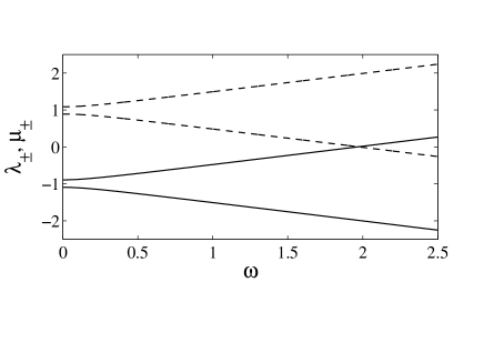
Figure 3: The eigenvalues (33) as function of $\omega$, with $\eta^{2}=0.01$. Dashed curves show $\mu_{\pm}$ and solid curves $\lambda_{\pm}$.

For lowest order truncation of the Hamiltonian, one keeps only a single Fock state of the phonon mode, and the RWA results given above are achieved jonas . In this approximation, when the initial states of the phonon modes are on the form $|c_{n_{k}}|=\delta_{n_{k},n_{k}^{\prime}}$, the combined quantum dot-cavity system persists perfect Rabi oscillations with a rescaled vacuum Rabi frequency $g\rightarrow\tilde{g}\prod_{n_{k}^{\prime}}L_{n_{k}^{\prime}}(\eta_{n_{k}}^{2})$. For zero temperature, all the modes are in the vacuum and the above approximation simply gives a rescaled frequency $g\rightarrow\tilde{g}$, which is the result presented in chinese . Thus, this simple derivation regains the results of chinese , and it is also clear how the approxmation comes about and may be easily extended to non-zero temperature phonon baths. A deeper insight of the approximation (RWA) is gained by increasing the size of the truncated Hamiltonian. In other words, to go beyond the RWA one needs to include more coupling terms arising due to the phonon bath. Considering an initial vacuum phonon mode and including first order corrections to the RWA, the Hamiltonian can be written in matrix form (after an overall shift in energy) as

$$H_{vac}=\left[\begin{array}[]{cccc}\displaystyle{-\frac{\omega}{2}}&0&D_{00}&D_{01}\\ \\ 0&\displaystyle{\frac{\omega}{2}}&D_{01}&D_{11}\\ \\ D_{00}&D_{01}&-\displaystyle{\frac{\omega}{2}}&0\\ \\ D_{01}&D_{11}&0&\displaystyle{\frac{\omega}{2}}\end{array}\right],$$ (32)

with eigenvalues

$$\begin{array}[]{l}\lambda_{\pm}=\displaystyle{-\frac{D_{00}+D_{11}}{2}\!\pm\frac{1}{2}\!\sqrt{\left(D_{00}-D_{11}+\omega\right)^{2}+4D_{01}^{2}}}\\ \\ \mu_{\pm}=\displaystyle{\frac{D_{00}+D_{11}}{2}\!\pm\frac{1}{2}\!\sqrt{\left(D_{00}-D_{11}-\omega\right)^{2}+4D_{01}^{2}}}.\end{array}$$ (33)

These eigenvalues are shown in fig. 3 as function of $\omega$ for fixed $\eta$; $\lambda_{\pm}$ (solid lines) and $\mu_{\pm}$ (dashed lines). The bare curves, $\epsilon_{\pm}^{\lambda}=-D_{ii}\pm\omega/2$ and $\epsilon_{\pm}^{\mu}=D_{ii}\pm\omega/2$, where $i=0,1$, are coupled by the non-RWA term $D_{01}$. This makes the crossings at $\omega=0$ to be avoided, the degeneracies are lifted. Thus, in the RWA, the difference in the values $D_{ii}$ for $i=0,1,2,...$ of the bare energies at $\omega=0$ causes the collapse-revival structure. However, as the non-RWA terms start to dominate the spectrum, the bare energies are no longer proportional to $\pm\omega$ and the full system dynamics will no longer show the nice collapse-revival structure. For which $\omega$ that this non linear behaviour occurs, depends on $g$ and $\eta$. A rough estimate can be derived by assuming that the linear dependence of $\omega/2$ should overrule over the avoided crossing energy difference $2D_{01}$, which after expanding in $\eta$ gives $\omega\gg 4g\eta$. In other words, using our typical parameter values of the previous section, we note that when $\omega<1$ the RWA is likely to break down. For small $\omega$, the eigen energies are very densely spaced, and a small non-RWA correction will couple the different energies in an involved way. The number of states taken into account to correctly describe the dynamics is then growing rapidly, which can be seen in fig. 4 showing the numerically obtained eigenvalues for a $12\times 12$ dimensional (a) and a $22\times 22$ dimensional (b) Hamiltonian. Clearly the more states taken into account, the more complicated energy spectrum.

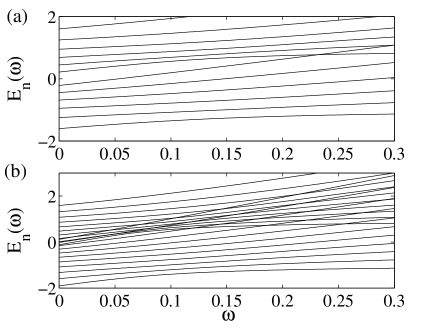
Figure 4: The numerically obtained eigenvalues as function of $\omega$, with $\eta^{2}=0.05$. In (a) the truncated Hamiltonian has size $12\times 12$ and in (b) $22\times 22$. Due to the non-RWA coupling the curve crossings become avoided, which is, however, not seen in the plots of this sice.

Finally, in fig. 5 we give one example of the numerically obtained inversion in a regime where the RWA is not justified. Interestingly, for $\omega\ll 1$ the state $|g\rangle$ (opposite of the initial state) of the QD is more strongly populated, while for increasing $\omega$ the collapse-revival pattern appears and $W(t)\rightarrow 1/2$ in the collapse regions.

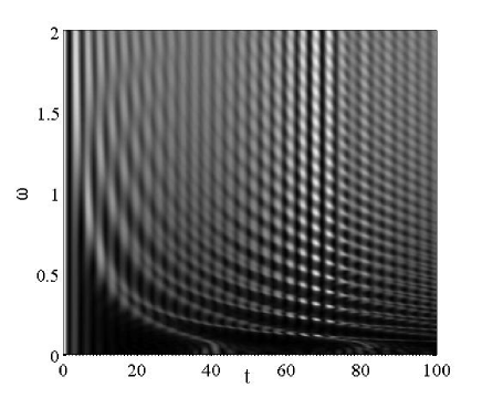
Figure 5: The inversion as function of $\omega$ in the regime where the RWA breaks down. The revivals at $t_{rev}=\pi/\eta^{2}$ build up for increasing $\omega$. Here $\eta^{2}=0.01$ and $\bar{n}=3$.

V Conclusions

We have studied a quantum dot strongly coupled to a single high-finesse optical cavity mode by applying methods usually applied in ion-laser interactions, namely the decomposition of the Glauber displacement operator in Laguerre polynomials. This allowed us to obtain results for the system when it is coupled to a phonon reservoir beyond the Born-Markov approximation. We have studied several cases, including $N$ identical and $N$ different phonon modes, i.e. the case of non-zero temperature. Expressions for the collapse and revival times of the Rabi oscillations have been derived analytically, valid in a large range of parameters.

The analysis is carried out in the resonance condition $\Delta=\Delta_{\eta}$, which in the RWA gives that no population is transferred between the QD and the phonon reservoir. If this resonance is not fulfilled, but other specific types of conditions are (blue or red detuned), one may derive different types of effective Hamiltonians in the RWA, in much resemblance with ion-trap cavity systems plk . Then the effective models will be described by typical generalized two-mode Jaynes-Cummings Hamiltonians, which can often be solved analytically jc . Another assumption made in the derivation is that the cavity mode is initially in vacuum, while for a general initial state each photon states will, just like in the case of the various phonon states, induce different Rabi frequencies affecting the collapse-revival pattern. Such situation may be of interest for state preparation or state measurement and is left for future considerations.

We have also presented a short analysis of the dynamics in the non RWA regime. In this parameter range, the energy spectrum becomes very complex with crossing energy curves, and as the energy spacing between the curves is small for these parameters, many eigenstates of the Hamiltonian must be included in order to correctly describe the dynamics. Non the less, from such an approach it is seen how the RWA results are obtained as a first order correction to the trivial situation, and how higher order terms cause avoided crossings between the energies, and they are therefore no longer proportional to $\pm\omega$ around the crossings which will induce a “breakdown” of the collapse-revival pattern. The higher order terms in such an expansion can be seen as a virtual exchange of phonons jonas2 .

- (1) A. Imamoglu, D. D. Awschalom, G. Burkard, D. P. DiVincenzo, D. Loss, M. Sherwin, and A. Small, Phys. Rev. Lett. 83, 4204 (1999); A. Miranowicz, Ş. K. Özdemir1, Y. Liu, Masato Koashi, N. Imoto1, and Y. Hirayama1, Phys. Rev. A 65, 062321 (2002); M. Feng, I. D’Amico, P. Zanardi, and F. Rossi, Phys. Rev. A 67, 014306 (2003); X. Wang, M. Feng and B.C. Sanders, Phys. Rev. A 67, 022302 (2003).
- (2) J. M. Gérard, B. Sermage, B. Gayral, B. Legrand, E. Costard, and V. Thierry-Mieg, Phys. Rev. Lett. 81, 1110 (1998); C. Becher1, A. Kiraz1, P. Michler1, A. Imamoğlu1, W. V. Schoenfeld, P. M. Petroff, Lidong Zhang, and E. Hu, Phys. Rev. B 63, 121312 (2001); A. Kiraz, C. Reese, B. Gayral, L. Zhang, W.V. Schoenfeld, B.D. Gerardot, P.M. Petroff, E.L. Hu, and A. Imamoglu, J. Opt. B 5, 129 (2003).
- (3) B.W. Shore and P.L. Knight, J. Mod. Optics 40 1195 (1993).
- (4) M. Brune, S. Haroche, J. M. Raimond, L. Davidovich, and N. Zugary, Phys. Rev. A 45, 5193 (1992); M. Brune, E. Hagley, J. Dreyer, X. Maitre, A. Maali, C. Wunderlich, J. M. Raimond, and S. Haroche, Phys. Rev. Lett. 77, 4887 (1996); S. Brattke, B. T. H. Varcoe, and H. Walther, Phys. Rev. Lett. 86, 3534 (2001).
- (5) J. M. Raimond, M. Brune, and S. Haroche, Rev. Mod. Phys. 73, 565 (2001).
- (6) D. Leibfried, R. Blatt, C. Monroe, and D. Wineland, Rev. Mod. Phys. 75, 281 (2003).
- (7) D. Kielpinski, C. Monroe, and D. J. Wineland, Nature 417, 709 (2002).
- (8) D. Leibfried, D. M. Meekhof, C. Monroe, B. E. King, W. M. Itano, and D. J. Wineland, J. Mod Opt. 44, 2485 (1997); C. Roos, T. Zeiger, H. Rohde, H. C. Nagerl, J. Eschner, D. Leibfried, F. Schmidt-Kaler, and R. Blatt, Phys. Rev. Lett. 83, 4713 (1999).
- (9) A. Wallraff, D. I. Schuster, A. Blais, L. Frunzio, R. S. Huang, J. Majer, S. Kumar, S. M. Girvin, R. J. Schoelkopf, Nature 431, 162 (2004); D. I. Schuster, A. A. Houck, J. A. Schreier, A. Wallraff, J. M Gambetta, A. Blaise, L. Frunzio, J. Majer, B. Johnson, M. H. Devoret, S. M. Girvin, R. J. Schoelkppf, Nature 445, 515 (2007); D. Press, S. Gotzinger, S. Reitzenstein, C. Hofmann, A. Löffler, M. Kamp, A. Forchel, and Y. Yamamoto, Phys. Rev. Lett. 98, 117402 (2007); K. Hennessy, A. Badolato, M. Winger, D. Geraee, M. Atature, S. Gulde, S. Fält, E. L. Hu, and A. Imamoglu, Nature 445, 896 (2007); P. J. Leek, J. M. Fink, A. Blais, R. Bianchetti, M. G ppl, J. M. Gambetta, D. I. Schuster, L. Frunzio, R. J. Schoelkopf, A. Wallraff, Science 318, 1889 (2007); D. Englund, A. Faraon, I. Fushman, N. Stoltz, P. Petroff, and J. Vuckovic, Nature 450, 857 (2007).
- (10) G. Khitrova, H. M. Gibbs, M. Kira, S. W. Koch, and A. Scherer, Nature Phys. 2, 81(2006).
- (11) A. Wuerger, Phys. Rev. B 57, 347 (1998).
- (12) I. Wilson-Rae and A. Imamoglu, Phys. Rev. B 65, 235311 (2002).
- (13) W. S. Li, and K. D. Zhu, Chin. Phys. Lett. 20, 1568 (2003); K. D. Zhu, and W. S. Li, Phys. Lett. A 314, 380 (2003).
- (14) H. -P. Breuer, and F. Petruccione, The theory of open quantum systems, (Oxford University Press, 2003); C. W. Gardiner, and P. Zoller, Quantum Noise, (Springer Verlag, 2004).
- (15) K. D. Zhu, Z. J. Wu, X. Z. Yuan, and H. Zheng, Phys. Rev.B 71, 235312 (2005).
- (16) C.B. Duke and G.D. Mahan, Phys. Rev. 139, A1965 (1965).
- (17) W. Dong, T. Hansson, Å. Larson, H. Karlsson, and J. Larson, Submitted to PRA; arXiv:0803.0485.
- (18) D. Leibfried, R. Blatt, C. Monroe, and D. Wineland, Reviews of Modern Physics 75, 281 (2003).
- (19) S. Wallentowitz, W. Vogel and P.L. Knight, Phys. Rev. A 59 531 (1999); S. Wallentowitz adn W. Vogel, Phys. Rev. A 58 679 (1998).
- (20) K. Huang, and A. Rhys, Proc. R. Soc. Lond. A 204, 406 (1950).
- (21) R. Heitz, I. Mukhametzhanov, O. Stier, A. Madhukar, and D. Bimberg, Phys. Rev. Lett. 83, 4654 (1999)
- (22) T. H. Stievater, X. Li1, D. G. Steel, D. Gammon, D. S. Katzer, D. Park, C. Piermarocchi, and L. J. Sham, Phys. Rev. Lett. 87, 133603 (2001); H. Kamada, H. Gotoh, J. Temmyo, T. Takagahara, and H. Ando, Phys. Rev. Lett. 87, 246401 (2001).
- (23) V. Turck, S. Rodt, O. Stier, R. Heitz, R. Engelhardt, U. W. Pohl, D. Bimberg, and R. Steingruber, Phys. Rev. B 61, 9944 (2000).
- (24) M. V. Satyanarayana, P. Rice, R. Vyas, and H. J. Carmichel, J. Opt. Soc. Am. B 6, 228 (1989); S. S. Averbukh, Phys. Rev. A 46, R2205 (1992); P. F. Góra, and C. Jedrzejek, Phys. Rev. A 48, 3291 (1993).
- (25) G. D. Mahan, Many-Particle Physics, (Kluwer, new York 2000).
- (26) A. J. Leggett, S. Chakravarty, A. T. Dorsey, M. P. A. Fisher, A. Garg, and W. Zwerger, Rev. Mod. Phys. 59, 1 (1987).
- (27) J. Larson, and H. Moya-Cessa, J. Mod. Opt. 54, 1497 (2007).
- (28) V. Buzek, G. Drogný, M. S. Kim, G. Adam, and P. L. Knight, Phys. Rev. A 56, 2352 (1997).
- (29) B. W. Shore, and P. L. Knight, J. Mod. Opt. 40, 1195 (1993); A. Messina, S. Maniscalco, and A. napoli, J. Mod. Opt. 50, 1 (2003).
- (30) J. Larson, J. Salo, and S. Stenholm, Phys. Rev. A 72, 013814 (2005).