Magnetic focusing in normal-superconductor hybrid systems: a semiclassical analysis

Abstract

We study a transverse electron-hole focusing effect in a normal-superconductor system. The spectrum of the quasiparticles is calculated both quantum mechanically and in semiclassical approximation, showing an excellent agreement. A semiclassical conductance formula is derived which takes into account the effect of electron-like as well as hole-like quasiparticles. At low magnetic field the semiclassical conductance shows characteristic oscillations due to the Andreev reflection, while at higher fields it goes to zero. These findigs are in line with the results of previous quantum calculations and with the expectations based on the classical dynamics of the quasiparticles.

I Introduction

Investigation of electron-transport properties of normal-superconductor (NS) hybrid nanostructures have attracted considerable interest both experimentally experiments ; Benistant-1:cikk ; Benistant-2:cikk ; Eroms_Ulrich:cikk and theoretically Hoppe_Ulrich:cikk ; Giazotto_Ulrich:cikk ; Fytas:cikk ; Fagas:cikk ; Chtchelkatchev_Burmistrov:cikk in recent years. In NS hybrid systems a crucial physical phenomenon is the Andreev reflectionAndreev whereby an electron incident on a superconductor-normal interface is (partially) retroreflected as a hole into the normal conductor and a Cooper pair is created in the superconductor. The first direct experimental observation of the peculiar property of the Andreev reflection, i.e. that all the velocity components are reversed was achieved by Benistant et al.Benistant-1:cikk ; Benistant-2:cikk using the versatile tool of transverse electron focusing (TEF)Tsoi-review:cikk . The experimental and theoretical investigation of the two-dimensional electron gas using the TEF technique has been pioneered by van Houten et al. Houten_Carlo1:cikk ( see also a recent reviewHouten_Carlo2:cikk discussing these experiments in terms of coherent electron optics).

Recently, Hoppe et al. Hoppe_Ulrich:cikk studied theoretically the interplay of the Andreev reflection and cyclotron motion of quasiparticles at the interface of semi-infinite superconductor and normal regions in a strong magnetic field parallel with the interface. They found that similarly to the normal quantum-Hall systems, edge states are formed which propagate along the NS interface but these ”Andreev” edge states consist of coherent superposition of electron and hole excitations. Therefore they are a new type of current carrying edge states which are induced by the superconducting pair potential. The authors of Ref. Hoppe_Ulrich:cikk, also showed that a semiclassical approximation can give a good agreement for the energy dispersion of the Andreev edge states with the exact results obtained by solving the Bogoliubov-de Gennes equation BdG-eq:konyv (BdG). A clear experimental evidence for the electron and hole transport in edge states have been reported by Eroms et al. Eroms_Ulrich:cikk .

In a disk geometry, it was shown in Refs. sajat-1:cikk ; sajat-2:cikk that such edge states can exist both in the presence but also in the absence of any magnetic field and that the bound state energies calculated semiclassically agree very well with the results obtained from the BdG equation.

Giazotto et al. Giazotto_Ulrich:cikk have extended the study presented in Ref. Hoppe_Ulrich:cikk, by considering the effect of the Zeeman splitting and of the diamagnetic screening currents in the superconductor on the Andreev edge states. Very recently, Fytas et al. Fytas:cikk studied the magnetic field dependence of the transport through a systems consisting of a normal billiard and a superconducting island, while Chtchelkatchev and Burmistrov have also considered the role of the surface roughness in NS junctions Chtchelkatchev_Burmistrov:cikk .

In this work we consider the NS hybrid system depicted in Fig. 1.

Figure 1: The hybrid NS nanostructure that we investigate. It consists of an infinitely long two dimensional ballistic normal conductor of width $W$ coupled to a semi-infinite spin-singlet superconductor region. The conductance is measured between two normal conducting quantum point contacts: an injector (of width $W_{i}$) and a collector (of width $W_{c}$ and at distance $L$ from the injector). The magnetic field $B$ is applied perpendicular to the system (in our calculation $B>0$ corresponds to a field pointing out of the plane of the system).

It is similar to the experimental setup of Ref. Benistant-1:cikk, but in our system the normal conducting region is a two-dimensional electron gas. It is assumed that the quasiparticle transport in the waveguide is ballistic and that the waveguide can act as drain which absorb any quasiparticles exiting to the left of the injector or to the right of the collector.

First, we calculate the eigenstate of such a system where the quantum point contacts are not present, ie we consider a normal waveguide in contact with a superconductor. We show how the interplay of the lateral confinement brought about by the finite width of the lead, the applied magnetic field and the proximity effect gives rise to a rich physics in this system. We calculate the eigenstates of the system by solving the BdG equation and then these exact quantum results are compared with results obtained from semiclassical calculations. As we shall show below the agreement is excellent. We note that the semiclassical approximation we used is applicable in a wider parameter range than the one used in Refs. Hoppe_Ulrich:cikk, ; Giazotto_Ulrich:cikk, for a similar system.

Having obtained the exact eigenstates and their semiclassical approximations, we then turn to the calculation of conductance for the case when the two quantum point contacts, as depicted in Fig. 1, are present. The conductance between the injector and the collector is determined by adopting the method used by van Houten et al. Houten_Carlo1:cikk to describe the TEF in a two dimensional electron gas. In our system however, we have to take into account the dynamics of both the electron and of the hole quasiparticles. Thus, our results on the conductance can be considered as a generalisation of the corresponding semiclassical calculations of Ref. Houten_Carlo1:cikk, .

Recently, the same NS system has been studied numerically sajat-3:cikk using a Green’s function technique sanvito . The influence of the underlying classical dynamics on the conductance has been, however, discussed only qualitatively. Our rigorous semiclassical treatment gives a quantitative analysis of the dependence of the transport on the classical dynamics of quasiparticles.

The rest of the paper is organised as follows. In Section II we present the exact quantum calculations based on the BdG equation. Then in Section III we discuss the results of the semiclassical approximations of the exact quantum calculations.

In Section IV we compare the results of the quantum and of the semiclassical calculations and give the physical interpretation of the results. Section V is devoted to the semiclassical calculation of the conductance between the injector and the collector which is the central result of our paper. Finally, in Section VI we come to our conclusions.

II Quantum calculation

In this section we consider a system consisting of a normal conducting waveguide of width $W$ in contact with a semi-infinite superconducting region. We derive a secular equation solutions of which give the energies of the bound states of the system.

The eigenstates and eigenenergies can be obtained from the BdG equation:

$$\left(\begin{array}[]{cc}H_{0}&\Delta\\ \Delta^{*}&-H_{0}^{*}\end{array}\right)\mathbf{\Psi}(x,y)=E\,\mathbf{\Psi}(x,y),$$ (1)

where $\mathbf{\Psi}$ is a two-component wave function and $H_{0}={\left({\bf p}-e{\bf A}\right)}^{2}/(2m)+V-E_{\rm F}$ is the single-electron Hamiltonian (for simplicity, we assume that the effective mass $m$ and the Fermi energy $E_{\rm F}$ is the same in the N and S regionsnote-1 ). The excitation energy $E$ is measured relative to $E_{\rm F}$. Scattering at the NS interface is modeled by an external potential $V(x)=U_{0}\delta(x)$. Hard wall boundary condition is imposed at the wall of the wave guide which is not adjacent to the superconductor, i.e. $\mathbf{\Psi}(x=W,y)=0$. The bound state energies are the positive eigenvalues $0<E<\Delta$ of the BdG equationBdG-eq:konyv . The superconducting pair potential $\Delta$ can be approximated by a step function $\Delta({\bf r})=\Delta_{0}\Theta(-x)$ without changing the results in any qualitative wayref:andreev_billiards . Owing to the translational symmetry along the $y$ direction it is convenient to chose the Landau gauge for the vector potential: ${\bf A}({\bf r})=B\,{(0,x,0)}^{T}$ (here $T$ denotes the transpose of a vector). Thus, the wave function $\mathbf{\Psi}(x,y)={(\mathbf{\Psi}_{\rm e}(x,y),\mathbf{\Psi}_{\rm h}(x,y))}^{T}$ can be separated and in the N region it reads

$$\mathbf{\Psi^{(N)}}(x,y)=\begin{pmatrix}A_{e}\,\Phi_{\rm e}^{(N)}(x)\\ A_{h}\,\Phi_{\rm h}^{(N)}(x)\end{pmatrix}e^{iky},$$ (2)

where $k$ is the wave number along the $y$ direction and the amplitudes $A_{e,h}$ will be determined from the boundary conditions given below. Substituting $\mathbf{\Psi^{(N)}}(x,y)$ into the BdG equation we find that the function $\Phi^{N}_{e}(x)$ satisfies the following one-dimensional Schrödinger equation:

$$\frac{d^{2}\Phi_{\rm e}^{(N)}(\xi)}{d\xi^{2}}-\left(\frac{1}{4}\xi^{2}+a\right)\Phi_{\rm e}^{(N)}(\xi)=0,$$ (3a)

where

$$\xi=\sqrt{2}\left(\frac{x}{l}-\text{sign}(eB)kl\right),\,\,a=-\left(\frac{E}{\hbar\omega_{\rm c}}+\frac{\nu_{0}}{2}\right).$$ (3b)

Here $l=\sqrt{\hbar/{\left|eB\right|}}$ is the magnetic length, $\omega_{\rm c}=\left|eB\right|/m$ is the cyclotron frequency, and $\nu_{0}=2E_{\rm F}/(\hbar\omega_{\rm c})$ is the filling factor. Equation (3a) is a parabolic cylinder differential equation Abramowitz and its solution can be expressed in terms of the Whittaker functions $U(a,\xi)$ and $V(a,\xi)$:

$$\Phi_{\rm e}^{(N)}(x)=U(a,\xi)-\frac{U(a,\xi_{W})}{V(a,\xi_{W})}\,V(a,\xi),$$ (4)

where $\xi_{W}=\sqrt{2}\left(W/l-\text{sign}(eB)kl\right)$. Note that the function $\Phi_{\rm e}^{(N)}(x)$ satisfies Dirichlet boundary condition at $x=W$. From the BdG equation it follows that for the hole component $\Phi_{\rm h}^{(N)}(x)$ of the wave function the symmetry relation

$$\Phi_{\rm h}^{(N)}(B,E,x)=\Phi_{\rm e}^{(N)}(-B,-E,x)$$ (5)

holds.

The magnetic field is assumed to be screened from the superconducting region, hence the vector potential is taken to be zero (for the case of finite magnetic penetration length see e.g. Ref. Giazotto_Ulrich:cikk, ). Therefore, in the S region the wave function ansatz with eigenenergy $E$ can be written as sajat-1:cikk

$$\!\!\!\!\mathbf{\Psi^{(S)}}(x,y) = \!\!\!\!\left[C_{e}\!\!\begin{pmatrix}\gamma_{e}\\ 1\end{pmatrix}\!\!\Phi_{e}^{(S)}(x)\!+\!C_{h}\!\!\begin{pmatrix}\gamma_{h}\\ 1\end{pmatrix}\!\!\Phi_{h}^{(S)}(x)\right]\!\!e^{iky},$$ (6a)

where

$$\Phi_{e,h}^{(S)}(x) = e^{\pm iq_{e,h}x},$$ (6b)

$$q_{e,h} = k_{\rm F}\sqrt{1-\frac{k^{2}}{k^{2}_{\rm F}}\mp i\eta},$$ (6c)

$\eta=\sqrt{\Delta_{0}^{2}-E^{2}}/E_{\rm F}$, $\gamma_{e,h}=\frac{\Delta_{0}}{E\pm i\sqrt{\Delta_{0}^{2}-E^{2}}}$, and $k_{\rm F}=\sqrt{2mE_{\rm F}}/\hbar$ is the Fermi wave number (the upper/lower signs in the expressions correspond to the electron/hole component). Note that in the S region the wave function $\mathbf{\Psi}^{(S)}(x,y)$ goes to zero for $x\to-\infty$.

The four coefficients $A_{e,h},C_{e,h}$ in Eqs. (2) and (6a) are determined by the the boundary conditions at the NS interfacesajat-1:cikk ; sajat-2:cikk :

$$\begin{split}\big{.}\mathbf{\Psi^{(N)}}\big{|}_{x=0}&=\big{.}\mathbf{\Psi^{(S)}}\big{|}_{x=0},\\ \left.\frac{d}{dx}\left[\mathbf{\Psi^{(N)}}-\mathbf{\Psi^{(S)}}\right]\right|_{x=0}&=\frac{2m}{\hbar^{2}}U_{0}\big{.}\mathbf{\Psi^{(N)}}\big{|}_{x=0},\end{split}$$ (7)

for all $y$ and $k$. The matching conditions shown in Eq. (7) yield a secular equation for the eigenvalues $E$ as a function of the wave number $k$. Using the symmetry relations between the electronic and hole-like component of the BdG eigenspinor given by Eq. (5), the secular equation can be reduced to sajat-1:cikk ; sajat-2:cikk

$$\rm{Im}\left\{\gamma_{e}D_{e}(E,B)\,D_{h}(E,B)\right\}=0,$$ (8a)

where the $$2\times 2 D_{e} D_{h}$$ determinants and are given by

$$D_{e}(E,B) = \left|\begin{array}[]{cc}\Phi_{e}^{(N)}&\Phi_{e}^{(S)}\\ {\left[\Phi_{e}^{(N)}\right]}^{\prime}&Z\Phi_{e}^{(S)}+{\left[\Phi_{e}^{(S)}\right]}^{\prime}\end{array}\right|,$$ (8d)

$$D_{h}(E,B) = D_{e}(-E,-B).$$ (8e)

Here $Z=\left(2m/\hbar^{2}\right)\,U_{0}$ is the normalised barrier strength, and the prime denotes the derivative with respect to $x$. All functions are evaluated at the NS interface ie. at $x=0$. The secular equation derived above is exact in the sense that the usual Andreev approximation is not assumed ref:andreev-approx . An analogous result was found previously sajat-1:cikk ; sajat-2:cikk for NS disk systems.

III Semiclassical approximation

As a first step to calculate the conductance between the injector and collector we should solve the exact quantisation condition (8) which involves evaluation of parabolic cylinder functions. It turns out that for certain parameter ranges this makes the actual numerical calculations rather difficult. However, as we are going to show it in Section IV, for the quasiparticle dispersion relations which will be important in the subsequent analysis, one can obtain excellent approximations using semiclassical methods. The use of the semiclassical approximations makes the numerical calculations much simpler and gives a better understanding of the underlying physics. The semiclassical calculations are based on (i) the WKB approximationBrack:konyv of the functions $\Phi_{e}(x)$, $\Phi_{h}(x)$ [see Eqs. (3a) and (5)] and their derivatives (ii) the Andreev-approximationref:andreev-approx . The approximated wave functions are then substituted into Eq. (8a) to obtain the semiclassical quantisation conditions. The calculations can be carried out in a similar fashion as in Ref. sajat-2:cikk, , therefore in this section and in the next one we only summarise the main results. Throughout the rest of the paper we assume ideal NS interface, ie we set $U_{0}=0$.

Depending on the energy of the electrons (holes) and the applied magnetic field, eight different types of orbits can be distinguished. These orbits, denoted by capital letters $A$ to $H$, are shown in Fig. 2. In the geometrical construction of the classical trajectories we took into account that the chiralities of the electron-like and the hole-like orbits are preserved when electron-hole conversion occurs at the NS interface Giazotto_Ulrich:cikk .

Type $A$ orbits correspond to skipping motion of alternating electron and hole quasiparticles along the NS interface. Neither the electron’s nor the hole’s trajectory hits the wall of the wave guide at $x=W$. This type of orbit was first considered by Hoppe et al. Hoppe_Ulrich:cikk . Type $B$ and $C$ orbits are similar to type A but the either the electron or the hole can now reach the wall of the wave guide at $x=W$. In case of type $D$ orbits the electrons and holes bounce both at the wall of the wave guide and at the NS interface, while for type $E$ ($G$) orbits the quasiparticles are moving on cyclotron orbits. Type $F$ ($H$) is the familiar edge state of the integer quantum Hall systems. The electrons (holes) are moving on skipping orbits along the wall of the wave guide at $x=W$.

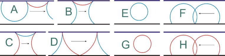
Figure 2: Classification of the possible orbits. The blue/red lines correspond to electron/hole trajectory segments. The black arrows show the direction of the group velocity (cf. the slope of the dispersion curves in Figs. 3 and 4) for a magnetic field pointing out of the plane.

The semiclassical quantisation condition for the orbits shown in Fig. 2 can be written in the following simple form:

$$N(E)=n+\mu,\qquad\text{for}\quad n\in\mathbb{Z},$$ (9a)

where $$N(E) S_{e}(\tau_{+}^{e},\tau_{-}^{e}) S_{h}(\tau_{+}^{h},\tau_{-}^{h}) \mu S_{e,h}$$ can be expressed in terms of the (dimensionless) classical action integrals , (see Table 1) for different types of orbits and is the corresponding Maslov index. The actions are given by the following equations:

$$S_{e}(\tau_{+}^{e},\tau_{-}^{e}) = 2\left(\Theta_{\rm e}(\tau_{+}^{e})-\Theta_{\rm e}(\tau_{-}^{e})\right),$$ (9b)

$$S_{h} = S_{e}(-E-B),$$ (9c)

$$\Theta_{\rm e}(x) = \frac{\left|eB\right|}{2\pi\hbar}\int\limits\sqrt{R_{\rm e}^{2}-\left(x-X\right)^{2}}\;{\rm d}x$$ (9d)

$$= \frac{E+E_{\rm F}}{2\pi\hbar\omega_{\rm c}}\left[\arcsin\frac{x-X}{R_{\rm e}}\right.$$

$$+\left.\frac{1}{2}\,\sin\left(2\arcsin\frac{x-X}{R_{\rm e}}\right)\right],$$

$$\Theta_{\rm h} = \Theta_{\rm e}(-E,-B).$$ (9e)

Here the cyclotron radii $$R_{\rm e,h} \tau^{e,h}_{\pm}$$ and the classical turning points for electrons and holes are given by

$$R_{\rm e,h} = R_{c}\sqrt{1\pm E/E_{\rm F}},\quad R_{c}=k_{\rm F}l^{2},$$ (9f)

$$\tau^{e}_{+} = \min\left\{W,X+R_{e}\right\},$$ (9g)

$$\tau^{e}_{-} = \max\left\{0,X-R_{e}\right\},$$ (9h)

$$\tau^{h}_{\pm} = \tau^{e}_{\pm}(-B,-E),$$ (9i)

where $X={\rm sign}(eB)kl^{2}$ is the guiding center coordinate. Finally, contributions to the Maslov index of a given type of orbit come from the collisions with the wall of the waveguide, from the collisions with the superconductor (Andreev reflections), and from the caustics of the electron (hole) segments of the orbit (see Table.1).

type of orbit	$N(E)$	$\mu$	conditions for orbits
$A$	$S_{e}(\tau_{+}^{e},\tau_{-}^{e})-S_{h}(\tau_{+}^{h},\tau_{-}^{h})$	$\frac{1}{\pi}\arccos\left(\frac{E}{\Delta}\right)$	$\tau_{+}^{e},\tau_{+}^{h}<W,\quad\tau_{-}^{e},\tau_{-}^{h}=0$
$B$	$S_{e}(\tau_{+}^{e},\tau_{-}^{e})-S_{h}(\tau_{+}^{h},\tau_{-}^{h})$	$-\frac{3}{4}+\frac{1}{\pi}\arccos\left(\frac{E}{\Delta}\right)$	$\tau_{+}^{e}=W,\quad\tau_{+}^{h}<W,\quad\tau_{-}^{e},\tau_{-}^{h}=0$
$C$	$S_{e}(\tau_{+}^{e},\tau_{-}^{e})-S_{h}(\tau_{+}^{h},\tau_{-}^{h})$	$-\frac{1}{4}+\frac{1}{\pi}\arccos\left(\frac{E}{\Delta}\right)$	$\tau_{+}^{e}<W,\quad\tau_{+}^{h}=W,\quad\tau_{-}^{e},\tau_{-}^{h}=0$
$D$	$S_{e}(\tau_{+}^{e},\tau_{-}^{e})-S_{h}(\tau_{+}^{h},\tau_{-}^{h})$	$\frac{1}{\pi}\arccos\left(\frac{E}{\Delta}\right)$	$\tau_{+}^{e},\tau_{+}^{h}=W,\quad\tau_{-}^{e},\tau_{-}^{h}=0$
$E$	$S_{e}(\tau_{+}^{e},\tau_{-}^{e}))$	$\frac{1}{2}$	$\tau_{+}^{e}<W,\quad\tau_{-}^{e}>0$
$F$	$S_{e}(\tau_{+}^{e},\tau_{-}^{e})$	$-\frac{1}{4}$	$\tau_{+}^{e}=W,\quad\tau_{-}^{e}>0$
$G$	$-S_{h}(\tau_{+}^{h},\tau_{-}^{h})$	$-\frac{1}{2}$	$\tau_{+}^{h}<W,\quad\tau_{-}^{h}>0$
$H$	$-S_{h}(\tau_{+}^{h},\tau_{-}^{h})$	$-\frac{3}{4}$	$\tau_{+}^{h}=W,\quad\tau_{-}^{h}>0$

Table 1: $N(E)$ related to the actions defined in Eq. (9), and the conditions for the possible orbits shown in Fig 2.

IV Dispersion relation and the phase diagram for NS systems

In this section we compare the numerical results obtained from the exact and from the semiclassical calculations outlined in Sections II and III. The above discussed classical orbits can exist in different parameter ranges, depending on the strength of the magnetic field, on the Fermi energy and on the width of the normal lead. It is convenient to use the following dimensionless parameters: $\nu_{0}$, $\Delta_{0}/\hbar\omega_{\rm c}$, $k_{\rm F}W$ and $R_{c}/W$. Figures 3 and 4 show comparisons of the exact quantum calculations with the semiclassical results for the dispersion relation of the quasiparticles.

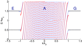
Figure 3: The energy spectrum obtained from Eqs. (8) (solid/blue line) and (9) (red crosses) as a function of $k$. The parameters are $\nu_{0}=40$, $\Delta_{0}/\hbar\omega_{\rm c}=2$, $k_{\rm F}W=106.7$ and $R_{c}/W=0.375$. In the semiclassical calculations only the orbits of type $A$, $E$ and $G$ need to be taken into account.

Figure 4: The same as in Fig. 3 with parameters $\nu_{0}=160$, $\Delta_{0}/\hbar\omega_{\rm c}=8$, $k_{\rm F}W=106.7$ and $R_{c}/W=1.5$. In the semiclassical calculations the orbits of type $B$, $C$, $D$, $F$ and $H$ are involved.

In case of Fig. 3 the magnetic field is strong so that the cyclotron radius is smaller than the width of the waveguide. One expects therefore that type A orbits and Landau levels (corresponding to orbits of type $E$ and $G$) would appear in the spectrum. One can see that this is exactly the case, the Landau levels appearing as dispersionless states. The agreement between the quantum and semiclassical calculations is excellent except in the transition regime between type A and type E (G) orbits. In case of Fig. 4 the magnetic field is weaker than for Fig. 3 and therefore $R_{c}$ is now larger than $W$. No Landau levels appear and the dispersion relation can be well approximated semiclassically using orbits of type $B$, $C$, $D$, $F$ and $H$.

Whether or not a given type of classical orbit is allowed for a certain set of parameter values depends on the positions of the turning points with regard to the wall of the wave guide and to the NS interface. The conditions for each type of orbits are summarised in Table 1. The turning points depend [see Eqs. (9f) – (9i)] on the width of the lead $W$, on the Fermi wavenumber $k_{\rm F}$, on the magnetic field (or equivalently, on the cyclotron radius $R_{c}$), and on the wave number $k$. In an experiment the former two parameters would be fixed, $R_{c}$ could be varied by varying the magnetic field, while the wave number $k$ of the injected electrons would be uniformly distributed if there are many open channels in the quantum point contact. For a given $W$ and $k_{\rm F}$, ie for a given experimental sample, one can then draw a ”phase diagram”, which shows the allowed types of classical orbits as a function of $R_{c}$ and $k$. An example of such a diagram is shown in Fig. 5.

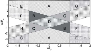
Figure 5: The phase diagram of the allowed type of orbits as a function of $R_{c}$ and $k$. The white regions are classically forbidden. The energy of the quasiparticles is $E=0$.

Note that the weak energy dependence of the turning points translates into a similarly weak energy dependence of the phase diagram. Thus for Fig. 5 we have chosen $E=0$. The white regions are classically forbidden, as no classical orbit can be realized for these parameter values.

V Coherent electron-hole focusing

Having obtained the spectrum of the quasiparticles, we have now all the necessary information to calculate the conductance between the injector and collector for the NS system shown in Fig. 1. For $W_{i},\,\,W_{c}\ll\lambda_{F}$ the calculations in principle could be carried out using the exact results of Section II. However, this would involve evaluations of the Whittaker functions [see Eq. (4)] which would render the numerical calculations rather difficult. Therefore we calculate the conductance semiclassically, adopting and generalising the method of Ref. Houten_Carlo1:cikk, to account for all types of current carrying modes. Namely, the dynamics of hole type quasiparticles created by Andreev reflections also needs to be taken into consideration. We assume that $W_{i},W_{c}\ll R_{c}$ meaning that the angular distribution of the injected electrons is not perturbed by the magnetic field.

In classical picture injected electrons having orbits of type B or D can contribute to the conductance, since only these orbits can reach the collector (note that for type F orbit the group velocity points in the $-y$ direction). Assuming that the wave function in the wave guide is unperturbed by the presence of the collectorHouten_Carlo1:cikk , the current at the collector is given by

$$I_{\rm c}=\varepsilon\left(\left|\frac{\partial\mathbf{\Psi}_{\rm e}}{\partial x}(W,L)\right|^{2}-\left|\frac{\partial\mathbf{\Psi}_{\rm h}}{\partial x}(W,L)\right|^{2}\right),$$ (10)

where $\varepsilon$ is an yet undetermined parameter but will drop out when we calculate the conductance. This expression is the generalisation of Eq. (16) in Ref. Houten_Carlo1:cikk, by including the contribution of the holes. In WKB approximation the wave function $\mathbf{\Psi^{(N)}}(x,y)=(\mathbf{\Psi}_{\rm e}(x,y),\mathbf{\Psi}_{\rm h}(x,y))^{T}$ in the wave guide is the sum over all classical trajectories from the injector to the point $(x,y)$ of an amplitude factor times a phase factor. As in Ref. Houten_Carlo1:cikk, we transform the sum over trajectories into a sum over modes using saddle point integration. Finally, we find

$$\frac{\partial\mathbf{\Psi}_{\rm e}}{\partial x}(W,L)=$$ (11a)

$$-2ik_{\rm F}\sum_{\scriptstyle n\atop\scriptstyle K=B,D}\sqrt{2\pi i\!\left(\!\!\frac{\partial^{2}S^{K}_{e}(p_{n})}{\partial p_{n}^{2}}\!\!\right)^{-1}}A_{p_{n}}^{K}e^{ik_{n}^{K}L-i\pi}\cos\alpha_{n}^{K},$$

and

$$\frac{\partial\mathbf{\Psi}_{\rm h}}{\partial x}(W,L)=$$ (11b)

$$-2ik_{\rm F}\sum_{n}\sqrt{2\pi i\!\left(\!\!\frac{\partial^{2}S^{D}_{h}(p_{n})}{\partial p_{n}^{2}}\!\!\right)^{-1}}A_{p_{n}}^{D}e^{ik_{n}^{D}L-i\pi}\cos\alpha_{n}^{D}.$$

For simplicity, here we give the definitions of the different terms appearing in the above expressions only for electrons having type $B$ orbits. For holes and for type $D$ orbits similar expressions were derived but are not presented here. The wave numbers $k_{n}$ of the excited modes (for a given magnetic field) can be obtained from the dispersion relation by solving the equation $E(k_{n},R_{c})=E$. The amplitudes $A^{B}_{p_{n}}$ of the modes related to type $B$ of orbits are given by

$$A^{B}_{p_{n}}=\sqrt{\frac{I_{i}\cos\alpha_{n}}{2v_{\rm F}L}\,\frac{d(\alpha_{n})}{d^{\prime}(\alpha)|_{\alpha=\alpha_{n}}}},$$ (12)

where $I_{i}$ is the current injected from the injector, $v_{\rm F}=\hbar k_{\rm F}/m$ is the Fermi velocity of the quasiparticles and the prime denotes derivation with respect to $\alpha$. Here $\alpha$, $\alpha_{n}$ and $d(\alpha_{n})$ are defined in the following way: the distance between two subsequent bouncing at the wall of the wave guide for an electron injected at angle $\alpha$ (measured from the $y$ axis) is $d(\alpha)=4\sqrt{R_{c}^{2}-{\left(W-R_{c}\sin\alpha\right)}^{2}}-2R_{c}\cos\alpha$. Then $p=L/d(\alpha)$ is the number of bounces between the injector and collector. The angle $\alpha$ can also be expressed by $\sin\alpha=(W-X)/R_{c}$ and it can be related to the wave number $k_{n}$ of the modes. Since for mode $k_{n}$ the guiding centre coordinate is $X={\rm sign}(eB)k_{n}l^{2}$, we have $\sin\alpha_{n}=W/R_{c}-{\rm sign}(eB)k_{n}/k_{\rm F}$ (because $R_{c}=k_{\rm F}l^{2}$), and then $p_{n}=L/d(\alpha_{n})$. Finally, $S^{B}_{e,\,(h)}(p_{n})$ is related to the action of electrons (holes) calculated from the injector to the collector. In case of type $B$ orbits the summation over $n$ includes only those modes for which the group velocity $\partial E(k)/\partial(\hbar k)$ is positive, i.e the mode propagates from the injector to the collector. (Note that the group velocity is basically given by the slope of the curves in Fig.4).

The conductance $G(E,R_{c})$ between the injector and the collector is $G=I_{i}/V_{c}$, where $V_{c}$ is the collector voltage. Taking into account Eq. (10) it can be calculatedHouten_Carlo1:cikk as

$$V_{\rm c}=\varepsilon\left(\frac{\left|\frac{\partial\Psi_{\rm e}}{\partial x}(W,L)\right|^{2}}{G_{\rm e}}-\frac{\left|\frac{\partial\Psi_{\rm h}}{\partial x}(W,L)\right|^{2}}{G_{\rm h}}\right).$$ (13)

Here $G_{e}$ ($G_{h}$) is the conductance of the point contact of the collector for electrons (holes). It is estimated by Eq. (17) in Ref. Houten_Carlo1:cikk, . Since both $G_{e}$ and $G_{h}$ are proportional to the parameter $\varepsilon$, it drops out from $V_{c}$. Similarly, the injected current $I_{i}$ drops out from $G(E,R_{c})$ since the derivatives of the wave functions in (11) are proportional to $\sqrt{I_{i}}$ through the amplitudes $A_{p_{n}}$.

Equations (10), (11) and (13) allow us to calculate the conductance semiclassically as a function of the energy of quasiparticles and of the magnetic field. This is the main result of our paper. An example is shown in Fig. 6.

Figure 6: The conductance $G$ for low magnetic fields at $E=0$. Inset: the conductance for stronger magnetic fields. We used $k_{\rm F}W=26.7$.

One can clearly see that for small magnetic fields ($W/R_{c}<0.4$) the conductance is a rapidly oscillating function of the magnetic field and can also be negative. The first observation is the consequence of the constructive interference of many coherently excited modes (edge states). Similar effect was found by van Houten et al. Houten_Carlo1:cikk ; Houten_Carlo2:cikk . The fact that the conductance can be negative is a consequence of the hole-like excitations in the hybrid NS system. Indeed, at low magnetic fields (large $R_{c}$) an injected electron will undergo one or more Andreev reflections and it can happen (see type D orbits) that a hole will arrive to the collector resulting in negative conductance. This is the so called Andreev-drag effectsajat-3:cikk . The heights of the positive peaks are comparable with those of the negative ones, indicating that it can be a robust effect. This observation is in line with the findings of Ref. Benistant-1:cikk, and also with the results of Ref. sajat-3:cikk, where an exact (numerical) quantum calculation has been performed for the same system.

The use of WKB approximation means that our results should be accurate at low magnetic fields when a large number of edge states are populated. Nevertheless, we find that this method, at least qualitatively, also describes the regime of high magnetic fields. Namely, from the inset of Fig. 6 one can see that increasing the magnetic field the conductance decreases and rapidly goes to zero for $W/R_{c}>1.5$. This can be understood from classical considerations. Increasing the magnetic field the cyclotron radius decreases and at a certain value of the field we have $2R_{c}<W$ meaning that no injected electron can hit the superconductor and undergo Andreev reflections. Instead, the electrons move to the left skipping along the wall of the wave guide (type $F$ of orbits) and eventually they leave the system without reaching the collector, ie the conductance becomes zero. According to our semiclassical calculations, for a system with $k_{\rm F}W=26.7$ as in case of Fig.6 the last current-carrying mode disappears when $W/R_{c}\gtrsim 1.8$, in broad agreement with the classical picture.

VI Conclusions

In conclusion, we have studied the transverse electron-hole focusing effect in a normal-superconductor system similar to the setup of Ref. Benistant-1:cikk, . As a first step to determine the conductance, we calculated the energies of the bound states both quantum mechanically and in semiclassical approximation. We have shown that semiclassical methods well reproduce the results of the relevant quantum calculations and thus can help to understand the underlying physics. We have identified those classical orbits which contribute to the conductance in our system and derived a semiclassical formula for the conductance. In agreement with the quantum calculations of Ref. sajat-3:cikk, , for weak magnetic fields the semiclassical conductance shows rapid oscillations and the presence of the Andreev-drag effect. For stronger magnetic fields the conductance goes to zero which can be understand invoking the classical dynamics of electrons at such fields. Our results can be considered generalisation of similar worksHouten_Carlo2:cikk ; Houten_Carlo1:cikk for normal systems since in our case the current carrying modes are comprised of electron-like as well as hole-like quasiparticles.

- (1) A. F. Morpurgo, B. J. van Wees, T. M. Klapwijk, and G. Borghs Phys. Rev. Lett. 79, 4010 (1997); S. K. Upadhyay, R. N. Louie and R. A. Buhrman, Appl. Phys. Lett. 74, 3881 (1999); R. J. Soulen et al., Science 282, 85 (1998); V. A. Vasko et al., Phys. Rev. Lett. 78, 1134 (1997); M. Giroud, H. Courtois, K. Hasselbach, D. Mailly and B. Pannetier, Phys. Rev. B 58, R11872 (1998); V. T. Petrashov, I. A. Sosnin, I. Cox, A. Parsons and C. Troadec, Phys. Rev. Lett. 83, 3281 (1999); M. D. Lawrence and N. Giordano, J. Phys.: Condens. Matter 11, 1089 (1999); F. J. Jedema, B. J. van Wees, B. H. Hoving, A. T. Filip, T. M. Klapwijk, Phys. Rev. B 60, 16549 (1999); J. Eroms, M. Tolkiehn, D. Weiss, U. Rössler, J. DeBoeck, and S. Borghs, Europhys. Lett. 58, 569 (2002); B.-R. Choi, A. E. Hansen, T. Kontos, C. Hoffmann, S. Oberholzer, W. Belzig, C. Schönenberger, T. Akazaki, and H. Takayanagi, Phys. Rev. B 72, 024501 (2005); S. Russo, M. Kroug, T. M. Klapwijk and A. F. Morpurgo, Phys. Rev. Lett. 95, 027002 (2005).
- (2) P. A. M. Benistant, H. van Kempen, and P. Wyder, Phys. Rev. Lett. 51, 817 (1983).
- (3) P. A. M. Benistant, A. P. van Gelder, H. van Kempen, and P. Wyder, Phys. Rev. B 32, 3351 (1985).
- (4) J. Eroms, D. Weiss, J. De Boeck, G. Borghs, and U. Zülicke, Phys. Rev. Lett. 95, 107001 (2005).
- (5) H. Hoppe, U. Zülicke, and G. Schön, Phys. Rev. Lett. 84, 1804 (2000).
- (6) N. G. Fytas, F. K. Diakonos, P. Schmelcher, M. Scheid, A. Lassl, K. Richter, and G. Fagas, Phys. Rev. B 72, 085336 (2005).
- (7) G. Fagas, G. Tkachov, A. Pfund, and K. Richter, Phys. Rev. B 71, 224510 (2005).
- (8) F. Giazotto, M. Governale, U. Zülicke, and F. Beltram, Phys. Rev. B 72, 054518 (2005).
- (9) N. M. Chtchelkatchev and I. S. Burmistrov, cond-mat/0612673.
- (10) A. F. Andreev, Zh. Eksp. Teor. Fiz. 46, 1823 (1964), [Sov. Phys. JETP, 19, 1228 (1964)].
- (11) V. S. Tsoi, J. Bass, and P. Wyder, Rev. Mod. Phys. 71, 1641 (1999).
- (12) H. van Houten, C. W. J. Beenakker, J. G. Williamson, M. E. I. Broekaart, P. H. M. van Loosdrecht, B. J. van Wees, J. E. Mooij, C. T. Foxon, and J. J. Harris, Phys.Rev. B 39, 8556 (1989).
- (13) H. van Houten, C. W. J. Beenakker, in Analogies in Optics and Micro Electronics, edited by W. van Haeringen and D. Lenstra (Kluwer, Dordrecht, 1990), (cond-mat/0512611).
- (14) P. G. de Gennes, Superconductivity of Metals and Alloys (Benjamin, New York, 1996).
- (15) J. Cserti, A. Bodor, J. Koltai and G. Vattay, Phys. Rev. B 66, 064528 (2002).
- (16) J. Cserti, P. Polinák, G. Palla, U. Zülicke, and C. J. Lambert, Phys. Rev. B 69, 134514 (2004).
- (17) P. K. Polinák, C. J. Lambert, J. Koltai, and J. Cserti, Phys. Rev. B 74, 132508 (2006).
- (18) S. Sanvito, C.J. Lambert, J.H. Jefferson and A.M. Bratkovsky, Phys. Rev. B 59, 11936 (1999).
- (19) For different effective mass see for example Refs. sajat-1:cikk, ; sajat-2:cikk, .
- (20) C. W. J. Beenakker, Lect. Notes Phys. 667, 131 (2005).
- (21) C. J. Lambert and R. Raimondi, J. Phys.: Condens. Matter, 10, 901 (1998).
- (22) A. Abramowitz and I. A. Stegun, Handbook of Mathematical Functions (Dover Publication, New York, 1972).
- (23) In Andreev approximation, making use of the fact that usually and assuming that the quasiparticles are incident at the NS interface almost perpendicularly, one neglects the normal reflection. See, e.g., Ref. lambertreview, .
- (24) M. Brack and R. K. Bhaduri, Semiclassical Physics, edited by D. Pines (Addison-Wesley Pub. Co., Inc., Amsterdam, 1997).