Skew scattering due to intrinsic spin-orbit coupling
in a two-dimensional electron gas

Abstract

We present the generalization of the two-dimensional quantum scattering formalism to systems with Rashba spin-orbit coupling. Using symmetry considerations, we show that the differential scattering cross section depends on the spin state of the incident electron, and skew scattering may arise even for central spin-independent scattering potentials. The skew scattering effect is demonstrated by exact results of a simple hard wall impurity model. The magnitude of the effect for short-range impurities is estimated using the first Born approximation. The exact formalism we present can serve as a foundation for further theoretical investigations.

I Introduction

When an electron scatters on an impurity atom with strong spin-orbit interaction (SOI) in a solid, the features of the process may depend on the spin state of the electron. The presence of the SOI may result in the asymmetry of the differential scattering cross section (commonly referred to as the skew scattering), even though the overall spin-dependent potential of the atom is central mott ; ballentine . In ferromagnetic metals, this particular scattering mechanism and the finite equilibrium polarization of the conduction electrons can lead to a finite potential drop transverse to an applied electric field, even in the absence of magnetic field (anomalous Hall effect). smit1 ; smit2 ; crepieux Similar conditions in non-magnetic materials can induce a spin accumulation at the edges of the sample (extrinsic spin Hall effect). hirsch ; engel-eshe ; kato ; engel-review

It is well known that the SOI can also be important in clean semiconductor samples lacking inversion symmetry.winklerbook ; dresselhaus ; rashbaterm For example, a finite electric field perpendicular to the plane of a two-dimensional electron gas in a quantum well causes the spin splitting of the conduction subbands.winklerbook A widely used model Hamiltonian to describe this intrinsic spin splitting was proposed by Rashba:rashbaterm

$$H_{0}=\frac{{\bf p}^{2}}{2m^{*}}+\frac{\alpha}{\hbar}(\sigma_{x}p_{y}-\sigma_{y}p_{x}),$$ (1)

valid in the one-band effective-mass approximation. Here $\sigma_{x}$ and $\sigma_{y}$ denote the Pauli matrices, and the parameter $\alpha$ describes the strength of the spin-orbit coupling. The second term in (1) is usually referred to as the Rashba SOI or the Rashba term.

Several studies have been devoted to the physical consequences of the interplay of the Rashba SOI and impurity scattering.engel-review ; malshukov ; shytov ; engel-polarization ; inoue ; mishchenko ; raimondi The formation of a spin-polarized electron cloud around an isolated impurity has been predicted, resulting from the concurrent presence of the Rashba SOI and a constant in-plane electric field. malshukov The effect of the Rashba term on transport (intrinsic spin Hall effect) and polarization phenomena in disordered systems has been investigated using semiclassicalengel-review ; shytov ; engel-polarization and quantuminoue ; mishchenko ; raimondi methods. In these studies, the role of impurity scattering in the presence of Rashba SOI is treated using various approximate models. However, it is necessary to go beyond these models if we want to reveal the details of the electron scattering characteristic of the presence of the Rashba coupling.

In this work, we provide the generalization of two-dimensional scattering theory for the Rashba Hamiltonian $H_{0}$ via the $S$ matrix formalism. Using only symmetry considerations, we show that the Rashba term can induce skew scattering even if the scattering potential is central and spin-independent (e.g. an impurity ion or atom with negligible SOI). We demonstrate the skew scattering effect on the exactly solvable hard wall impurity model.walls ; yeh We prove that the effect appears in the first Born approximation, which is a major difference compared to the conventional skew scattering mechanism ballentine ; smit2 ; engel-review . Based on this result, we propose a modification of the frequently used isotropic or $s$-waveswave approximation, in order to take into account the effects caused by the intrinsic spin-orbit coupling.

II General formulation

Consider the scattering problem governed by the Hamiltonian $H=H_{0}+V$, where the only assumption for the scattering potential $V$ is to be zero outside a circle of radius $R$. The cylindrical wave eigenfunctions of the Hamiltonian $H_{0}$ with energy $E$ are rashbabilliard

$$h_{j\tau}^{(d)}(r,\varphi)=\sqrt{\frac{k_{\tau}}{k}}\left(\begin{array}[]{c}\tau H^{(d)}_{j-\frac{1}{2}}(k_{\tau}r)e^{-i\varphi/2}\\ H^{(d)}_{j+\frac{1}{2}}(k_{\tau}r)e^{i\varphi/2}\end{array}\right)e^{ij\varphi},$$ (2)

where $k=\sqrt{2m^{*}E/\hbar^{2}+k_{\textrm{so}}^{2}}$, $k_{\tau}=k-\tau k_{\textrm{so}}$, $k_{\textrm{so}}=\alpha m^{*}/\hbar^{2}$, $\tau\in\{\pm 1\}$ is the helicity quantum numberyeh , and $j\in\mathbb{J}$ is the total angular momentum quantum number. Here $\mathbb{J}=\{\dots,-\frac{3}{2},-\frac{1}{2},\frac{1}{2},\frac{3}{2},\dots\}$. $d\in\{1,2\}$, and $H^{(1,2)}$ refers to the Hankel function of the first and second kind, respectively abramowitz . $h^{(1)}$ ($h^{(2)}$) is an outgoing (incoming) cylindrical waveyeh . The magnitude of the radial particle current carried by the state (2) is independent of $j$, $d$ and $\tau$. The eigenfunctions of $H_{0}$ are eigenfunctions of $H$ in the region $r>R$. Therefore, the elastic scattering of a single incoming partial wave $h^{(2)}_{j\tau}$ on the potential $V$ is described by the wave function

$$\psi_{j\tau}=h^{(2)}_{j\tau}+\sum\limits_{j^{\prime}\tau^{\prime}}S^{(j^{\prime}j)}_{\tau^{\prime}\tau}h^{(1)}_{j^{\prime}\tau^{\prime}},$$ (3)

valid outside the circle of radius $R$. The sum is for $j^{\prime}\in\mathbb{J}$ and $\tau^{\prime}\in\{\pm 1\}$. The $S$ matrix depends on the actual form of the scattering potential. Since the partial waves carry the same amount of current, the $S$ matrix is unitary. In this section, we derive the relation between the $S$ matrix and the differential scattering cross section.

The plane wave eigenfunctions of $H_{0}$ with energy $E$ and helicity $\tau\in\{\pm\}$, propagating in a direction $\varphi_{\rm i}$ are

$$\phi_{\tau,\varphi_{\rm i}}(r,\varphi)=\eta_{\tau}(\varphi_{\rm i})e^{ik_{\tau}r\cos(\varphi-\varphi_{\rm i})},$$ (4)

where

$$\eta_{\tau}(\varphi_{\rm i})=\frac{1}{\sqrt{2}}\left(\begin{array}[]{c}\tau ie^{-i\varphi_{\rm i}/2}\\ e^{i\varphi_{\rm i}/2}\end{array}\right).$$ (5)

The partial wave expansion of the plane wave (4) isabramowitz

$$\phi_{\tau,\varphi_{\rm i}}=\frac{1}{2}\sqrt{\frac{k}{k_{\tau}}}\sum\limits_{j}i^{j+1/2}[h_{j\tau}^{(2)}+h_{j\tau}^{(1)}]e^{-ij\varphi_{\rm i}}.$$ (6)

Using this expansion, the principal asymptotic form of the Hankel functions, and equation (3), it can be shown that the total wave function describing the scattering of the plane wave $\phi_{\tau,\varphi_{\rm i}}$ asymptotically far from the scatterer is

$$\tilde{\psi}^{\rm(tot)}_{\tau,\varphi_{\rm i}}=\phi_{\tau,\varphi_{\rm i}}+\tilde{\psi}^{\rm(sc)}_{\tau,\varphi_{\rm i}},$$ (7)

with

$$\tilde{\psi}^{\rm(sc)}_{\tau,\varphi_{\rm i}}(r,\varphi)=\frac{1}{\sqrt{r}}\sum\limits_{\tau^{\prime}}e^{ik_{\tau^{\prime}}r}\eta_{\tau^{\prime}}(\varphi)f_{\tau^{\prime}\tau}(\varphi,\varphi_{\rm i}).$$ (8)

Here

$$f_{\tau^{\prime}\tau}(\varphi,\varphi_{\rm i})=\frac{1}{\sqrt{2\pi ik_{\tau}}}\sum\limits_{j^{\prime}j}e^{ij^{\prime}(\varphi-\frac{\pi}{2})}F^{(j^{\prime}j)}_{\tau^{\prime}\tau}e^{-ij(\varphi_{\rm i}-\frac{\pi}{2})},$$ (9)

and $F^{(j^{\prime}j)}_{\tau^{\prime}\tau}=S^{(j^{\prime}j)}_{\tau^{\prime}\tau}-\delta_{j^{\prime}j}\delta_{\tau^{\prime}\tau}$. In the following we will refer to the $2\times 2$ complex matrix $f$ as the scattering amplitude matrix.

A plane wave with a given energy and propagation direction is not necessarily a helicity eigenstate. Coherent superpositions of the two helicity-eigenstate plane waves are described by the wave function

$$\phi_{\gamma,\varphi_{\rm i}}=\sum\limits_{\tau}\phi_{\tau,\varphi_{\rm i}}\gamma_{\tau},$$ (10)

where $\gamma=(\gamma_{+},\gamma_{-})^{\rm T}\in S_{1}(\mathbb{C}^{2})$ (the unit circle in the usual $\mathbb{C}^{2}$ Hilbert space). The spin dynamics of such a superposed plane wave is essentially the same as in a Datta-Das spin transistordattadas . We show the spin dynamics of two examples in Fig. 1.

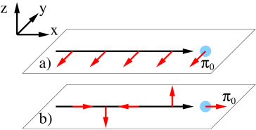
Figure 1: (color online) Demonstration of the spin dynamics of plane waves a) with and b) without definite helicity (Eq. (10)). a) $\gamma=(1,0)$, b) $\gamma=(1,i)/\sqrt{2}$. In both figures, the black arrow denotes the direction of propagation ($\varphi_{\rm i}=0$), the red arrows denote the local polarization vector, and the circle denotes the origin. $\text{\boldmath{$\pi$}}_{0}$ is the polarization vector in the origin.

In order to consider the scattering of the plane waves without definite helicity in (10), we introduce the $2\times 2$ complex matrix

$$D(r,\varphi)=\left(e^{ik_{+}r}\eta_{+}(\varphi),e^{ik_{-}r}\eta_{-}(\varphi)\right).$$ (11)

Note that for every $r$ and $\varphi$, $D$ is unitary. With this notation, the scattered part of the wave function describing the scattering process of the superposed plane wave (10) is

$$\tilde{\psi}^{\rm(sc)}_{\gamma,\varphi_{\rm i}}(r,\varphi)=\sum\limits_{\tau}\tilde{\psi}^{\rm(sc)}_{\tau,\varphi_{\rm i}}(r,\varphi)\gamma_{\tau}=\frac{1}{\sqrt{r}}D(r,\varphi)f(\varphi,\varphi_{\rm i})\gamma$$ (12)

The differential scattering cross section is

$$\sigma_{\rm diff}(\varphi,\varphi_{\rm i};\gamma)=r|\tilde{\psi}^{\rm(sc)}_{\gamma,\varphi_{\rm i}}(r,\varphi)|^{2}.$$ (13)

Since $D$ is unitary, the differential cross section does not depend on $r$, as it is expected:

$$\sigma_{\rm diff}(\varphi,\varphi_{\rm i};\gamma)=\gamma^{\dagger}[f(\varphi,\varphi_{\rm i})]^{\dagger}f(\varphi,\varphi_{\rm i})\gamma.$$ (14)

In order to get a more transparent formula, we take the expansion of the scattering amplitude matrix using the unit matrix $\sigma_{0}$ and the Pauli matrices $\sigma_{1}$, $\sigma_{2}$, $\sigma_{3}$:

$$f(\varphi,\varphi_{\rm i})=\sum\limits_{m=0}^{3}u_{m}(\varphi,\varphi_{\rm i})\sigma_{m}.$$ (15)

The differential scattering cross section in terms of these coefficients $u$ is

$$\sigma_{\rm diff}(\varphi,\varphi_{\rm i};\gamma)=c(\varphi,\varphi_{\rm i})+{\bf v}(\varphi,\varphi_{\rm i})\cdot{\bf P}(\gamma),$$ (16)

with

$$c = \sum\limits_{m=0}^{3}|u_{m}|^{2},$$ (17)

$${\bf v} = 2\ {\rm Re}(u_{0}^{*}{\bf u})-i({\bf u}\times{\bf u}^{*}),$$ (18)

$${\bf P}(\gamma) = \gamma^{\dagger}\mbox{\boldmath{$\sigma$}}\gamma.$$ (19)

Here $\text{\boldmath{$\sigma$}}=(\sigma_{x},\sigma_{y},\sigma_{z})$, therefore ${\bf P}(\gamma)$ is a three-dimensional unit vector for arbitrary $\gamma\in S_{1}(\mathbb{C}^{2})$. In equation (16) the differential scattering cross section corresponding to the angle $\varphi$ is written in terms of the $S$-matrix (hidden in $c$ and ${\bf v}$), the propagation direction of the incoming plane wave $\varphi_{\rm i}$ and the complex vector $\gamma$ characterizing the superposed, non-helicity-eigenstate plane wave. The result (16) is completely general, valid for arbitrary finite-range scattering potentials. This formula will play a central role in the derivation of the main result of our paper.

To substitute the rather formal quantity $\gamma$ with a real physical quantity in (16), we can use the polarization vector of the superposed plane wave in the origin,

$$\text{\boldmath{$\pi$}}_{0}(\gamma,\varphi_{\rm i})={\bf P}\left(\phi_{\gamma,\varphi_{\rm i}}({\bf r}=0)\right)$$ (20)

instead. Note that the ${\bf P}$ function is defined in (19). It can be shown that the following relation holds between the formal quantity ${\bf P}(\gamma)$ and the real physical quantity $\text{\boldmath{$\pi$}}_{0}(\gamma,\varphi_{\rm i})$ :

$$\text{\boldmath{$\pi$}}_{0}(\gamma,\varphi_{\rm i})=\left(\begin{array}[]{ccc}0&\cos\varphi_{\rm i}&\sin\varphi_{\rm i}\\ 0&\sin\varphi_{\rm i}&-\cos\varphi_{\rm i}\\ -1&0&0\end{array}\right)\cdot{\bf P}(\gamma).$$ (21)

This relation can easily be checked for the examples shown in Fig. 1. Equation (16) together with (21) expresses the differential scattering cross section corresponding to the angle $\varphi$ as the function of the plane wave propagation direction $\varphi_{\rm i}$, the $S$-matrix and the polarization vector of the incoming plane wave in the origin $\text{\boldmath{$\pi$}}_{0}$.

III Simple scattering potentials

The derivation so far has been completely general. Now we restrict our analysis to special scattering potentials. We call the $V$ scattering potential simple, if it preserves the three fundamental symmetries of the Rashba Hamiltonian $H_{0}$: time reversal ($i\sigma_{y}C$, where $C$ is the complex conjugation), rotation around the $z$ axis ($J_{z}=-i\hbar\partial_{\varphi}+\hbar\sigma_{z}/2$) and the combined symmetry of real space reflection and spin rotation ($\sigma_{y}P_{x}$, where $P_{x}$ is the spatial reflection with respect to the $x$ axis). It is clear that the spin-independent central potentials are simple.

For simple scattering potentials, the three symmetry operations above are compatible with $H$, which will result in a remarkable simplification of the $S$ matrix and, therefore, of $\sigma_{\rm diff}$. It can be shown that the consequence of the time reversal, rotational and combined symmetries, respectively:

$$S^{(j^{\prime}j)}_{\tau^{\prime}\tau} = \tau^{\prime}\tau e^{i(j-j^{\prime})\pi}S^{(-j,-j^{\prime})}_{\tau\tau^{\prime}},$$ (22)

$$S^{(j^{\prime}j)}_{\tau^{\prime}\tau} = \delta_{j^{\prime}j}S^{(jj)}_{\tau^{\prime}\tau},$$ (23)

$$S^{(j^{\prime}j)}_{\tau^{\prime}\tau} = \tau^{\prime}\tau e^{i(j-j^{\prime})\pi}S^{(-j^{\prime},-j)}_{\tau^{\prime}\tau}.$$ (24)

As a consequence of these relations, the scattering amplitude matrix – and hence every quantity derived from that – depends only on the scattering angle $\theta=\varphi-\varphi_{\rm i}$. The explicit form of $f$ for simple scattering potentials:

$$f_{\tau,\tau}(\theta) = \sqrt{\frac{2}{\pi ik_{\tau}}}\sum\limits_{j\in\mathbb{J}^{+}}\cos(j\theta)F^{(jj)}_{\tau,\tau},$$ (25)

$$f_{-\tau,\tau}(\theta) = \sqrt{\frac{2i}{\pi k_{\tau}}}\sum\limits_{j\in\mathbb{J}^{+}}\sin(j\theta)F^{(jj)}_{-\tau,\tau}.$$ (26)

Note that the diagonal (off-diagonal) elements of the scattering amplitude matrix $f$ are even (odd) functions of the scattering angle $\theta$.

By definition, skew scattering is absent in the process if the differential cross section $\sigma_{\rm diff}$ in (16) is an even function of the scattering angle $\theta$ for every $\gamma\in S_{1}(\mathbb{C}^{2})$. Using the symmetry properties of the components of the scattering amplitude matrix $f$, one can show that $c$ and $v_{3}$ are even functions of $\theta$. On the other hand, $v_{1}$ and $v_{2}$ are odd. It means that the absence of skew scattering is not provided by the symmetry properties of the total Hamiltonian even if the scattering potential is simple. This is the main result of our paper.

To be a bit more specific, we can say that if the incoming plane wave has a definite helicity, i.e. $\gamma\propto(1,0)$ or $\gamma\propto(0,1)$, then using (19) we get ${\bf P}(\gamma)\parallel(0,0,1)$, therefore equation (16) and the even character of $c$ and $v_{3}$ implies the absence of skew scattering. On the other hand, if the incoming plane wave is a finite superposition of the two helicity eigenstates (i.e. both components of $\gamma$ are finite), then the skew scattering effect arises if $v_{1}$ or $v_{2}$ are finite. We note that obviously our symmetry considerations are not capable to tell whether $v_{1}$ or $v_{2}$ is finite or not – having a specific $V$ potential in hand, we have to solve the scattering problem and calculate the elements of the $S$-matrix in order to learn the answer.

IV Hard wall impurity model

In order to demonstrate the predicted skew scattering effect, we present exact results for a hard wall potential:

$$V(r)=\left\{\begin{array}[]{cl}0&\mbox{if }r>R\\ \infty&\mbox{otherwise}\end{array}\right.$$ (27)

This potential $V$ is simple. We refer to Refs.  yeh, and walls, for the derivation of the elements of the $S$ matrix.

We focus on the low-energy properties of the scattering, i.e. $kR\ll 1$, because this limit corresponds to the most widely studied short-range impurity modelsinoue ; mishchenko ; raimondi . If we consider the scattering of electrons at the Fermi energy, then it is realistic to set the parameter $k_{\textrm{so}}/k$ between zero and $0.1$grundler . Exact results for such parameter values are shown in Fig. 2, where we have plotted the angular dependence of the key quantities $c$, $v_{1}$, $v_{2}$ and $v_{3}$ defined in eqs. (17) and (18). Apparently, $v_{1}$ and $v_{2}$ does not vanish for finite $k_{\textrm{so}}$, therefore skew scattering is present in the process indeed. Other features of the results are summarized as: (i) the quantity $c$ is practically independent of $k_{\textrm{so}}$; (ii) for $k_{\textrm{so}}=0$ we have ${\bf v}=0$, therefore the differential cross section (which is equal to $c$ in this case) is spin-independent, symmetric in $\theta$ and approximately a constant function of $\theta$; (iii) for finite $k_{\textrm{so}}$, the magnitude of $v_{1}$ is much smaller than that of $v_{2}$ and $v_{3}$; the latter ones appear to have the same magnitude for a given $k_{\textrm{so}}$, and their magnitude seems to scale linearly with $k_{\textrm{so}}$.

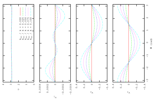
Figure 2: (color online) The quantities $c$, $v_{1}$, $v_{2}$ and $v_{3}$ (in units of $R$) determining the differential scattering cross section (see eq. (16)) as functions of the scattering angle $\theta=\varphi-\varphi_{\rm i}$ for a central hard wall potential. $kR$ = 0.04.

We present the exact differential cross sections calculated using (16) in Fig. 3, corresponding to the two example plane waves of Fig. 1. The $\sigma_{\rm diff}$ of the plane wave with definite helicity (a) is symmetric, but for the superposed plane wave (b) the skew scattering effect is clearly visible even for the realistic value of $k_{\rm so}/k=0.1$.

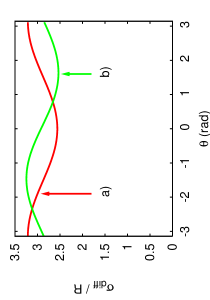
Figure 3: (color online) Differential scattering cross sections exactly calculated in the hard wall impurity model, corresponding to the incoming plane waves of Fig. 1: a) $\gamma=(1,0)$, b) $\gamma=(1,i)/\sqrt{2}$. $kR=0.04$ and $k_{\rm so}/k=0.1$.

In order to understand the features (i) – (iii) of the exact results for the key quantities $c$ and ${\bf v}$ (shown in Fig. 2), we calculate them in the first Born approximation for the simplest potential modeling short-range impurites: $V({\bf r})=\kappa\delta({\bf r})$, where $\delta$ is the Dirac-delta and $\kappa$ represents the strength of the potential. For the incoming plane wave in (10), the scattered wave within this approach ismott ; ballentine

$$\psi^{\rm(sc)}_{\gamma,\varphi_{\rm i}}=G^{+}_{E}V\phi_{\gamma,\varphi_{\rm i}},$$ (28)

where $G^{+}_{E}$ is the retarded Green’s function of the Rashba Hamiltonian $H_{0}$. The exact form of the Green’s function in position representation is known. walls ; rashbabilliard Exploiting the simple form of our potential, we find

$$\psi^{\rm(sc)}_{\gamma,\varphi_{\rm i}}({\bf r})=\kappa G^{+}_{E}({\bf r},0)\phi_{\gamma,\varphi_{\rm i}}(0),$$ (29)

where $G^{+}_{E}({\bf r},{\bf r}^{\prime})$ is the position matrix element of $G^{+}_{E}$. The first step to derive the scattering amplitude matrix is taking the $|{\bf r}|\to\infty$ limit of the actual form of $G^{+}_{E}({\bf r},0)$, and calculating $\tilde{\psi}^{\rm(sc)}_{\gamma,\varphi_{\rm i}}$. After that, one can derive the components of $f$ using (12). With some algebra one gets the following results with respect to $c$ and $\bf v$:

$$c(\theta) = \frac{(m^{*}\kappa)^{2}}{2\pi\hbar^{4}k}=c_{0},$$ (30)

$$v_{1}(\theta) = 0,$$ (31)

$$v_{2}(\theta) = -\sin(\theta)c_{0}\frac{k_{\textrm{so}}}{k},$$ (32)

$$v_{3}(\theta) = -\cos(\theta)c_{0}\frac{k_{\textrm{so}}}{k}$$ (33)

The qualitative similarity between these results and the exact ones in Fig 2 is remarkable. Apparently, the results of this simple short-range impurity model grasp all the features (i), (ii) and (iii) of the exact results for $kR\ll 1$ listed before. For $k_{\textrm{so}}=0$ we recover the isotropic, spin-independent differential scattering cross section $\sigma_{\rm diff}(\theta)=c_{0}$, as it is expected. Including only one further parameter $k_{\textrm{so}}/k$, our results (30-33) provide a generalization of the one-parameter isotropic model for scattering in the presence of Rashba SOI.

V Summary

The knowledge of the properties of electron scattering can be the starting point for further theoretical predictions of impurity-related solid state phenomena. The theory of effects related to single, isolated impurities, like the Friedel oscillation, Landauer’s charge dipoledittrich and the spin cloud predicted by Mal’shukov and Chumalshukov can be based on the knowledge of the scattering amplitude matrix $f$. In Boltzmann transport theory, the transition probabilities are needed as an input information in the evaluation of the collision integralashcroft . Hence the exact formalism presented in this paper can serve as a firm foundation of further theoretical investigations. The two-parameter model for short-range impurities provides a convenient tool to replace the isotropic approximation in systems with significant Rashba SOI.

In conclusion, we have generalized the formalism of two-dimensional elastic quantum scattering to systems with finite Rashba spin-orbit coupling. Based on symmetry considerations, we have shown that the differential scattering cross section becomes spin-dependent and can show the skew scattering effect even if the scattering potential is central and spin-independent. We have demonstrated the skew scattering by exact results of the hard wall impurity model. We derived the differential cross section in the first Born approximation for a Dirac delta scattering potential, and found remarkable similarity between these approximation and the exact results for low scattering energies. Using the simple formulas gained from the Born approximation, we proposed a two parameter model to substitute the isotropic or $s$-wave model of short-range impurity scattering in the presence of Rashba coupling.

We acknowledge fruitful discussions with Cs. Péterfalvi. This work is supported by European Commission Contract No. MRTN-CT-2003-504574.

References

- (1) N. F. Mott and H. S. Massey, The Theory of Atomic Collisions, (3rd ed. Oxford University Press, Oxford, 1965).
- (2) L. E. Ballentine, Quantum Mechanics: A Modern Development, (World Scientific, Singapore, 1998).
- (3) J. Smit, Physica 21, 877 (1955).
- (4) J. Smit, Physica 24, 39 (1958).
- (5) A. Crépieux, P. Bruno, Phys. Rev. B 64, 014416 (2001).
- (6) J. E. Hirsch, Phys. Rev. Lett. 83, 1834 (1999).
- (7) H.-A. Engel, B. I. Halperin, E. I. Rashba, Phys. Rev. Lett. 95, 166605 (2005).
- (8) Y. K. Kato, R. C. Myers, A. C. Gossard, D. D. Awschalom, Science 306, 1910 (2004).
- (9) H.-A. Engel, E. I. Rashba, B. I. Halperin, cond-mat/0603306 (unpublished).
- (10) R. Winkler, Spin-Orbit Coupling Effects in Two-Dimensional Electron and Hole Systems (Springer, Berlin, 2003).
- (11) G. Dresselhaus, Phys. Rev. 100, 580 (1955).
- (12) E. I. Rashba, Fiz. Tverd. Tela Leningrad 2, 1224 (1960) [Sov. Phys. Solid State 2, 1109 (1960)]; Yu. A. Bychkov, E. I. Rashba, J. Phys. C 17, 6039 (1984).
- (13) A. G. Mal’shukov, C. S. Chu, Phys. Rev. Lett. 97, 076601 (2006).
- (14) A. V. Shytov, E. G. Mishchenko, H.-A. Engel, B. I. Halperin, Phys. Rev. B 73, 075316 (2006);
- (15) H.-A. Engel, E. I. Rashba, B. I. Halperin, Phys. Rev. Lett. 98, 036602 (2007).
- (16) J. I. Inoue, G. E. W. Bauer, and L. W. Molenkamp, Phys. Rev. B 70, 041303(R) (2004).
- (17) E. G. Mishchenko, A. V. Shytov, and B. I. Halperin, Phys. Rev. Lett. 93, 226602 (2004).
- (18) R. Raimondi, P. Schwab, Phys. Rev. B 71, 033311 (2005).
- (19) Jr-Yu Yeh, M.-Che Chang, and C.-Yu Mou, Phys. Rev. B 73, 035313 (2006) .
- (20) J. D. Walls, J. Huang, R. M. Westervelt, and E. J. Heller, Phys. Rev. B 73, 035325 (2006).
- (21) Strictly speaking, the term ‘-wave scattering’ is paradoxical in the context of the Rashba Hamiltonian: would refer to partial waves with zero orbital angular momentum, however, orbital angular momentum is not a good quantum number if the Rashba strength is finite.
- (22) J. Cserti, A. Csordás and U. Zülicke, Phys. Rev. B 70, 233307 (2004); A. Csordás, J. Cserti, A. Pályi, U. Zülicke, Eur. Phys. J. B 54, 189 (2006).
- (23) Handbook of Mathematical Functions, edited by M. Abramowitz and I. A. Stegun (Dover, New York, 1972).
- (24) S. Datta and B. Das, Appl. Phys. Lett. 56, 665 (1990).
- (25) D. Grundler, Phys. Rev. Lett. 84, 6074 (2000).
- (26) T. Dittrich et al., Quantum Transport and Dissipation (Wiley-VCH, Weinheim, 1998).
- (27) N. W. Ashcroft, N. D. Mermin, Solid State Physics (Saunders College Publishing, Philadelphia, 1976).