Nonequilibrium charge dynamics of light-driven rings threaded by a magnetic flux

Abstract

We study theoretically the charge polarization and the charge current dynamics of a mesoscopic ring driven by short asymmetric electromagnetic pulses and threaded by an external static magnetic flux. It is shown that the pulse-induced charge polarization and the associated light-emission is controllable by tuning the external magnetic flux. Applying two mutually perpendicular pulses triggers a charge current in the ring. The interplay between this nonequilibrium and the persistent currents is investigated and the conditions under which the pulses stop the persistent current are identified.

1 INTRODUCTION

Quantum structures with a ring confining geometry have served over the years as a paradigm for the demonstration of quantum-interference phenomena such as the Aharonov-Bohm effect and the persistent (equilibrium) current [1, 2, 3, 4] that emerges if the ring is pierced by a static magnetic flux. The persistent current has also been considered when a time-dependent magnetic field with a static component [5, 6, 7, 8, 9, 10, 11, 12] being applied, and it has been found that the current diminishes when the static component vanishes. Another possibility for generating (nonequilibrium) current is to irradiate the ring with circular polarized light, [13, 14, 15] and references therein. In principle, this approach is feasible for a size-quantized system and if the radiation frequency is tuned such that the rotating-wave approximation is applicable and counter-rotating contributions to the current are thus negligible. Hence, this approach is expected to be particularly useful for molecular ring structure, cf. ref. [15] and references therein. Another approach for current generation which does not rely on the level quantization and resonant excitations, is based on an asymmetry of the electric field amplitude of the applied pulse [16, 17]. As experimentally demonstrated [18, 19, 20, 21] the optical cycle of such asymmetric pulses consists of a short and strong half cycle followed by a much longer and weak half cycle of an opposite polarity. The charge dynamics is mainly triggered by the strong , short half cycle [16, 17, 23, 22] and hence these pulses are referred to as half-cycle pulses (HCP). In general, HCPs are capable of inducing nonequilibrium electric dipole and direct charge currents [17, 23, 22], even if the system is not lacking an inversion symmetry, in contrast to the well-known photovoltaic effect [24, 25]. For isolated rings (and without an external magnetic flux), applying one linearly polarized HCP induces a charge polarization. Applying in a perpendicular direction to the first pulse a second HCP leads to a charge current that can be tuned by varying the properties and the time-delay between the two pulses. The question which has not yet been addressed and will be of concern here is how the HCPs-induced charge polarization and the charge current are influenced by the persistent current generated by a static magnetic flux. As shown below, the HCP-induced nonequilibrium charge polarization and the associated emitted radiation are tunable by changing the magnitude of the static magnetic flux. The nonequilibrium current triggered by two time-delayed HCPs can be tuned to cancel the magnetic-flux-induced equilibrium current offering thus a possibility for time switching of the persistent current on a picosecond time-scale.

2 Theoretical model

For the sake of simplicity, we consider here an isolated single channel 1D ballistic ring with $N$ electrons and radius $\rho_{0}$ at low temperatures. This treatment is appropriate if the width and the height of the ring are smaller than both the ring radius and the Fermi wavelength of the carriers. The generalization to the multi-channel case can be done along the lines of Refs.[16, 26] where it is shown that the multi-channel case does not change qualitatively the predictions of the 1D model. The ring is pierced by an external magnetic flux $\phi$ and is subjected to a sequence of short, linearly polarized half-cycle pulses. The light propagation direction is perpendicular to the plane of the ring. The Hamiltonian describing the dynamics of the system is given by

$$\hat{H}(t)=\hat{H}_{0}+\hat{V}_{int},$$ (1)

where

$$\hat{H}_{0}=\frac{1}{2m^{\ast}\rho_{0}^{2}}\left(-i\hbar\frac{\partial}{\partial\theta}+\hbar\frac{\phi}{\phi_{0}}\right)^{2}\;\;;\;\;\hat{V}_{int}=e\mathbf{E}(t)\cdot\mbox{\boldmath$\rho$}.$$ (2)

Here $e$ is the elementary charge, $\mathbf{E}(t)$ stands for the time-dependent electric field of the applied pulses and the vector $\mbox{\boldmath$\rho$}=(\rho_{0}\cos\theta,\rho_{0}\sin\theta)$ describes the electron position. $m^{\ast}$ and $\phi_{0}$ are the electron effective mass and the flux quantum, respectively. In what follows we expand the field operator $\hat{\Psi}(\theta,t)$ on a basis of eigenstates $\varphi_{n}(\theta)$ of $\hat{H}_{0}$, i.e.,

$$\hat{\Psi}(\theta,t)=\sum_{n}\hat{c}_{n}(t)\varphi_{n}(\theta),\quad\hat{H}_{0}\varphi_{n}(\theta)=E_{n}^{(0)}\varphi_{n}(\theta).$$ (3)

The components of the time-dependent density matrix are expressed as $\rho_{mn}(t)=\langle\hat{c}_{m}^{{\dagger}}(t)\hat{c}_{n}(t)\rangle$. Here $\langle...\rangle$ denotes the expectation value which is taken with respect to the initial state of the system.

Now we turn to the specification of the employed light pulses. The duration $\tau_{d}$ of the experimentally available HCPs is in the subpicosecond time scale. On the other hand, for typical ballistic mesoscopic rings ($\rho_{0}\sim 1\mu m$) the time $\tau_{{}_{F}}$ a particle at the Fermi level needs for a round trip is tens of picoseconds, meaning that $\tau_{d}\ll\tau_{{}_{F}}$. In this case, the so-called impulsive approximation (IA) can be employed to describe accurately the dynamics of the system [27]. Within the IA the action of the HCPs is encompassed in the matching conditions (4) for the density matrix at the instances before and after the pulses are applied while the system propagates in a pulse-free manner at any other time[28] (note that in absence of the pulses the magnetic flux is still present). To be specific, let us consider the case where two HCPs that are linearly polarized in the $x$ and $y$ directions are applied respectively at the times $t_{1}=0$ and $t_{2}=\tau$. For the density matrix we find within the IA that (we use the abbreviation $|\varphi_{n}(\theta)\rangle\equiv|n\rangle$)

$$\begin{split}&\rho_{mn}(0^{+})=\sum_{k,l}\langle n|e^{-i\alpha_{1}\cos\theta}|l\rangle\langle k|e^{i\alpha_{1}\cos\theta}|m\rangle\rho_{kl}(0^{-});\\ &\rho_{mn}(\tau^{+})=\sum_{k,l}\langle n|e^{-i\alpha_{2}\sin\theta}|l\rangle\langle k|e^{i\alpha_{2}\sin\theta}|m\rangle\rho_{kl}(\tau^{-}).\end{split}$$ (4)

Here the dimensionless quantity $\alpha_{j}$ characterizes the action transferred to the system

$$\alpha_{j}=\rho_{0}p_{j}/\hbar,$$ (5)

while $p_{j}$ describes the strength of the pulse $E_{j}$

$$p_{j}=e\int_{t_{j}}^{t_{j}+\tau_{d}}E_{j}(t)dt.$$ (6)

The subindex $j=1,2$ refers to the first and second pulse (with the same duration $\tau_{d}$). We remark here that for a different propagation direction of HCPs, e.g. in the plane of the ring, and/or for the strong excitation regime ($\alpha\gg 1$) the time-dependent magnetic-field component of the pulse may in general affect the dynamics of the electron system and should be included in the Hamiltonian (1). This is to be contrasted with the case discussed in this paper where the magnetic field associated with the HCP is moderate and lies in the plane of the ring (where electrons are confined).

Within the relaxation time approximation the equation of motion for the density matrix reads

$$\begin{split}\frac{\partial\rho_{mn}}{\partial t}=&i\frac{E_{m}^{(0)}-E_{n}^{(0)}}{\hbar}\rho_{mn}\\ &-\frac{\delta_{mn}}{T_{1}}\left[\rho_{mn}-\rho_{nn}(0^{-})\right]-\frac{1-\delta_{mn}}{T_{2}}\rho_{mn},\end{split}$$ (7)

where $\delta_{mn}$ is the Kronecker symbol and $T_{1}$ and $T_{2}$ are the relaxation and dephasing times, respectively. Eqs.(4)-(7) together with the initial condition that before the application of the pulses the system is in a thermal equilibrium, i.e.,

$$\rho_{mn}(0^{-})=2\delta_{mn}\left(1+e^{-\frac{[E_{n}^{(0)}-\eta]}{k_{{}_{B}}T}}\right)^{-1},$$ (8)

determine completely the time evolution of the density matrix. The factor 2 in the Fermi-Dirac distribution (8) accounts for the two-fold spin degeneracy and the chemical potential $\eta$ is set by the requirement of the conservation of the particles’ number $N$.

We are particularly interested in the study of the charge polarization and the currents induced in the ring. The charge polarization along the $x$ axis is determined by the $x$-component of the dipole moment operator. After some algebra one obtains for the charge polarization

$$\mu(t)=-e\rho_{0}\textrm{Re}\left[\sum_{n}\rho_{n,n-1}(t)\right].$$ (9)

This result is remarkable. It tells us that the time dependence of the charge polarization does not depend on the time evolution of the diagonal components of the density matrix, i.e., by tracing the evolution of the induced polarization one can obtain physical information that is exclusively due to dephasing.

Using the first of eqs. (4) and eqs. (7)-(9) and performing the same steps as in ref. [22] we can write the charge polarization of the ring after the application of the first HCP as

$$\begin{split}\mu(t)=-&e\rho_{0}\alpha_{1}\Theta(t)[J_{0}(\Omega)+J_{2}(\Omega)]\sin\!\!\left[\frac{2\pi t}{t_{p}}\right]e^{-t/T_{2}}\\ &\times\sum_{n}\rho_{nn}(0^{-})\cos\!\!\left[\frac{4\pi t}{t_{p}}\left(n+\frac{\phi}{\phi_{0}}\right)\right],\end{split}$$ (10)

where $\Theta(x)$ denotes the Heaviside step function and $J_{l}(x)$ is a Bessel function of the order $l$. Furthermore, we introduced the quantities

$$\Omega=\alpha_{1}\sqrt{2-2\cos(4\pi t/t_{p})},$$ (11)

$$t_{p}=4\pi m^{\ast}\rho_{0}^{2}/\hbar.$$ (12)

The charge current density operator can be expressed in terms of the field operators (3) and the angular component of the vector potential $A_{\theta}=\phi/(2\pi\rho_{0})$ as follows

$$\begin{split}\hat{j}=&\frac{ie\hbar}{2m^{\ast}\rho_{0}^{2}}\left[\hat{\Psi}^{{\dagger}}(\theta,t)\frac{\partial\hat{\Psi}(\theta,t)}{\partial\theta}-\frac{\partial\hat{\Psi}^{{\dagger}}(\theta,t)}{\partial\theta}\hat{\Psi}(\theta,t)\right]\\ &-\frac{e^{2}}{\rho_{0}m^{\ast}c}\hat{\Psi}^{{\dagger}}(\theta,t)A_{\theta}\hat{\Psi}(\theta,t).\end{split}$$ (13)

Upon mathematical manipulations we find for the charge current

$$I(t)=\langle\langle\hat{j}\rangle\rangle=I_{0}\sum_{n}(n+\phi/\phi_{0})\rho_{nn}(t).$$ (14)

Here

$$I_{0}=-e\hbar/(m^{\ast}\rho_{0}^{2})$$ (15)

sets the scale of the current magnitude. The double bracket $\langle\langle\ldots\rangle\rangle$ stands for angular integration and expectation value computation. In contrast to the charge polarization, the charge current depends only on the diagonal elements of the density matrix. Therefore, dephasing and relaxation can be independently investigated by tracing the charge polarization and the charge current, respectively.

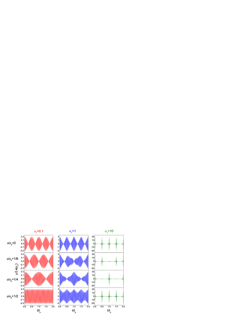
Figure 1: The time dependence of the charge polarization $\mu(t)$ as a function of the magnetic flux $\phi$ for various values of the pulse strengths that result in different values of the transferred action $\alpha_{1}$ (cf.Eq.(5)). For the sin-square HCP having duration $\tau_{d}=1$ ps and the ring radius of $r_{0}=1~{}\mu$m the value of the transferred action $\alpha_{1}=0.1$ ($\alpha_{1}=1$, $\alpha=10$) corresponds to the peak electric field strength $E_{0}=1.32~{}$V/cm ($E_{0}=13.2~{}$V/cm, $E_{0}=132~{}$V/cm). The time is expressed in units of $t_{p}=4\pi m^{\ast}\rho_{0}^{2}/\hbar$.

Exploiting Eqs. (4)-(7) and (14) we deduce after some algebra the following relation for the total charge current

$$I(t)=I_{pers}+\Theta(t-\tau)I_{dyn}(t),$$ (16)

where

$$I_{pers}=I_{0}\sum_{n}(n+\phi/\phi_{0})\rho_{nn}(0^{-})$$ (17)

is a static (persistent current) component induced by the magnetic flux and

$$I_{dyn}(t)=\frac{I_{0}\alpha_{2}}{e\rho_{0}}\mu(\tau)e^{-t/T_{1}}$$ (18)

is a dynamical component due to the action of the pulses and is determined by the polarization $\mu(\tau)$ of the ring at the time the second pulse is applied [16]. Note also that the dynamical component of the current only appears after the second pulse is applied, i.e., it is necessary to apply two orthogonal linearly polarized HCPs in order to produce an additional clock-wise anti-clock-wise symmetry breaking [16] (in case of the persistent current this symmetry break is brought about by the magnetic-flux induced time-reversal symmetry breaking).

It follows from eq. (16) that the static part of the total charge current induced in the ring does not depend on the application of the HCPs and is not modified by them (i.e., the persistent current is really persistent). On the other hand, the dynamical component $I_{dyn}$ depends on both the external magnetic flux and the pulse parameters because, as shown below explicitly, the dipole moment $\mu(\tau)$ is a function of $\phi$.

An important consequence of eqs. (16) and (18) is that a magnetic-flux induced persistent current in a ballistic ring can be temporally stopped by applying HCPs, for all the parameters determining the sign and the magnitude of $I_{dyn}$ are known [cf. eqs. (5), (15) and (19)]. We note that the build-up time of $I_{dyn}$ (which determines the switch-off time of $I$, i.e. the cancellation of $I_{pers}$) is set by the duration of the HCP which can be in the subpicosecond regime. As $I_{dyn}$ relaxes according to eq. (18) $I_{pers}$ emerges again, however, upon the application of another sequence of HCPs we can switch off again the total current (16).

It should be remarked here that the decomposition of the charge current in a statical and a dynamical component is valid within the relaxation time approximation employed here. It might well be that the inclusion of memory and non-linear effects prevents such a simple structure of the current. A definitive conclusion on this point would require the treatment of two-particle and higher order correlations that is a challenging task for inhomogeneous distributions (non-diagonal density matrix elements). On the other hand, for weak excitations and small temperatures we expect nonlinear effects (in the field strength and in relaxation) to be marginal and the correlation effects on the relaxation to be of less importance (due to the same reasons as for the ground state).

3 Explicit results and numerical demonstrations

For zero temperature we were able to perform the sum in the eq. (10) analytically to obtain

$$\mu(t)=-e\rho_{0}\alpha_{1}\Theta(t)[J_{0}(\Omega)+J_{2}(\Omega)]s(t)e^{-t/T_{2}},$$ (19)

where

$$\begin{split}s(t)\!=&2\cos\!\left[\frac{4\pi t}{t_{p}}\left(\left|\frac{\phi}{\phi_{0}}\right|\!-\!\frac{1}{2}\right)\right]\sin\!\left[\frac{N\pi t}{t_{p}}\right],\hskip 5.69046ptN\!=0\ ({\rm mod}\;4);\\ s(t)\!=&\cos\!\left[\frac{4\pi t}{t_{p}}\frac{\phi}{\phi_{0}}\right]\!\sin\!\left[\frac{(N+1)\pi t}{t_{p}}\right]\\ &+\cos\!\left[\frac{4\pi t}{t_{p}}\left(\left|\frac{\phi}{\phi_{0}}\right|\!-\!\frac{1}{2}\right)\right]\!\sin\!\left[\frac{(N-1)\pi t}{t_{p}}\right],\\ &\hskip 156.49014ptN\!=1\ ({\rm mod}\;4);\\ s(t)\!=&2\cos\!\left[\frac{4\pi t}{t_{p}}\frac{\phi}{\phi_{0}}\right]\sin\!\left[\frac{N\pi t}{t_{p}}\right],\hskip 44.10185ptN\!=2\ ({\rm mod}\;4);\\ s(t)\!=&\cos\!\left[\frac{4\pi t}{t_{p}}\left(\left|\frac{\phi}{\phi_{0}}\right|\!-\!\frac{1}{2}\right)\right]\!\sin\!\left[\frac{(N+1)\pi t}{t_{p}}\right]\\ &+\cos\!\left[\frac{4\pi t}{t_{p}}\frac{\phi}{\phi_{0}}\right]\!\sin\!\left[\frac{(N-1)\pi t}{t_{p}}\right],\hskip 15.6491ptN\!=3\ ({\rm mod}\;4).\end{split}$$ (20)

These results apply for $\phi/\phi_{0}\in[-1/2,1/2]$, otherwise $s(t;\phi/\phi_{0})$ is given by the periodicity condition $s(t;\phi/\phi_{0}+1)$=$s(t;\phi/\phi_{0})$. In the limiting case $\phi=0$ eqs. (20) simplify to the results obtained in ref. [22]. Inserting the expressions for $\mu(t)$ given by eqs. (19) and (20) at $t=\tau$ into eq. (18) yields an analytical expression for the dynamical part of the current. The persistent part of the current was calculated previously in ref. [29].

For an illustration we performed explicit calculations for the case of a 1D GaAs ring with $N=100$, radius $\rho_{0}=1\;\mu\textrm{m}$ at zero temperature. The time dependence (ignoring the effects of dephasing [30]) of the induced charge polarization is shown in fig. 1 for different values of the external magnetic flux $\phi$ and pulse strengths yielding different $\alpha_{1}$ [cf. eq. (5)]. The time is expressed in units of the characteristic time $t_{p}$. For certainty we assume here that the time profile of the HCP electric field is given by $E(t)=E_{0}\sin^{2}[\pi t/\tau_{d}]$ for $t\in(0,\tau_{d})$ and $E(t)=0$ outside of this time interval. In this case we have $\alpha_{1}=\rho_{0}eE_{0}\tau_{d}/(2\hbar)$. As seen from fig. 1 different patterns of the charge polarization evolution can be tailored by changing the applied flux and/or the pulse strength. This observation is of particular relevance since the emission properties of the ring are determined by the time oscillations of the charge polarization [17, 31]. Thus, the system proposed here could serve as a source of electromagnetic radiation with magnetic-flux controllable properties. Another remarkable fact revealed by fig. 1 is the presence of beating behaviour of the charge polarization dynamics in the low excitation regime as well as collapses and revivals of the polarization at higher excitations signifying the important role of quantum interferences [17].

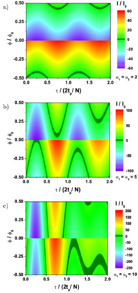
Figure 2: Dependence of the peak current $I$ on the magnetic flux $\phi$ and the time delay $\tau$ between the pulses for different values of the pulse strengths: a) $\alpha_{1}=\alpha_{2}=2$, b) $\alpha_{1}=\alpha_{2}=5$ and c) $\alpha_{1}=\alpha_{2}=10$.

Now we consider the current dynamics. As an example, fig. 2 shows the dependence of the peak current on the magnetic flux and the time delay between the two pulses that trigger $I_{dyn}$. The peak current is given in units of $I_{0}$ (e.g., for a ring with $\rho_{0}=1\;\mu\textrm{m}$ and $N=100$ we have $I_{0}=3\textrm{ nA}$). The total charge current has an oscillatory behavior when scanning $\phi$ and $\tau$. In particular, both the magnitude and the sign of the peak current can be changed by appropriately varying $\phi$ and $\tau$. As we outlined above, there exist regions in which the total induced current vanishes due cancellation of the persistent and the dynamical components of the current. As it is seen from the figure the region where the total current is switched off is controllable by sweeping $\phi$, $\tau$ and/or the pulse strengths. All of these parameters are externally tunable and experimentally feasible with current technology.

Strictly speaking, the derived analytical formulas, (16)-(18) and ((19-20)), are only justified for the weak excitation regime. In the strong excitation regime the nonlinear terms in relaxation can couple diagonal and non-diagonal components of the density matrix, and in this way the dynamics of the polarization and current. However, if the relaxation is slow (and we can expect it to be so for low temperatures) it hardly affects the results presented in the numerical illustrations also for the strong excitation regime ($\alpha=5,10$).

Finally we note that the circulating current results in an induced (orbital) magnetization ($M(t)\approx\pi\rho_{0}^{2}I(t)$). The current temporal controllability is reflected in a picosecond switching of the ring magnetization. The above finding can be generalized, particularly in view of potential applications, to the case of trains of HCPs pulses and/or arrays of mesoscopic rings [17, 16]. The first case may serve as a sophisticated source of ultrashort magnetic pulses while the second allows the design of artificially microstructured materials with magnetic properties locally controllable. In view of applying the present scheme to nano and molecular rings [15] we note that this regime is accessed by changing appropriately the parameters of HCPs: The applicability of the above theory is based on the assumption $\tau_{d}\ll t_{p}$ which implies the use of femtosecond HCP for nano-size rings. Such pulses and even attosecond HCPs are currently under discussions [32].

4 Conclusions

In summary, we showed that the time-dependent charge polarization and charge currents can be generated in mesoscopic rings threaded by a magnetic flux and subjected to a sequence of asymmetric electromagnetic pulses. The time dependence of the induced polarization shows different patterns that can be controlled by appropriately adjusting the magnetic flux and the pulse parameters. Quantum interferences result in beatings and revivals of the charge polarization dynamics. The total charge current induced in the ring can be decomposed into a static and a dynamical components. The static component is associated with the persistent current and does not depend on the parameters of the pulses. The dynamical component is expressible analytically and can be tuned to cancel the persistent current allowing thus a picosecond switching of the total current in the ring.

References

- [1] \NameBüttiker M., Imry Y. Landauer R. \REVIEWPhys. Lett. A961983365.
- [2] \NameCheung H.-F., Gefen Y. Riedel E. K. \REVIEWIBM J. Res. Dev.321988359.
- [3] \NameMailly D., Chapelier C. Benoit A. \REVIEWPhys. Rev. Lett.7019932020.
- [4] \NameRabaud W., Samianadayar L., Mailly D., Hasselbach K., Benoît A. Etienne B. \REVIEWPhys. Rev. Lett.8620013124.
- [5] \NameBüttiker M., Imry Y. Landauer R. \REVIEWPhys. Lett. A961983365.
- [6] \NameLévy L. P., Dolan G., Dunsmuir J. Bouchiat H. \REVIEWPhys. Rev. Lett.6419902074.
- [7] \NameChandrasekhar V. et al. \REVIEWPhys. Rev. Lett.6719913578.
- [8] \NameMailly D., Chapelier C. Benoit A. \REVIEWPhys. Rev. Lett.7019932020.
- [9] \NameEfetov K. B. \REVIEWPhys. Rev. Lett.6619912794.
- [10] \NameKravtsov V. E. Yudson V. I. \REVIEWPhys. Rev. Lett.701993210; \NameChalaev O. L. Kravtsov V. E. \REVIEWibid892002176601.
- [11] \NameKopietz P. Völker A. \REVIEWEur. Phys. J. B31998397.
- [12] \NameMoskalets M. Büttiker M. \REVIEWPhys. Rev. B662002245321.
- [13] \NameMagarill L. I. Chaplik A. V. \REVIEWJETP Lett.701999615.
- [14] \NamePershin Y. V. Piermarocchi C. \REVIEWPhys. Rev. B722005245331.
- [15] \NameBarth I., Manz J., Shigeta Y. Yagi K. \REVIEWJ. Am. Chem. Soc.12820067043.
- [16] \NameMatos-Abiague A. Berakdar J. \REVIEWPhys. Rev. Lett.942005166801.
- [17] \NameMoskalenko A. S., Matos-Abiague A. Berakdar J. \REVIEWPhys. Rev. B742006161303.
- [18] \NameYou D., Jones R. R., Bucksbaum P. H. Dykaar D. R. \REVIEWOpt. Lett.181993290.
- [19] \NameBensky T. J., Haeffler G. Jones R. R. \REVIEWPhys. Rev. Lett.7919972018.
- [20] \NameWetzels A., Gürtel A., H. G. Muller L. D. Noordam \REVIEWEur. Phys. J. D142001157.
- [21] \NameFrey M. T. et al. \REVIEWPhys. Rev. A5919991434.
- [22] \NameMatos-Abiague A. Berakdar J. \REVIEWPhys. Rev. B702004195338.
- [23] \NameMoskalenko A. S., Matos-Abiague A. Berakdar J. \REVIEWPhysics Letters A356 2006255-261.
- [24] \NameBelinicher V. I. Sturman B. I. \REVIEWUsp. Fiz. Nauk1301980130 [\REVIEWSov. Phys. Usp.231980199].
- [25] \NameFal’ko V. I. Khmel’nitskii D. E. \REVIEWZh. Eksp. Teor. Fiz.951989186 [\REVIEWSov. Phys. JETP681989186]; \NameFal’ko V. I. \REVIEWEurophys. Lett.81989785.
- [26] \NameMatos-Abiague A. Berakdar J. \REVIEWEurophys. Lett.692005277-283.
- [27] \NameHenriksen N. E. \REVIEWChem. Phys. Lett.3121999196.
- [28] Note that we consider time delays between consecutive pulses that are much shorter than the relaxation and dephasing times. Relaxation and dephasing during the time interval is then neglected.
- [29] \NameLoss D. Goldbart P. \REVIEWPhys. Rev. B43199113762.
- [30] Within the relaxation time approximation, the effect of dephasing consists in an exponential decay of the polarization on a time scale of the order of . For the system considered here is several tens of nanoseconds [17].
- [31] \NameMatos-Abiague A. Berakdar J. \REVIEWPhys. Lett. A3302004113.
- [32] \NamePersson E., Schiessl K., Scrinzi A. Burgdorfer J. \REVIEWPhys. Rev. A742006013818.