Signatures of retroreflection and induced triplet electron-hole correlations in ferromagnet/$s$-wave superconductor structures

Abstract

We present a theoretical study of a ferromagnet/$s$-wave superconductor junction to investigate the signatures of induced triplet correlations in the system. We apply the extended BTK-formalism and allow for an arbitrary magnetization strength/direction of the ferromagnet, a spin-active barrier, Fermi-vector mismatch, and different effective masses in the two systems. It is found that the phase associated with the $xy$-components of the magnetization in the ferromagnet couples with the superconducting phase and induces spin-triplet pairing correlations in the superconductor, if the tunneling barrier acts as a spin-filter. This feature leads to an induced spin-triplet pairing correlation in the ferromagnet, along with a spin-triplet electron-hole coherence due to an interplay between the ferromagnetic and superconducting phase. As our main result, we investigate the experimental signatures of retrorelection, manifested in the tunneling conductance of a ferromagnet/$s$-wave superconductor junction with a spin-active interface.

I Introduction

The proximity effect buzdinRMP in a normal/superconductor (N/S) junction refers to the induced superconducting correlations between electrons and holes in the normal part of the system. Even far away from the junction (typically distances much larger than the superconducting coherence length $\xi$) where the pairing potential is identically equal to zero, these correlations may persist. Consequently, the proximity effect is responsible for a plethora of interesting physical phenomena, including the Josephson effect in S/N/S junctions kulik , the spin-valve effect in ferromagnet/superconductor (F/S) layers buzdin1999 , and the realization of so-called $\pi$-junctions, which in particular have received much attention both theoretically pitheoretical and experimentally piexperimental during the past decades. The understanding of Andreev-reflection processes andreev1964 is crucial when dealing with the proximity effect in N/S systems. Roughly speaking, this phenomenon may be thought of as a a coherently propagating electron with energy less than the superconducting gap $\Delta$ incident from the N side of the barrier being reflected as a coherently propagating hole, while in the process generating a propagating Cooper pair in the S. Such processes are highly relevant in the context of transport properties of N/S heterostructures in the low-energy regime, and have proved to be an effective tool in probing the pairing symmetry of unconventional SCs (see Ref. deutscherRMP, and references therein).
In recent years, the fabrication of ferromagnet/superconductor heterostructures has been subject to substantial advances due to the development of techniques in material growth and high quality interfaces weider ; wei . With an increasing number of recently discovered unconventional superconductors with exotic pairing symmetries saxena ; bauer ; akasawa , there exists an urgent need to refine the traditional methods, such as tunneling spectroscopy, in order to correctly identify the experimental signatures which reveal the nature of the pairing potential for such superconductors. For one thing, this amounts to taking into account effects which are known to be present in tunneling junction experiments and that may significantly influence the conductance spectra, such as local spin-flip processes and the non-ideality of the interface kreuzer . Also, with the aim of producing theoretical tools that may serve as a guide for identifying the superconducting pairing symmetry, possible spin-filter effects of interface in ferromagnet/superconductor heterostructures warrant attention garcia .
Studies of quantum transport in F/S junctions have a long tradition for both conventional and unconventional pairing symmetries in the superconductor jong ; zhu ; zutic99 ; kashiwaya1999 . Currently, such systems have become the subject of much investigation, not only due to their interesting properties from a fundamental physics point of view, but also because such heterostructures may hold great potential for applications in nanotechnological devices. An important characteristic of most F/S junction is that, unlike N/S junctions, retro-reflection is absent for the hole in the F part of the system. This means that the reflected hole, which carries opposite spin of the original electron, does not retrace the trajectory of the incoming electron. The absence of retro-reflection is due to the presence of an exchange interaction. Previous studies of such systems have primarily focused on a magnetization lying in the plane of the F/S junction, where in most cases the barrier contains a pure non-magnetic scattering potential jong ; zhu ; zutic99 . Kashiwaya et al.  kashiwaya1999 included the effect of a magnetic scattering potential in this type of junction, i.e. spin-active barriers, and very recently, it was suggested by Kastening et al.  kastening that the presence of both intrinsic and spin-active scattering potentials in the barrier of a S/S junction may lead to qualitatively new effects for the Josephson current. So far, the influence of the F phase associated with the planar magnetization perpendicular to the interface has been largely unexplored, although Ref. kastening, considers the 1D case of this situation.
It is therefore the purpose of this paper to investigate two interesting features that arise in a F/S junction in the presence of planar magnetization components: i) the interplay between the planar magnetization and the presence of a spin-active barrier may restore retro-reflection for a given parameter range, and ii) the resulting induced electron-hole pair correlations exhibit a coupling between $\phi$ and the S phase $\gamma$. Since our findings suggest that the traditional picture of absent retro-reflection does not hold for planar magnetization with respect to the junction in the presence of a spin-active barrier, we argue that these results are of major importance in the study of F/S junctions. The presence of retro-reflection in a F/S junction thus influences the spin-charge dynamics in a significant way, giving rise to new possibilites of quantum transport involving charge- and spinflow in such a heterostructure. Elucidating the consequences of this is of fundamental importance. It is also of considerable importance in device fabrication, since our results imply that the spin-active properties of a tunneling barrier play a crucial role.

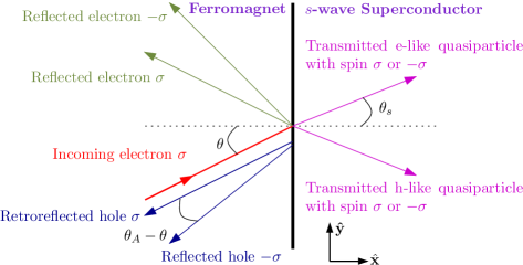
Figure 1: (Color online). Schematic overview of the relevant scattering processes that take place at the F/S interface. We take into account the possibility of retroreflected holes with equal spin as the incoming electron. This is due to the presence of spin-flip processes manifested in the form of planar magnetization and a spin-active barrier.

This paper is organized as follows. In Section II, we define the model we study and set up definitions of the scattering amplitudes to be considered. In Section III we investigate what conditions are necessary for retroreflection to occur. In Section IV, we give our results for the conductance. In Section IV A, we consider the influence of Fermi-vector mismatch on the conductance spectrum $G(E)$, in Section IV B we consider the effect of exchange energy on $G(E)$, in Section IV C we consider the effect of differing effective masses across the tunneling junction on $G(E)$, and in Section IV D we consider the effect on $G(E)$ of varying the relative strength of magnetic and non-magnetic scattering potential in the contact region between F and S. In Section V we provide a discussion of results, including a comparison of our results to earlier ones on similar problems. We highlight what our new findings are compared to earlier results. Finally, Section VI summarizes our results.

II Model and formulation

We define our model as follows. Consider a 2D F/S junction as illustrated in Fig. 1. As is seen from the figure, $\theta$ is the angle of incidence for electrons with spin $\sigma$ that feel a barrier strength $V_{\sigma}(x)=(V_{0}-\sigma V_{s})\delta(x)$, where $V_{0}$ and $V_{s}$ is the non-magnetic and magnetic scattering potential, respectively, i.e. the barrier is spin-active kashiwaya1999 . Physically, this means that the barrier acts as a spin-filter. Furthermore, $\theta_{A}$ is the angle of reflection for particles with spin $-\sigma$. The Bogoliubov de Gennes (BdG)-equations that describe the quasiparticle states $\Psi(x,y)$ with energy eigenvalues $E$ in the two subsystems are given by

$$\begin{pmatrix}\hat{H}_{0}(x,y)&\hat{\Delta}(x)\\ -\hat{\Delta}^{\dagger}(x)&-\hat{H}_{0}^{\text{T}}(x,y)\\ \end{pmatrix}\Psi(x,y)=E\Psi(x,y),$$ (1)

where we have defined the single-particle Hamiltonian

$$\hat{H}_{0}(x,y) =-\boldsymbol{\nabla}_{xy}^{2}/[2m_{\text{F}}\Theta(-x)+2m_{\text{S}}\Theta(x)]$$

$$-\boldsymbol{\hat{\sigma}}\cdot\boldsymbol{M}\Theta(-x)+\text{diag}(V_{\uparrow}(x),V_{\downarrow}(x)),$$ (2)

while $\hat{\Delta}(x)=\mathrm{i}\hat{\sigma_{y}}\Delta(x)$. We allow for different effective masses in the two systems, given by $m_{\text{F}}$ and $m_{\text{S}}$. The magnetic exchange energy splitting is denoted

$$M=(M_{xy}^{2}+M_{z}^{2})^{1/2},$$ (3)

where $M_{xy}^{2}=M_{x}^{2}+M_{y}^{2}$ is the planar contribution of the magnetic exchange energy, while $2M_{z}$ is the energy-splitting between spin-$\uparrow$ and spin-$\downarrow$ bands. The quasiparticle wave-vectors are then given by

$$k^{\sigma} =\sqrt{2m_{\text{F}}(E_{\text{F}}+\sigma M)},$$

$$q =\sqrt{2m_{\text{S}}E_{\text{S}}}$$ (4)

in the F part and S part of the system, respectively, where $\mu_{i}$ is the chemical potential. We have made use of the standard approximation $\mu_{i}\gg\Delta$. Moreover, we take the S order parameter to be constant up to the junction such that $\Delta(\gamma,x)=\Delta\mathrm{e}^{\mathrm{i}\gamma}\Theta(x)$. Solving the BdG-equations, the wave-functions $\psi$ on the F side and $\Psi$ on the S side become

$$\psi(x,y) =\mathrm{e}^{\mathrm{i}k_{y}y}\Bigg{[}\begin{pmatrix}s_{\uparrow}a\\ s_{\uparrow}b\mathrm{e}^{-\mathrm{i}\phi}\\ 0\\ 0\\ \end{pmatrix}\mathrm{e}^{\mathrm{i}k^{\uparrow}\cos\theta x}+\begin{pmatrix}-s_{\downarrow}b\mathrm{e}^{\mathrm{i}\phi}\\ s_{\downarrow}a\\ 0\\ 0\\ \end{pmatrix}\mathrm{e}^{\mathrm{i}k^{\downarrow}\cos\theta x}+r_{e}^{\uparrow}\begin{pmatrix}a\\ b\mathrm{e}^{-\mathrm{i}\phi}\\ 0\\ 0\\ \end{pmatrix}\mathrm{e}^{-\mathrm{i}k^{\uparrow}Sx}$$

$$\hskip 21.68121pt+r_{e}^{\downarrow}\begin{pmatrix}-b\mathrm{e}^{\mathrm{i}\phi}\\ a\\ 0\\ 0\\ \end{pmatrix}\mathrm{e}^{-\mathrm{i}k^{\downarrow}\tilde{S}x}+r_{h}^{\uparrow}\begin{pmatrix}0\\ 0\\ a\\ b\mathrm{e}^{\mathrm{i}\phi}\\ \end{pmatrix}\mathrm{e}^{\mathrm{i}k^{\uparrow}Sx}+r_{h}^{\downarrow}\begin{pmatrix}0\\ 0\\ -b\mathrm{e}^{\mathrm{i}\phi}\\ a\\ \end{pmatrix}\mathrm{e}^{\mathrm{i}k^{\downarrow}\tilde{S}x}\Bigg{]}$$

$$\Psi(x,y) =\mathrm{e}^{\mathrm{i}k_{y}y}\Bigg{[}t_{e}^{\uparrow}\begin{pmatrix}u\\ 0\\ 0\\ v\mathrm{e}^{-\mathrm{i}\gamma}\\ \end{pmatrix}\mathrm{e}^{\mathrm{i}q\cos\theta_{s}x}+t_{e}^{\downarrow}\begin{pmatrix}0\\ u\\ -v\mathrm{e}^{-\mathrm{i}\gamma}\\ 0\\ \end{pmatrix}\mathrm{e}^{\mathrm{i}q\cos\theta_{s}x}+t_{h}^{\uparrow}\begin{pmatrix}0\\ -v\mathrm{e}^{\mathrm{i}\gamma}\\ u\\ 0\\ \end{pmatrix}\mathrm{e}^{-\mathrm{i}q\cos\theta_{s}x}+t_{h}^{\downarrow}\begin{pmatrix}v\mathrm{e}^{\mathrm{i}\gamma}\\ 0\\ 0\\ u\\ \end{pmatrix}\mathrm{e}^{-\mathrm{i}q\cos\theta_{s}x}\Bigg{]}.$$ (5)

The elements entering in the wave-functions above describing the quasiparticles read

$$a =\frac{1}{\sqrt{1+[M_{xy}/(M+M_{z})]^{2}}},\;b =\frac{aM_{xy}}{M+M_{z}},$$ (6)

for the F part, while the superconducting coherence factors read

$$u =\sqrt{\frac{1}{2}+\frac{\sqrt{E^{2}-\Delta^{2}}}{2E}},$$

$$v =\sqrt{\frac{1}{2}-\frac{\sqrt{E^{2}-\Delta^{2}}}{2E}}.$$ (7)

We denote the F phase by $\phi$ and S phase by $\gamma$. Note that $\text{tan}\phi=-M_{y}/M_{x}$, such that the physical interpretation of the F phase is directly related to the direction of the magnetization in the $xy$-plane characterized by the azimuthal angle. An incoming electron with spin-$\uparrow$ is described by $\{s_{\uparrow}=1,s_{\downarrow}=0\}$ while a spin-$\downarrow$ electron is given by $\{s_{\uparrow}=0,s_{\downarrow}=1\}$. For convenience, we also introduce $S=s_{\uparrow}\cos\theta+s_{\downarrow}\cos\theta_{A}$, $\tilde{S}=s_{\uparrow}\cos\theta_{A}+s_{\downarrow}\cos\theta$. The boundary conditions for these wave-functions read

$$\psi_{\text{F}}(0,y)=\Psi_{\text{S}}(0,y),$$

$$\frac{\Psi^{\prime}_{\text{S}}(x,y)|_{x=0}}{2m_{\text{S}}}-\frac{\psi^{\prime}_{\text{F}}(x,y)|_{x=0}}{2m_{\text{F}}}=V_{0}-V_{s}\eta,$$ (8)

where $\eta=(1,-1,1,-1)^{\text{T}}$ and ^′ denotes derivation with respect to $x$. Translational invariance along the $\hat{\mathbf{y}}$-direction implies conservation of the momentum $k_{y}$. This allows us to determine $\theta_{s}$ and $\theta_{A}$ as follows

$$(s_{\uparrow}k^{\uparrow}+s_{\downarrow}k^{\downarrow})\sin\theta =q\sin\theta_{s},$$

$$(s_{\uparrow}k^{\uparrow}+s_{\downarrow}k^{\downarrow})\sin\theta =(s_{\uparrow}k^{\downarrow}+s_{\downarrow}k^{\uparrow})\sin\theta_{A}.$$ (9)

III Presence of retroreflection

Several cases may now be studied, such as different effective masses in the F and S part, Fermi-vector mismatch, and the presence of a spin-active barrier. Solving Eq. (II) for the wave-functions in Eqs. (II), one is able to obtain explicit expressions for the reflection coefficients of the scattering problem. This amounts to solving for $16$ unknown coefficients, and their derivation may be found in Appendix A. While the expressions for their amplitudes are quite cumbersome, their phase-dependences are simple and illustrate the new physics. In Tab. 1, we provide this phase-dependence for the cases of incoming $\uparrow$ and $\downarrow$ electrons . It is seen that a coupling between $\phi$ and $\gamma$ is present in the phase of the hole with the same spin $\sigma$ as the incident electron. Ordinarily, retro-reflection is absent in the Andreev-scattering process at the F/S junction such that the reflected hole and the incident electron carry opposite spins. However, it is clear from Tab. 1 that were a hole with spin $\sigma$ to be generated in the scattering process, it would carry information about both the F and S phases. We interpret this as induced spin-triplet pairing correlations in the S part of the system, along with an electron-hole correlation in the ferromagnet.

Table 1: Phase-dependence of reflection coefficients. Here, ”1” means that the quantity is real. An interplay between $\gamma$ and $\phi$ occurs when retro-reflection is present.

Refl. coeff.	$r_{h}^{\uparrow}$	$r_{h}^{\downarrow}$	$r_{e}^{\uparrow}$	$r_{e}^{\downarrow}$
Inc. spin-$\uparrow$	$\mathrm{e}^{-\mathrm{i}(\phi+\gamma)}$	$\mathrm{e}^{-\mathrm{i}\gamma}$	1	$\mathrm{e}^{-\mathrm{i}\phi}$
Inc. spin-$\downarrow$	$\mathrm{e}^{-\mathrm{i}\gamma}$	$\mathrm{e}^{\mathrm{i}(\phi-\gamma)}$	$\mathrm{e}^{\mathrm{i}\phi}$	1

Although the phase-dependence of the reflection coefficients displayed in Tab. 1 is intriguing, it remains to be demonstrated that the amplitudes of these coefficients are non-zero. To illustrate that this is so, consider Fig. 2 where we have plotted the probability coefficients [that differ from the reflection coefficents by a pre-factor, see Eq. (IV)] for normal incidence $\theta=0$; their derivation may be found in Appendix A. In (a), we have no exchange energy and a purely non-magnetic interfacial resistance, from which the result of Ref. btk, is reproduced. In (b), we have allowed for an exchange energy $M_{z}=0.5E_{\text{F}}$, which results in a reduction of the Andreev-reflection amplitude. This is a consequence of the reduced carrier density of the spin-$\downarrow$ band due to the presence of a magnetic exchange energy. In the extreme limit of a completely spin-polarized ferromagnet, $M_{z}=E_{\text{F}}$, the subgap conductance is completely absent since there are no charge carriers in the spin-$\downarrow$ band at Fermi level. In (c), we also incorporated the effect of a magnetic scattering potential in the interfacial resistance, which is seen to slightly reduce the probability of the Andreev-reflection at $E=\Delta$. The novel features of the F/S junction are now presented in (d). When we allow for both a magnetic scattering potential and local spin-flip processes in the form of a planar component of the magnetization, it it seen that retroreflection is established. In other words, a new transport channel is opened up for both spin and charge, namely reflected hole-like excitations with the same spin as the incoming electron. Note that the inclusion of this process is absent in most of the literature treating F/S junctions so far jong ; zutic00 ; kashiwaya1999 .

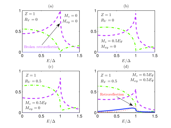
Figure 2: (Color online). Plot of the probability coefficients associated with the scattering processes at the interface. For an electron with incoming spin $\sigma$, the green (dash-dotted) line corresponds to normal reflection with spin $\sigma$, the magenta (dashed) line corresponds to Andreev-reflection of a hole with spin $-\sigma$, the blue (full) line designates reflection without branch-crossing with spin $-\sigma$, while the presence of retroreflection, i.e. Andreev-reflection of a hole with spin $\sigma$, is indicated by the red (dotted) line. Note from (d) that in order to get retroreflection, both an in-plane magnetization and a spin-active barrier is required.

To investigate how large the magnitude of the retroreflection coefficient may become, possibly even outgrowing the probability for ”normal” Andreev-reflection, we plotted the case of zero net polarization for several values of $M_{xy}$ in Fig. 3. It is seen that as $M_{xy}$ increases, the probability for retroreflection grows, and eventually becomes much larger than the probability for ordinary Andreev-reflection. Thus, for a tunneling junction with a barrier that discriminates significantly between spin-$\uparrow$ and spin-$\downarrow$ electrons, the presence of spin-flip processes may induce a substantial modification to the traditional picture of broken retroreflection.

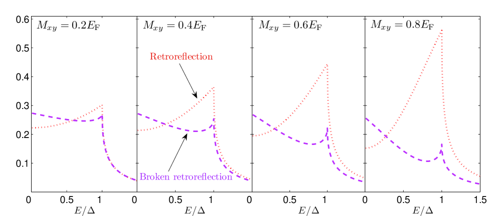
Figure 3: (Color online). Plot of probability coefficients for $Z=1$ and $R_{V}=0.95$ in the absence of any net polarization for several values of $M_{xy}$. It is seen that for increasing $M_{xy}$, i.e. larger effect of spin-flip scattering, the retroreflection process dominates the ”normal” Andreev-reflection.

Having established the presence of retroreflection, the next step is the consideration of how retroreflection leaves its signatures in experimentally measurable quantities. In this paper, we investigate how the presence of retroreflection may leave an experimental signature manifested in the conductance spectrum of a F/S junction. Although this shall be our focus, we note in passing that the reflection coefficients derived in Appendix A may also be used for the purpose of obtaining the current-voltage characteristics, spin-current, and spin conductance of the F/S junction. Normally, the charge- and spin-current may be written as

$$j_{\text{charge}}=-e\sum_{\sigma}j^{\sigma},\;j_{\text{spin}}=\sum_{\sigma}\sigma j^{\sigma},$$ (10)

where $j^{\sigma}$ is the particle-current of electrons with spin $\sigma$ over the interface. However, in the presence of spin-flip scattering, defining a proper spin-current requires a more careful analysis shi . One can always write down a well-defined spin-current in terms of physical spin-transport across the junction, but it may be very hard to experimentally distinguish whether the spin accumulation on either side of the interface should be attributed to physical spin transport or local spin-flip processes. The latter are present in e.g. systems with significant spin-orbit coupling or an in-plane magnetic field with respect to the quantization axis, which results in scattering between the two spin bands. Accordingly, in this paper we will concern ourselves with the charge-current and the resulting conductance spectrum.

IV Results

In our theory, we have included the possibility of having a spin-active barrier, Fermi-vector mismatch, arbitrary strength of the exchange energy on the F side, and different effective masses in the two systems. Thus, we believe our model should be able to capture many essential and realistic features of a F/S junction that pertain to both interfacial properties as well as bulk effects on the F and S side, respectively. Since the case of easy-axis magnetization has been thoroughly investigated, we shall be mainly concerned with the presence of retroreflection, which requires both spin-flip processes and a barrier acting as a spin-filter.
The single-particle tunneling conductance may be calculated by using the BTK-formalism btk , and reads

$$G(E) =\sum_{\sigma}G^{\sigma}(E),$$

$$G^{\sigma}(E) =\int^{\pi/2}_{-\pi/2}\text{d}\theta\cos\theta P^{\sigma}G^{\sigma}(E,\theta),$$

$$G^{\sigma}(E,\theta) =G_{N}^{-1}[1+R_{h}^{\uparrow}(E,\theta)+R_{h}^{\downarrow}(E,\theta)$$

$$\;\;-R_{e}^{\uparrow}(E,\theta)-R_{e}^{\downarrow}(E,\theta)],$$

$$G_{N} =\int^{\pi/2}_{-\pi/2}\text{d}\theta\cos\theta\frac{4\cos^{2}\theta}{4\cos^{2}\theta+Z^{2}},$$ (11)

where $Z=2m_{\text{F}}V/k_{F}$ and $G_{N}$ is the tunneling conductance for a N/N junction. Note that r.h.s. of the equation for $G^{\sigma}(E,\theta)$ appears to be independent of $\sigma$. However, it is implicitly understood in this notation that the reflection coefficients appearing on the r.h.s. have been solved for an incoming electron with spin $\sigma$, and these differ in the cases $\sigma=\uparrow$ and $\sigma=\downarrow$ since the wavefunction is different [see Eq. (II)]. The different probabilities for having spin injection $\sigma$ in the presence of a net polarization is accounted for by the factor $P^{\sigma}=(1+\sigma M_{Z}/E_{F})/2$. The quantities $\{R_{h}^{\sigma},R_{e}^{\sigma}\}$ are the probability coefficients for normal- and Andreev-reflection, and will be derived below. Note that these are not in general equal to the square amplitude of the scattering coefficients, and in particular not so in this case. To see this, consider the current-density of probability $\mathbf{J}_{\text{inc}}$ that is incident on the barrier,

$$\mathbf{J}_{\text{inc}}=\frac{1}{2m_{\text{F}}\mathrm{i}}(\psi^{*}\nabla\psi-\psi\nabla\psi^{*}),$$ (12)

obeying the conservation law

$$\frac{\partial P}{\partial t}+\nabla\cdot\mathbf{J}_{\text{inc}}=0.$$ (13)

Here, $P=|\psi|^{2}$. Consulting Eq. (II) and extracting the part of $\psi$ that corresponds to the incident wave-function, one readily obtains

$$\mathbf{J}_{\text{inc}}=\frac{\cos\theta}{m_{\text{F}}}(s_{\uparrow}k^{\uparrow}+s_{\downarrow}k^{\downarrow})\hat{\mathbf{x}}.$$ (14)

Since probability must be conserved, we have

$$\mathbf{J}_{\text{inc}}=-\mathbf{J}_{\text{refl}}+\mathbf{J}_{\text{trans}},$$ (15)

where the reflected probability current-density reads

$$\mathbf{J}_{\text{refl}} =\frac{1}{2m_{\text{F}}\mathrm{i}}[(\psi_{e}^{*}\nabla\psi_{e}-\text{h.c.})-(\psi_{h}^{*}\nabla\psi_{h}-\text{h.c.})],$$

$$\psi_{e} =r_{e}^{\uparrow}\begin{pmatrix}a\\ b\mathrm{e}^{-\mathrm{i}\phi}\\ \end{pmatrix}\mathrm{e}^{-\mathrm{i}k^{\uparrow}Sx}+r_{e}^{\downarrow}\begin{pmatrix}-b\mathrm{e}^{\mathrm{i}\phi}\\ a\\ \end{pmatrix}\mathrm{e}^{-\mathrm{i}k^{\downarrow}\tilde{S}x},$$

$$\psi_{h} =r_{h}^{\uparrow}\begin{pmatrix}a\\ b\mathrm{e}^{\mathrm{i}\phi}\\ \end{pmatrix}\mathrm{e}^{\mathrm{i}k^{\uparrow}Sx}+r_{h}^{\downarrow}\begin{pmatrix}-b\mathrm{e}^{-\mathrm{i}\phi}\\ a\\ \end{pmatrix}\mathrm{e}^{\mathrm{i}k^{\downarrow}\tilde{S}x}.$$ (16)

The opposite signs of the electron- and hole-part of $\psi$ entering $\mathbf{J}_{\text{refl}}$ pertain to the fact that their energy eigenvalues have opposite signs, as one may infer from the BdG-equations that are used to derive the explicit expression for $\mathbf{J}_{\text{refl}}$ from Eq. (15). One finds that

$$\mathbf{J}_{\text{refl}}=-\frac{1}{m_{\text{F}}}[k^{\uparrow}S|r_{e}^{\uparrow}|^{2}+k^{\uparrow}S|r_{h}^{\uparrow}|^{2}+k^{\downarrow}\tilde{S}|r_{e}^{\downarrow}|^{2}+k^{\downarrow}\tilde{S}|r_{h}^{\downarrow}|^{2}]\hat{\mathbf{x}}.$$ (17)

The same procedure may now be applied to $\mathbf{J}_{\text{trans}}$, such that Eq. (15) can be written as

$$1=\sum_{\sigma}(R_{e}^{\sigma}+R_{h}^{\sigma}+T_{e}^{\sigma}+T_{h}^{\sigma})$$ (18)

upon division with $|\mathbf{J}_{\text{inc}}|$. From this, one infers that

$$R_{e}^{\uparrow} =|r_{e}^{\uparrow}|^{2}\frac{k^{\uparrow}S}{s_{\uparrow}k^{\uparrow}\cos\theta+s_{\downarrow}k^{\downarrow}\cos\theta},$$

$$R_{e}^{\downarrow} =|r_{e}^{\downarrow}|^{2}\frac{k^{\downarrow}\tilde{S}}{s_{\uparrow}k^{\uparrow}\cos\theta+s_{\downarrow}k^{\downarrow}\cos\theta},$$

$$R_{h}^{\uparrow} =|r_{h}^{\uparrow}|^{2}\frac{k^{\uparrow}S}{s_{\uparrow}k^{\uparrow}\cos\theta+s_{\downarrow}k^{\downarrow}\cos\theta},$$

$$R_{h}^{\downarrow} =|r_{h}^{\downarrow}|^{2}\frac{k^{\downarrow}\tilde{S}}{s_{\uparrow}k^{\uparrow}\cos\theta+s_{\downarrow}k^{\downarrow}\cos\theta}.$$ (19)

The coefficients $\{R_{e}^{\sigma},R_{h}^{\sigma},T_{e}^{\sigma},T_{h}^{\sigma}\}$ have the status of probability coefficients for their respective processes, and obey the conservation law Eq. (18). Note that in the absence of exchange splitting, i.e. F$\to$ N and $\theta_{A}=\theta$, one obtains $R_{i}^{\sigma}=|r_{i}^{\sigma}|^{2}$.

IV.1 Effect of Fermi-vector mismatch

To account for the Fermi-vector mismatch, we introduce a parameter $R_{E}=E_{\text{S}}/E_{\text{F}}$. This allows the Fermi energies in the F and S regions to be different, which effectively models unequal carrier densities and bandwidths on each side of the junction. For ferromagnet/high-$T_{c}$ superconductor junctions, an appropriate choice appears to be zutic00 $R_{E}\leq 1$. In our study, however, we will consider values of $R_{E}$ both less than and greater than unity. To begin with, we fix the strength of the planar contribution to the exchange energy at $M_{xy}=0.1E_{F}$ and set $M_{z}=0$, plotting the conductance spectrum for several values of $R_{E}$. We fix the ratio $R_{V}=V_{s}/V_{0}=0.5$, such that the conditions for retroreflection are fulfilled. For each figure, we consider zero ($Z=0$), weak ($Z=1$), and large ($Z=10$) interfacial resistance; $Z=0$ corresponds to the point-contact (also called metallic contact, in some literature) while $Z\to\infty$ equivalents the tunneling limit. The conductance spectrum for weak spin-flip scattering ($M_{xy}=0.1E_{F}$) and $M_{z}=0$ with $R_{V}=0.5$ for several values of $Z$, is depicted in Fig. 4. From Fig. 4, we infer that the conductance behaves in a monotonic way upon variation of $R_{E}$, and that the conductance is suppressed with decreasing $R_{E}$.

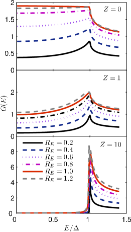
Figure 4: (Color online). Conductance spectrum for weak spin-flip scattering ($M_{xy}=0.1E_{F}$) and $M_{z}=0$ with $R_{V}=0.5$ for several values of $Z$.

Next, we increase the exchange energy to $M_{xy}=0.5E_{F}$ and set $R_{V}=0.95$ such that spin-flip processes become more dominant and the barrier discriminates strongly between spin-$\uparrow$ and spin-$\downarrow$ electrons. The resulting $G(E)$ is illustrated in Fig. 5, where it is seen that a nonmonotonic behaviour appears. Specifically, the peak at $E=\Delta$ vanishes for $R_{E}\simeq 1$, as is most clearly seen for the case of large interfacial resistance.

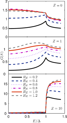
Figure 5: (Color online). Conductance spectrum for strong spin-flip scattering ($M_{xy}=0.5E_{F}$) and $M_{z}=0$ with a strongly spin-dependent barrier ($R_{V}=0.95$) for several values of $Z$.

One of the results of Refs. zutic99, ; zutic00, was that the effect of Fermi-vector mismatch yielded an increased subgap conductance when there was a net spin-polarization. As an important consequence, this finding suggested that the interfacial barrier parameter $Z$ was not sufficient to account for the conductance features in the presence of both spin polarization and Fermi-vector mismatch, since the increase of subgap conductance could not be reproduced by varying $Z$ alone. In Figs. 4 and 5, no such increase in subgap conductance was found, but these correspond to an unpolarized case since $M_{z}=0$. In order to investigate how the spin-flip scattering and spin-active barrier affects this particular feature of the Fermi-vector mismatch, we plot the normal incidence $\theta=0$ conductance $G(E,\theta=0)$ for the same parameters as Fig. 1 in Refs. zutic99, ; zutic00, for the sake of direct comparison. Note that due to a different scaling of the conductance to make it dimensionless, the quantitative results for $G(E,\theta=0)$ is not the same as the result in Refs. zutic99, ; zutic00, , although the qualitative aspect is identical. This is because we scale the conductance on $G_{N}$ given by Eq. (IV) For $Z=0$, this merely amounts to a factor of 2. In the upper panel of Fig. 6, we reproduce Fig. 1b of Ref. zutic00, to illustrate our consistency with their results. Note that the parameter $L_{0}^{2}$ in Ref. zutic00, is equivalent to our $R_{E}$ when $R_{m}=1$, i.e. the effective masses are the same. The middle panel now includes spin-flip scattering with $M_{xy}=0.4E_{F}$, while $Z=0$. The lower panel shows the combined effect of planar magnetization and a spin-active barrier, resulting in triplet correlations, with $M_{xy}=0.4E_{F}$ and $\{Z=1,R_{V}=0.95\}$. It is seen that the qualitative change is most dramatic when the conditions for retroreflection are fulfilled.

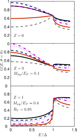
Figure 6: (Color online). Conductance spectrum for zero spin-flip scattering and purely non-magnetic scattering potential (upper panel), spin-flip scattering and purely non-magnetic scattering potential (middle panel), spin-flip scattering and mixed magnetic/non-magnetic scattering potential. For all panels, $M_{z}/E_{F}=0.866$ for comparison with Ref. zutic00, . The lines are given at $E=1.4$ for the upper panel as follows (from top to bottom): $R_{E}=\{1,1/\sqrt{2},1/2,1/4,1/9,1/16\}$.

IV.2 Effect of exchange energy

We now proceed to consider how the strength of the exchange energy, both planar ($M_{xy}$) and easy-axis ($M_{z}$), affects the conductance spectrum. We set the masses and Fermi energies to be equal in the F and S part of the system, and study how the angularly averaged $G(E)$ is affected by increasing $M_{Z}$ for a given $M_{xy}$. Let us first set $M_{xy}=0.1E_{F}$ and $R_{V}=0.5$, as shown in Fig. 7. In accordance with our previous observation that Andreev-reflection is inhibited by a net polarization in the F part of the system, it is seen that the conductance is suppressed with increasing $M_{z}$. However, in the lower panel of Fig. 7 where the tunneling limit of the junction is considered, the conductance increases with $M_{z}$ for $E>\Delta$.

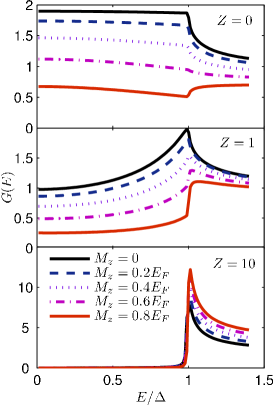
Figure 7: (Color online). Conductance spectra for various non-magnetic scattering potentials upon varying the polarization of the ferromagnet with $M_{xy}=0.1E_{F}$ and $R_{V}=0.5$.

Increasing the strength of the spin-flip scattering and also the spin-dependence of the barrier, the resulting conductance spectra are shown in Fig. 8 with $M_{xy}=0.5E_{F}$ and $R_{V}=0.95$. The general effect of optimizing the conditions for the presence of retroreflection processes seems to be a ”smoothing out” of the conductance: the sharp features at $E=\Delta$ become blunt, an observation which is most clearly revealed in the tunneling limit. As an experimental consequence, the nature of the features at $E=\Delta$ in the case of a high-resistance interface could thus offer information concerning to what degree retroreflection is present in the system.

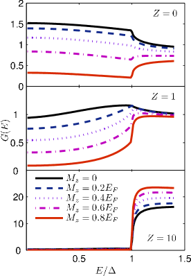
Figure 8: (Color online). Conductance spectra for various non-magnetic scattering potentials upon varying the polarization of the ferromagnet with $M_{xy}=0.5E_{F}$ and $R_{V}=0.95$.

IV.3 Effect of different effective masses

To investigate the effect of different effective masses in the F and S part of the system, we consider three ratios: $R_{m}=m_{\text{S}}/m_{\text{F}}\in\{0.01,0.1,1\}$. In Fig. 9, we have plotted the case of weak spin-flip scattering and a moderate spin-dependence of the barrier, while in Fig. 10 we investigate significant spin-flip scattering and a strongly spin-dependent interfacial resistance. In the first case, decreasing $R_{m}$ clearly inhibits the tunneling conductance with no exotic features present except the usual peak at $E=\Delta$. In the tunneling limit, it is interesting to observe that only in the case $R_{m}=1$ is the maximum of the conductance located at $E=\Delta$. Upon decreasing $R_{m}$, one sees that the characteristic peak of the spectrum is translated to lower energies and that it becomes less sharp. There is still a sudden increase of current at $E=\Delta$, manifested as a jump in the conductance spectrum, but it is less protruding for lower ratios of $R_{m}$ than unity.

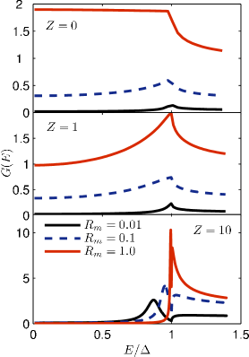
Figure 9: (Color online). Conductance spectra for different effective masses with parameters $M_{xy}=0.1E_{F}$ and $R_{V}=0.5$.

When the conditions for retroreflection become more pronounced, as is the case in Fig. 10, one may again observe the general modification of the conductance to a more featureless curve in the case of no barrier and a weak barrier ($Z=1$), as was the case in the previous subsection. In the tunneling limit, the presence of retroreflection also modifies the spectra such that the sharp peak is lost at the gap energy, although the sudden jump due to the initiated flow of current at $E=\Delta$ is still there.

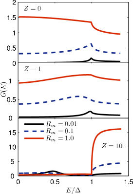
Figure 10: (Color online). Conductance spectra for different effective masses with parameters $M_{xy}=0.5E_{F}$ and $R_{V}=0.95$.

IV.4 Effect of magnetic and non-magnetic scattering potential

In this section, we show that the conductance spectrum may reveal clear-cut signatures of the presence of retro-reflection as a result of the interplay between $V_{0}$ and $V_{s}$ when $M_{xy}\neq 0$. We keep the latter fixed at $M_{xy}=0.5E_{F}$, and plot $G(E)$ for $Z\in\{0.1,1,5\}$ while varying the strength of the magnetic scattering potential. From Fig. 11, we see that at $Z=0.1$, the presence of retro-reflection is very weak and the conductance spectrum remains virtually unaltered as $V_{s}$ is varied. At $Z=1$, the effect of increasing the strength of the magnetic potential of the barrier, acting as a spin-filter, corresponds to a reduction of the conductance-peak at $E=\Delta$. This is in agreement with our previous observations that the presence of retroreflection appears to have a smoothing effect on the conductance spectrum, causing it to soften its characteristic features. At $Z=5$, the crossover from a sharp peak at $E=\Delta$ at small $R_{V}$ to a ”waterfall”-shape for large $R_{V}$ is clearly illustrated. We suggest that this signature could be used as a feature that unveils the presence of retroreflected holes in the system, and thus indicates triplet correlations due to the interplay between spin-flip processes and a barrier acting as a spin-filter.

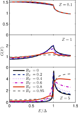
Figure 11: (Color online). Conductance spectra in the presence of retroreflection but in the absence of any net polarization. Here, $M_{xy}=0.5E_{F}$ while $M_{Z}=0$.

To investigate how a net polarization will affect the conductance spectra in this case, consider Fig. 12 which illustrates the conductance for the same parameters as in Fig. 11 except that now $M_{z}=0.5E_{F}$. In agreement with previous remarks, the conductance suffers a general reduction due to the net polarization in the upper and lower panel. However, the conductance corresponding to the strongest polarization comes out on top in the tunneling limit as in the case of Fermi-vector mismatch. Apart from this, the same features as in Fig. 11 are present, with retroreflection leaving its fingerprint most obviously in the behaviour of the conductance at $E=\Delta$ in the tunneling limit.

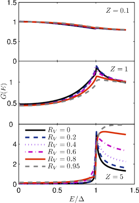
Figure 12: (Color online). Conductance spectra in the presence of retroreflection and a net polarization. Here, $M_{xy}=0.5E_{F}$ while $M_{Z}=0.5E_{F}$.

V Discussion

We have shown that the presence of a spin-active barrier combined with a planar component of the magnetization in the F induces new features in the proximity effect in a F/S junction. Physically, this may be understood by realizing that only an $S_{z}=0$ triplet component is induced for a spin-active barrier in the absence of spin-flip processes near the junction, while the equal-spin $(S_{z}=\pm 1)$ triplet components are generated only if a spin-flip potential is also present. On the other hand, spin-flip processes alone in the absence of a spin-active barrier would inhibit singlet pairing without generating any triplet components. An interesting opportunity that arises due to the restoration of retro-reflection is the fact that one may generate currents with a varying degree of spin-polarization in the F part. In the conventional case, an incident electron with spin $\sigma$ is reflected as either an electron with spin $\sigma$ or hole with spin $-\sigma$ in these systems. In the present case, however, the reflected electrons and holes may carry either $\uparrow$ and $\downarrow$ spin, depending on parameters such as the magnitude of the exchange energy and the intrinsic/spin-dependent barrier strength. In principle, it could possible to generate pure spin-currents without charge-currents and vice versa as a result of the additional allowed spin state of the reflected holes and electrons. It is also intriguing to observe that due to the coupling between $\phi$ and $\gamma$, it may be possible to obtain a Josephson current in a S/F/S hybrid structure that is sensitive to a rotation of the magnetization in the ferromagnetic part, which has been recently discussed in Refs. kreuzy, ; pajovic, .
It was shown in Ref. bergeretPRL, that if a local inhomogeneity of the magnetization in the vicinity of a F/S interface was present, a spin-triplet component of the S order parameter will be generated and penetrate into the F much deeper than the spin-singlet component. In a S/half-metal/S junction, it has been found that S triplet correlations would be induced on both sides of the junctions in the presence of spin-mixing and spin-flip scattering at the interfaces eschrigPRL (see also Ref. tokuyasu, ). We have found that spin-triplet pairing correlations may be induced in the presence of a spin-active barrier, i.e. intrinsic spin-mixing at the interface, and a planar magnetization relative to the quantization axis. It seems reasonable to suggest that these findings are closely related to the conditions put forward by Ref. eschrigPRL, , since planar magnetization components may effectively act as a spin-flip scattering potential. Our results are thus consistent with the findings of recent studies, although we have adressed several new aspects of the scattering problem in the present paper. In particular, we have found an interplay between in-plane magnetization direction and superconducting phase which to our knowledge has not been investigated before. Moreover, we compute detailed conductance spectra of the F/S junction under many different conditions.
One of the important findings of Refs. zutic99, ; zutic00, was that a zero-bias conductance peak (ZBCP) would develop under the right conditions in the F/S junction, and the effect was attributed to the influence of Fermi-vector mismatch. Usually, the appearance of a ZBCP is associated with unconventional superconductivity where it may appear due to the different phases felt by the transmitted electron-like and hole-like quasiparticles in the superconductor tanaka . However, Zutic and Valls zutic99 ; zutic00 showed that no unconventional superconductivity was required to obtain a ZBCP, and that the effect of Fermi-vector mismatch in a F/S junction thus offered a different mechanism for the formation of a ZBCP than the usual one, attributed to a $\mathbf{k}$-dependent gap. However, it should be noted that the ZBCP obtained in Refs. zutic99, ; zutic00, is not as sharp (delta-function like) as the ZBCP depicted in e.g. Ref. tanaka, , where unconventional superconductors (high $T_{c}$ $d$-wave, to be specific) were considered.
In the present paper, we consider a more general situation than Zutic and Valls, allowing for a completely arbitrary magnetization direction and a spin-active barrier. As we have shown, this changes the physical picture dramatically and opens up a new transport channel for both charge and spin, namely retroreflected holes. For consistency, we show that we are able to completely reproduce Fig. 3 of Ref. zutic00, , where the conductance for normal incidence $\theta=0$ is presented (our Fig. 13).

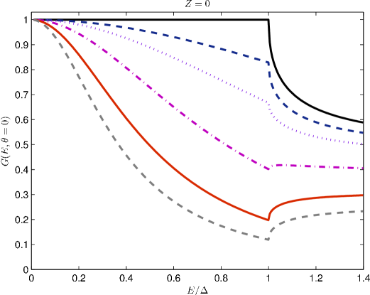
Figure 13: (Color online). In the limit $M_{xy}\to 0$, the formation of a ZBCP is observed with decreasing $R_{E}$. This illustrates how the effect of Fermi-vector mismatch may ”mimick” the usual signature of unconventional superconductivity, namely the appearance of a ZBCP for certain crystal orientations. This was first discussed in Ref. zutic00, , see their Fig. 3. From top to bottom, the curves correspond to the following pairs of $(R_{E},M_{z}/E_{F})$: (1,0), $(\frac{1}{\sqrt{2}},\frac{1}{\sqrt{2}})$, $(\frac{1}{2},0.866)$, $(\frac{1}{4},0.968)$, $(\frac{1}{9},0.994)$, and $(\frac{1}{16},0.998)$.

In contrast to Zutic and Vallszutic00 , due to the unwieldy expressions for the reflection coefficients (see Appendix A), we are not able to give analytically the condition that yields the largest value of the conductance at zero-bias [cf. their Eq. (3.4)]. It is thus not straight-forward to identify the proper parameter regime that would yield the maximum value of $G(0)$. We therefore leave the question concerning how spin-flip scattering and a spin-active barrier affect the formation of a ZBCP in a F/S-junction, as open.
Scattering on the barrier leads to a suppression of the S order parameter close [of order coherence length, ${\cal{O}}(\xi)$] to the junction. For a weakly polarized ferromagnet, we expect that inclusion of a spatial variation of the order parameter does not change our results qualitatively, since it is well-known that the approximation of a constant order parameter up to the junction is excellent in a N/$s$-wave superconductor junction (see e.g. Ref. bruder, ). For a strongly polarized ferromagnet, the superconducting singlet order parameter may however be suppressed significantly in the vicinity of the gap eschrigPRL . For unconventional pairing symmetries ($d$-wave), it was shown in Ref. tanaka2000, that the effect of taking into account the suppression of the order parameter in the presence of Andreev bound surface states remains almost unchanged around zero bias voltage, although a broadening of the ZBCP is observed. Since no zero energy surface states are present for a pure $s$-wave singlet component of the superconducting order parameter, we believe that our approximation of a step-function $\Delta$ should be justified.
It is worth noting that a F/S junction as considered here with a spin-active barrier is in some respects similar to previously studied F/F/S junctions kikuchi if the magnetization directions of the two F layers are non-collinear. While Ref. kikuchi, considers the conductance spectrum in the case of collinear magnetization directions of the F layers, a previous study kopu has developed a quite general framework for dealing with F/S junctions by introducing a phenomenological spin-mixing angle which describes a spin-active interface. In Ref. kopu, , the conductance is explicitly calculated for a half-metallic ferromagnet/$s$-wave superconductor junction. In the present paper, we have developed a similar framework for treating F/S junctions with a spin-active interface, but using a different formalism. Our theory allows for describing a very wide range of physical phenomena, such as arbitrary magnetization strength/direction of the ferromagnet, a spin-active barrier, Fermi-vector mismatch, and different effective masses in the two systems. We have explicitly computed the conductance spectra for the metallic case with non-collinear magnetizations between the F-part and the spin-active barrier in a F/S system. Hence, our work expands on the results of Ref. kikuchi, and Ref. kopu, , and we reproduce their results in the appropriate limits.
The similarity of our model with F/F/S junction with noncollinear magnetizations may be understood by realizing that using a spin basis that diagonalizes the scattering matrix of one ferromagnet will cause the magnetization in the other ferromagnet to effectively look like a spin flip term and vice versa. Although this analogy could be of some use for comparing the present system under consideration with F/F/S junctions, it should not be taken too far since in our case we are dealing with an insulating, very thin barrier with both magnetic and non-magnetic scattering potentials as opposed to a conducting ferromagnetic layer.
Another issue that deserves mentioning is that the magnetic field due to the magnetization of the F will penetrate into the thin-film structure of the S along the plane. An in-plane magnetic field may actually coexist uniformly meservey with $s$-wave S in a thin-film (in contrast to the bulk case varma ; shen ) and effects such as orbital pair-breaking or formation of vortices will be prohibited as long as the thickness $t$ of the film is less than both $\lambda$ and $\xi_{0}$. It is also reasonable to neglect any exchange interactions in the S since the induced field due to the magnetization is much smaller [of order ${\cal{O}}$($10^{-3}$)] than the exchange field in the F, and can thus be safely neglected buzdinRMP . Moreover, we stress that the clean limit has been considered in the present paper, which hopefully provides an initial idea of the physics that can be expected when the effect of disorder is included in the system, although this requires a separate analysis.

VI Summary

In this paper, we have presented a detailed investigation of the conductance spectra of a F/S junction, expanding previous work substantially by allowing for a completely arbitrary direction of magnetization, which effectively accounts for spin-flip scattering due to a planar component of the magnetization, and a spin-active barrier. Our procedures amounts to an extension of the BTK-formalism, along the lines of several other workers (e.g. tanaka ; kashiwaya1999 ), and have given us the advantadge of obtaining analytical solutions, primarily due to the step-function approximation for the superconducting and magnetic order parameters.
From our results, one may infer that several new qualitative features arise due to the presence of spin-flip scattering and a spin-active barrier. We demonstrate the re-entrance of retroreflection for the Andreev-reflected hole, which is absent for an easy-axis ferromagnet with a purely non-magnetic interfacial scattering potential. This opens up a new transport channel for both spin and charge, and is interpreted as a signature of spin-triplet correlations in the system. In this context, a most interesting interplay between the superconducting phase $\gamma$ and the planar magnetization orientation characterized by the azimuthal angle $\phi$ arises in the phase coherence of retroreflected holes. This particular feature may be exploited in terms of a Josephson current in a S/F/S junction that responds to a rotation of $\phi$.
As our main result, we have investigated the influence on the conductance spectra due to different effective masses, Fermi-vector mismatch, strength of the exchange energy, and the influence of varying the relative strength of magnetic and non-magnetic scattering in the F/S junction. Our findings are consistent with those of Ref. zutic00, with respect to the observation of an increased subgap conductance for increasing Fermi-vector mismatch for a large spin polarization. In the presence of a spin-active barrier, however, this effect vanishes. The general influence of retroreflection on the conductance spectra seems to be a softening of the sharp features such as peaks and dips at $E=\Delta$. Also, as a signature which should be clearly discernable experimentally, a crossover from peak to ”waterfall” shape takes place in the tunneling limit at the gap energy.
We believe that our angle of approach for treating the F/S junction in the extended BTK-formalism should suffice to shed light on the rich physics and concomitant important phenomena that are present in such systems, which is of particular relevance in the context of spin polarized tunneling spectroscopy.

Appendix A Derivation of scattering coefficients

From the boundary conditions, the condition of continuity of the wave-function yields the expressions

$$s_{\uparrow}a-s_{\downarrow}b\mathrm{e}^{-\mathrm{i}\phi}+r_{e}^{\uparrow}-r_{e}^{\downarrow}b\mathrm{e}^{\mathrm{i}\phi}=t_{e}^{\uparrow}u+t_{h}^{\downarrow}v\mathrm{e}^{\mathrm{i}\gamma},$$

$$s_{\uparrow}b\mathrm{e}^{-\mathrm{i}\phi}+s_{\downarrow}a+r_{e}^{\uparrow}b\mathrm{e}^{-\mathrm{i}\phi}+r_{e}^{\downarrow}a=t_{e}^{\downarrow}u-t_{h}^{\uparrow}v\mathrm{e}^{\mathrm{i}\gamma}$$

$$r_{h}^{\uparrow}a-r_{h}^{\downarrow}b\mathrm{e}^{-\mathrm{i}\phi}=-t_{e}^{\downarrow}v\mathrm{e}^{-\mathrm{i}\gamma}+t_{h}^{\uparrow}u,$$

$$r_{h}^{\uparrow}b\mathrm{e}^{\mathrm{i}\phi}+r_{h}^{\downarrow}a=t_{e}^{\uparrow}v\mathrm{e}^{-\mathrm{i}\gamma}+t_{h}^{\downarrow}u,$$ (20)

while the matching of derivatives at $x=0$ yields

$$(V_{0}-V_{s})(t_{e}^{\uparrow}u+t_{h}^{\downarrow}v\mathrm{e}^{\mathrm{i}\gamma})=\frac{\mathrm{i}q\cos\theta_{s}}{2m_{\text{S}}}(ut_{e}^{\uparrow}-v\mathrm{e}^{\mathrm{i}\gamma}t_{h}^{\downarrow})$$

$$-\frac{\mathrm{i}}{2m_{\text{F}}}[\cos\theta(k^{\uparrow}s_{\uparrow}a-k^{\downarrow}s_{\downarrow}b\mathrm{e}^{\mathrm{i}\phi})-k^{\uparrow}Sar_{e}^{\uparrow}+k^{\downarrow}\tilde{S}b\mathrm{e}^{\mathrm{i}\phi}r_{e}^{\downarrow}],$$

$$(V_{0}+V_{s})(t_{e}^{\downarrow}u-t_{h}^{\uparrow}v\mathrm{e}^{\mathrm{i}\gamma})=\frac{\mathrm{i}q\cos\theta_{s}}{2m_{\text{S}}}(ut_{e}^{\downarrow}+v\mathrm{e}^{\mathrm{i}\gamma}t_{h}^{\uparrow})$$

$$-\frac{\mathrm{i}}{2m_{\text{F}}}[\cos\theta(k^{\uparrow}s_{\uparrow}b\mathrm{e}^{-\mathrm{i}\phi}+k^{\downarrow}s_{\downarrow}a)-k^{\uparrow}Sb\mathrm{e}^{-\mathrm{i}\phi}r_{e}^{\uparrow}-k^{\downarrow}\tilde{S}ar_{e}^{\downarrow}],$$

$$(V_{0}-V_{s})(-t_{e}^{\downarrow}v\mathrm{e}^{-\mathrm{i}\gamma}+t_{h}^{\uparrow}u)=-\frac{\mathrm{i}q\cos\theta_{s}}{2m_{\text{S}}}(v\mathrm{e}^{-\mathrm{i}\gamma}t_{e}^{\downarrow}+ut_{h}^{\uparrow})$$

$$-\frac{\mathrm{i}}{2m_{\text{F}}}(k^{\uparrow}Sar_{h}^{\uparrow}-k^{\downarrow}\tilde{S}b\mathrm{e}^{-\mathrm{i}\phi}r_{h}^{\downarrow}),$$

$$(V_{0}+V_{s})(t_{e}^{\uparrow}v\mathrm{e}^{-\mathrm{i}\gamma}+t_{h}^{\downarrow}u)=\frac{\mathrm{i}q\cos\theta_{s}}{2m_{\text{S}}}(t_{e}^{\uparrow}v\mathrm{e}^{-\mathrm{i}\gamma}-t_{h}^{\downarrow}u)$$

$$-\frac{\mathrm{i}}{2m_{\text{F}}}(k^{\uparrow}Sb\mathrm{e}^{\mathrm{i}\phi}r_{h}^{\uparrow}+k^{\downarrow}\tilde{S}ar_{h}^{\downarrow}).$$ (21)

Solving for the transmission coefficients, one is left with the reduced set of equations

$$t_{e}^{\uparrow}A_{1}+t_{e}^{\downarrow}B_{1}\mathrm{e}^{\mathrm{i}\phi}+t_{h}^{\uparrow}C_{1}\mathrm{e}^{\mathrm{i}(\phi+\gamma)}+t_{h}^{\downarrow}D_{1}\mathrm{e}^{\mathrm{i}\gamma} =X_{1},$$

$$t_{e}^{\uparrow}A_{2}\mathrm{e}^{-\mathrm{i}\phi}+t_{e}^{\downarrow}B_{2}+t_{h}^{\uparrow}C_{2}\mathrm{e}^{\mathrm{i}\gamma}+t_{h}^{\downarrow}D_{2}\mathrm{e}^{\mathrm{i}(\gamma-\phi)} =X_{2},$$

$$t_{e}^{\uparrow}A_{3}\mathrm{e}^{-\mathrm{i}(\phi+\gamma)}+t_{e}^{\downarrow}B_{3}\mathrm{e}^{-\mathrm{i}\gamma}+t_{h}^{\uparrow}C_{3}+t_{h}^{\downarrow}D_{3}\mathrm{e}^{-\mathrm{i}\phi} =0,$$

$$t_{e}^{\uparrow}A_{4}\mathrm{e}^{-\mathrm{i}\gamma}+t_{e}^{\downarrow}B_{4}\mathrm{e}^{\mathrm{i}(\phi-\gamma)}+t_{h}^{\uparrow}C_{4}\mathrm{e}^{\mathrm{i}\phi}+t_{h}^{\downarrow}D_{4} =0.$$ (22)

From Eqs. (A), one finds that

$$t_{h}^{\downarrow} =X_{1}F_{1}\mathrm{e}^{-\mathrm{i}\gamma}+X_{2}F_{2}\mathrm{e}^{\mathrm{i}(\phi-\gamma)},$$

$$t_{h}^{\uparrow} =X_{2}R_{1}\mathrm{e}^{-\mathrm{i}\gamma}+R_{e}t_{h}^{\downarrow}\mathrm{e}^{-\mathrm{i}\phi},$$

$$t_{e}^{\downarrow} =P_{1}t_{h}^{\uparrow}\mathrm{e}^{\mathrm{i}\gamma}+P_{2}t_{h}^{\downarrow}\mathrm{e}^{\mathrm{i}(\gamma-\phi)},$$

$$t_{e}^{\uparrow} =-(B_{4}t_{e}^{\downarrow}\mathrm{e}^{\mathrm{i}\phi}+C_{4}t_{h}^{\uparrow}\mathrm{e}^{\mathrm{i}(\phi+\gamma)}+D_{4}t_{h}^{\downarrow}\mathrm{e}^{\mathrm{i}\gamma})/A_{4},$$ (23)

such that the reflection coefficients $\{r_{h}^{\sigma},r_{e}^{\sigma}\}$ may be obtained by back-substitution of Eqs. (A) into Eqs. (A). We have defined the following auxiliary quantities:

$$X_{1} =\frac{1}{2m_{\text{F}}}(k^{\uparrow}\cos\theta s_{\uparrow}a-k^{\downarrow}\cos\theta s_{\downarrow}b\mathrm{e}^{\mathrm{i}\phi}$$

$$+k^{\uparrow}Sas_{\uparrow}-k^{\downarrow}\tilde{S}s_{\downarrow}\mathrm{e}^{\mathrm{i}\phi}),$$ (24)

$$X_{2} =\frac{1}{2m_{\text{F}}}(k^{\uparrow}\cos\theta b\mathrm{e}^{-\mathrm{i}\phi}+k^{\downarrow}\cos\theta s_{\downarrow}a$$

$$+k^{\uparrow}Ss_{\uparrow}\mathrm{e}^{-\mathrm{i}\phi}+k^{\downarrow}\tilde{S}s_{\downarrow}a),$$ (25)

$$F_{1} =[D_{1}+C_{1}R_{2}+P_{1}B_{1}R_{2}+B_{1}P_{2}$$

$$-\frac{A_{1}}{A_{4}}(B_{4}P_{2}+B_{4}P_{1}R_{2}+R_{2}C_{4}+D_{4})]^{-1},$$ (26)

$$F_{2} =F_{1}[\frac{A_{1}}{A_{4}}(B_{4}P_{1}R_{1}+R_{1}C_{4})-B_{1}P_{1}R_{1}-C_{1}R_{1}],$$ (27)

$$R_{1} =[C_{2}+B_{2}P_{1}-\frac{A_{2}}{A_{4}}(B_{4}P_{1}+C_{4})]^{-1},$$ (28)

$$P_{1} =(\frac{C_{4}A_{3}}{A_{4}}-C_{3})/(B_{3}-\frac{A_{3}B_{4}}{A_{4}}),$$ (29)

$$R_{2} =R_{1}[B_{2}P_{2}+D_{2}-\frac{A_{2}}{A_{4}}(B_{4}P_{2}+D_{4})],$$ (30)

$$P_{2} =(\frac{D_{4}A_{3}}{A_{4}}-D_{3})/(B_{3}-\frac{A_{3}B_{4}}{A_{4}}),$$ (31)

in addition to

$$A_{1} =\mathrm{i}(V_{0}-V_{s})u+\frac{1}{2m_{\text{S}}}q\cos\theta_{s}u+\frac{u}{2m_{\text{F}}}(k^{\uparrow}Sa^{2}+k^{\downarrow}\tilde{S}b^{2}),\;A_{2}=\frac{1}{2m_{\text{F}}}(k^{\uparrow}S-k^{\downarrow}\tilde{S})abu,$$ (32)

$$A_{3} =\frac{1}{2m_{\text{F}}}(k^{\downarrow}\tilde{S}-k^{\uparrow}S)abv,\;A_{4}=\mathrm{i}(V_{0}+V_{s})v+\frac{1}{2m_{\text{S}}}q\cos\theta_{s}v-\frac{v}{2m_{\text{F}}}(k^{\uparrow}Sb^{2}+k^{\downarrow}\tilde{S}a^{2}),$$ (33)

$$B_{1} =\frac{1}{2m_{\text{F}}}(k^{\uparrow}S-k^{\downarrow}\tilde{S})abu,\;B_{2}=\mathrm{i}(V_{0}+V_{s})u+\frac{1}{2m_{\text{S}}}q\cos\theta_{s}u+\frac{u}{2m_{\text{F}}}(k^{\uparrow}Sa^{2}+k^{\downarrow}\tilde{S}b^{2}),$$ (34)

$$B_{3} =-\mathrm{i}(V_{0}-V_{s})v-\frac{1}{2m_{\text{S}}}q\cos\theta_{s}v+\frac{v}{2m_{\text{F}}}(k^{\uparrow}Sa^{2}+k^{\downarrow}\tilde{S}b^{2}),\;B_{4}=-\frac{1}{2m_{\text{F}}}(k^{\downarrow}\tilde{S}-k^{\uparrow}S)abv,$$ (35)

$$C_{1} =\frac{1}{2m_{\text{F}}}(k^{\downarrow}\tilde{S}-k^{\uparrow}S)abv,\;C_{2}=-\mathrm{i}(V_{0}+V_{s})v+\frac{1}{2m_{\text{S}}}q\cos\theta_{s}v-\frac{v}{2m_{\text{F}}}(k^{\uparrow}Sb^{2}+k^{\downarrow}\tilde{S}a^{2}),$$ (36)

$$C_{3} =\mathrm{i}(V_{0}-V_{s})u-\frac{1}{2m_{\text{S}}}q\cos\theta_{s}u-\frac{u}{2m_{\text{F}}}(k^{\uparrow}Sa^{2}+k^{\downarrow}\tilde{S}b^{2}),\;C_{4}=-\frac{1}{2m_{\text{F}}}(k^{\uparrow}S-k^{\downarrow}\tilde{S})abu,$$ (37)

$$D_{1} =\mathrm{i}(V_{0}-V_{s})v-\frac{1}{2m_{\text{S}}}q\cos\theta_{s}v+\frac{v}{2m_{\text{F}}}(k^{\uparrow}Sa^{2}+k^{\downarrow}\tilde{S}b^{2}),\;D_{2}=\frac{1}{2m_{\text{F}}}(k^{\uparrow}S-k^{\downarrow}\tilde{S})abu,$$ (38)

$$D_{3} =\frac{1}{2m_{\text{F}}}(k^{\downarrow}\tilde{S}-k^{\uparrow}S)abu,\;D_{4}=\mathrm{i}(V_{0}+V_{s})u-\frac{1}{2m_{\text{S}}}q\cos\theta_{s}u-\frac{u}{2m_{\text{F}}}(k^{\uparrow}Sb^{2}+k^{\downarrow}\tilde{S}a^{2})$$ (39)

References

- (1) A. I. Buzdin, Rev. Mod. Phys. 77, 935-976 (2005).
- (2) I. O. Kulik, Sov. Phys. JETP 30, 944 (1970).
- (3) A. I. Buzdin, A. V. Vedyayev, and N. V. Ryzhanova, Europhys. Lett. 48, 686 (1999).
- (4) L. N. Bulaevskii, V. V. Kuzii, and A. A. Sobyanin, Pis ma Zh. Eksp. Teor. Fiz. 25, 314 (1977) [ JETP Lett. 25, 290 (1977)]; A. V. Andreev, A. I. Buzdin, and R. M. Osgood, Phys. Rev. B 43, 10124 (1991); F. S. Bergeret, A. F. Volkov, and K. B. Efetov, Phys. Rev. B 64, 134506 (2001).
- (5) V. V. Ryazanov, et al., Phys. Rev. Lett. 86, 2427 (2001); A. Bauer, et al., Phys. Rev. Lett. 92, 217001 (2004).
- (6) A. F. Andreev, Sov. Phys. JETP 19, 1228 (1964).
- (7) G. Deutscher, Rev. Mod. Phys. 77, 109 (2005).
- (8) M. Weides, M. Kemmler, H. Kohlstedt, A. Buzdin, E. Goldobin, D. Koelle, R. Kleiner, Appl. Phys. Lett. 89, 122511 (2006).
- (9) J. Y. T. Wei, N.-C. Yeh, D. F. Garrigus, and M. Strasik, Phys. Rev. Lett. 81 2542 (1998).
- (10) S. S. Saxena et al., Nature 406, 587 (2000).
- (11) E. Bauer et al., Phys. Rev. Lett. 92, 027003 (2004).
- (12) T. Akasawa et al., J. Phys. Condens. Matter, 16, L29 (2004).
- (13) S. Kreuzer et al., Appl. Phys. Lett. 80, 4582 (2002).
- (14) V. Garcia, M. Bibes, J.-L. Maurice, E. Jacquet, K. Bouzehouane, J.-P. Contour, and A. Barthelemy, Appl. Phys. Lett. 87, 212501 (2005)
- (15) M. J. M. de Jong and C. W. J. Beenakker, Phys. Rev. Lett. 74, 1657-1660 (1995).
- (16) J. X. Zhu, B. Friedman, and C. S. Ting, Phys. Rev. B 59, 9558 (1999).
- (17) I. Zutic and O. T. Valls, Phys. Rev. B 60, 6320 (1999).
- (18) I. Zutic and O. T. Valls, Phys. Rev. B 61, 1555 (2000).
- (19) S. Kashiwaya, Y. Tanaka, N. Yoshida, and M. R. Beasley, Phys. Rev. B 60, 3572 (1999).
- (20) B. Kastening et al., cond-mat/0610283 (unpublished).
- (21) J. Shi, P. Zhang, D. Xiao, and Q. Niu, Phys. Rev. Lett. 96, 076604 (2006)
- (22) G. E. Blonder, M. Tinkham, and T. M. Klapwijk, Phys. Rev. B 25, 4515 (1982).
- (23) Y. Tanaka and S. Kashiwaya, Phys. Rev. Lett. 74, 3451 (1995).
- (24) B. Crouzy, S. Tollis, and D. A. Ivanov, Phys. Rev. B 75, 054503 (2007).
- (25) Z. Pajovic, M. Bo ovic, Z. Radovic, J. Cayssol, and A. Buzdin, Phys. Rev. B 74, 184509 (2006).
- (26) F. S. Bergeret, A. F. Volkov, and K. B. Efetov, Phys. Rev. Lett. 86, 4096 (2001).
- (27) M. Eschrig et al., Phys. Rev. Lett. 90, 137003 (2003).
- (28) T. Tokuyasu, J. A. Sauls, and D. Rainer, Phys. Rev. B 38, 8823 (1988).
- (29) C. Bruder, Phys. Rev. B 41, 4017 (1990).
- (30) Y. Tanaka, T. Asai, N. Yoshida, J. Inoue, and S. Kashiwaya, Phys. Rev. B 61 R11902 (2000).
- (31) K. Kikuchi, H. Imamura, S. Takahashi, and S. Maekawa, Phys. Rev. B 65, 020508 (2001).
- (32) J. Kopu, M. Eschrig, J. C. Cuevas, and M. Fogelström, Phys. Rev. B 69, 094501 (2004).
- (33) R. Meservey and P. M. Tedrow, Phys. Rep. 238, 173 (1994).
- (34) C. M. Varma and G. Blount, Phys. Rev. Lett., 42, 1079 (1979); ibid, 43, 1843 (1979).
- (35) R. Shen, Z. M. Zheng, S. Liu, and D. Y. Xing, Phys. Rev. B 67, 024514 (2003).