Weakly coupled, antiparallel, totally asymmetric simple exclusion processes

Abstract

We study a system composed of two parallel totally asymmetric simple exclusion processes with open boundaries, where the particles move in the two lanes in opposite directions and are allowed to jump to the other lane with rates inversely proportional to the length of the system. Stationary density profiles are determined and the phase diagram of the model is constructed in the hydrodynamic limit, by solving the differential equations describing the steady state of the system, analytically for vanishing total current and numerically for nonzero total current. The system possesses phases with a localized shock in the density profile in one of the lanes, similarly to exclusion processes endowed with nonconserving kinetics in the bulk. Besides, the system undergoes a discontinuous phase transition, where coherently moving delocalized shocks emerge in both lanes and the fluctuation of the global density is described by an unbiased random walk. This phenomenon is analogous to the phase coexistence observed at the coexistence line of the totally asymmetric simple exclusion process, however, as a consequence of the interaction between lanes, the density profiles are deformed and in the case of asymmetric lane change, the motion of the shocks is confined to a limited domain.

I Introduction

The investigation of interacting stochastic driven diffusive systems plays an important role in the understanding of nonequilibrium steady states liggett ; zia . As opposed to equilibrium statistical mechanics, phase transitions may occur in these systems even in one spatial dimension evans . The paradigmatic model of driven lattice gases is the one-dimensional totally asymmetric simple exclusion process (TASEP) mcdonald ; schutzreview , which exhibits boundary induced phase transitions krug and the steady state of which is exactly known derrida ; schutzdomany . Beside theoretical interest, this model and its numerous variants have found a wide range of applications, such as the description of vehicular traffic santen or modeling of transport processes in biological systems schad . Inspired by the traffic of cytoskeletal motors howard , such models were introduced where a totally asymmetric exclusion process is coupled to a finite compartment where the motion of particles is diffusive nieuwenhuizen ; klumpp ; muller . Recently, the attention has turned to exclusion processes endowed with various types of reactions which violate the conservation of particles in the bulk challet ; frey ; schutz03 ; ejs ; rakos1 ; js ; klumpp2 ; levine ; ehk ; rakos2 ; pierobon ; mobilia ; hinsch ; oshanin . The simplest one among these models is the TASEP with “Langmuir kinetics”, where particles are created and annihilated also at the bulk sites of the system frey —a process, which may serve as a simplified model for the cooperative motion of molecular motors along a filament from which motors can detach and attach to it again. For these types of systems, the time scale of nonconserving processes compared to that of directed motion and the processes at the boundaries is crucial. If the nonconserving reactions occur with rates of larger order than the inverse of the system size $L$, then in the large $L$ limit, they dominate the stationary state. On the contrary, when they are of smaller order than $\mathcal{O}(1/L)$, they are irrelevant and the stationary state is identical to that of the underlying driven diffusive system. However, in the marginal case when the rates of nonconserving processes are of order $\mathcal{O}(1/L)$, the interplay between them and the boundary processes may result in intriguing phenomena, such as ergodicity breaking rakos1 ; rakos2 or the appearance of a localized shock in the density profile frey , which is in contrast to the delocalized shock dynamics at the coexistence line of the TASEP schutzdomany ; schutz98 . The formation of domain walls can be observed also experimentally in the transport of kinesin motors in accordance with theoretical predictions konzack ; nishinari ; greulich .

Other systems which have an intermediate complexity compared to exclusion processes with bulk reactions and those coupled to a compartment are the two-channel or multichannel systems. In these models, particles are either conserved by the dynamics in each lane and interaction is realized by the dependence of the hop rates on the configuration of the parallel lanes popkov ; peschel ; lee ; salerno ; popkov1 ; narrow , or particles can jump between lanes pk ; harris ; mitsudo ; reichenbach . We study in this work a two-lane exclusion process where particles move in the two lanes in opposite directions. Particles are allowed to change lanes and we restrict ourselves to the case of weak lane change rates, i.e. they are inversely proportional to the system size. This means that the probability that a marked particle changes lanes during the time it resides in the system is $\mathcal{O}(1)$. If particles in one of the lanes are regarded as holes, and vice versa, this model can also be interpreted as a two-channel driven system where particles move in the same direction in the channels and are created and annihilated in pairs. In the hydrodynamic limit of the model, we shall construct the steady-state phase diagram by means of analyzing the differential equations describing the model on the macroscopic scale. At the coexistence line, where coherently moving delocalized shocks develop in both lanes, which is reminiscent of the delocalized shock dynamics at the coexistence line of the TASEP, the density profiles are studied in the framework of a phenomenological domain wall picture based on the hydrodynamic description. Recently, a two-lane exclusion process has been investigated with weak, symmetric lane change, where particles move in the lanes in the same direction reichenbach . In this model, the formation of delocalized shocks in both lanes has been found, as well. In our model, even the case of asymmetric lane change can be treated analytically in the hydrodynamic limit if the total current is zero, which holds also at the coexistence line.

The paper is organized as follows. In Sec. II, the model is introduced and the hydrodynamic description is discussed. In Sec. III, the case of symmetric lane change is investigated, while Sec. IV is devoted to the asymmetric case. The results are discussed in Sec. V and some of the calculations are presented in two Appendixes.

II Description of the model

The model we focus on consists of two parallel one-dimensional lattices with $L$ sites, denoted by $A$ and $B$, the sites of which are either empty or occupied by a particle. The state of the system is specified by the set of occupation numbers $n^{A,B}_{i}$ which are zero (one) for empty (occupied) sites. We consider in this system a continuous-time stochastic process where the occupations of pairs of adjacent sites change independently and randomly after an exponentially distributed waiting time. The possible transitions and the corresponding rates, i.e. the inverses of the mean waiting times, are the following (Fig. 1). On chain $A$, particles attempt to jump to the adjacent site on their right-hand side, whereas on chain $B$ to the adjacent site on their left-hand side, with a rate which is set to unity, and attempts are successful when the target site is empty. On the first site of chain $A$ and on the $L$th site of chain $B$ particles are injected with rate $\alpha$, provided these sites are empty, whereas on the $L$th site of chain $A$ and on the first site of chain $B$ they are removed with rate $\beta$. So the system may be regarded to be in contact with virtual particle reservoirs with densities $\alpha$ and $1-\beta$ at the entrance- and exit sites, respectively. The process described so far is composed of two independent totally asymmetric simple exclusion processes. The interaction between them is realized by allowing a particle residing at site $i$ of chain $A$($B$) to hop to site $i$ of chain $B$($A$) with rate $\omega_{A}$ ($\omega_{B}$), provided the target site is empty.

Figure 1: Transitions and the corresponding rates in the model under study.

As in the case of the TASEP with Langmuir kinetics, one must distinguish here between three cases, concerning the order of magnitude of the lane change rates in the large $L$ limit. If the rates $\omega_{A}$ and $\omega_{B}$ are of larger order than $\mathcal{O}(1/L)$, then in the limit $L\to\infty$, the interchain processes are dominant compared to the effects of the boundary reservoirs and the horizontal motion of the particles. The densities $\rho$ and $\pi$ in lane $A$ and $B$, respectively, are expected to be constant far from the boundaries and to fulfill the relation $\omega_{A}\rho(1-\pi)=\omega_{B}\pi(1-\rho)$, which is forced by the lane change kinetics. When the interchain hop rates are smaller than $\mathcal{O}(1/L)$, then (apart from some possible special parameter combinationsjs ) they are irrelevant in the $L\to\infty$ limit and the stationary state is that of two independent exclusion processes. An interesting situation arises if the rates $\omega_{A}$ and $\omega_{B}$ are proportional to $1/L$. In this case the effects of boundary reservoirs and those of lane change kinetics are comparable and the competition between them results in nontrivial density profiles. We focus on this case in the present work, and parametrize the lane change rates as $\omega_{A}=\Omega_{A}/L$ and $\omega_{B}=\Omega_{B}/L$, with the constants $\Omega_{A}$ and $\Omega_{B}$. Setting the lattice constant $a$ to $a=1/L$ and rescaling the time $t$ as $\tau=t/L$, we are interested in the properties of the system in the (continuum) limit $L\to\infty$, where the state of the system is characterized by the local densities $\rho(x,\tau)$ and $\pi(x,\tau)$ on chain $A$ and $B$, respectively, which are functions of the continuous space variable $x\in[0,1]$ and time $\tau$. Turning our attention to the subsystem containing lane $A$($B$) alone, we see that the interchain hoppings can be interpreted as bulk nonconserving processes for the TASEP in lane $A$($B$). The bulk reservoir which the TASEP is connected to is, however, not homogeneous but it is characterized by the position and time-dependent density $\pi(x,\tau)$($\rho(x,\tau)$). Generally, driven diffusive systems which are combined with a weak (i.e. $\mathcal{O}(1/L)$) bulk nonconserving process are described on the macroscopic scale specified above by the partial differential equation

$$\frac{\partial\rho(x,\tau)}{\partial\tau}+\frac{\partial J(\rho(x,\tau))}{\partial x}=S(\rho(x,\tau)),$$ (1)

where $S(\rho(x,t))$ is the source term related to the nonconserving process and $J(\rho)$ is the current as a function of the density in the steady state of the corresponding translation invariant infinite system without nonconserving processes (i.e. $S(\rho(x,\tau))\equiv 0$) schutz03 . Under these circumstances, the TASEP has a product measure stationary state and the current-density relationship is simply $J(\rho)=\rho(1-\rho)$, hence the currents in the two lanes are given as $J_{A}(\rho(x,\tau))=\rho(x,\tau)[1-\rho(x,\tau)]$ and $J_{B}(\pi(x,\tau))=-\pi(x,\tau)[1-\pi(x,\tau)]$ in terms of the local densities. For the source terms in the two lanes, we may write $S_{A}(\rho(x,\tau),\pi(x,\tau))=-S_{B}(\rho(x,\tau),\pi(x,\tau))=\Omega_{B}[1-\rho(x,\tau)]\pi(x,\tau)-\Omega_{A}\rho(x,\tau)[1-\pi(x,\tau)]$ since the lane change events at a given site are infinitely rare in the limit $L\to\infty$. Setting these expressions into eq. (1) we obtain that in the steady state, where $\partial_{\tau}\rho(x,\tau)=\partial_{\tau}\pi(x,\tau)=0$, the density profiles $\rho(x)$ and $\pi(x)$ satisfy the coupled differential equations

$$(2\rho-1)\partial_{x}\rho+\Omega_{B}(1-\rho)\pi-\Omega_{A}\rho(1-\pi)=0,$$

$$(2\pi-1)\partial_{x}\pi+\Omega_{B}(1-\rho)\pi-\Omega_{A}\rho(1-\pi)=0.$$ (2)

We mention that one arrives at the same differential equations when in the master equation of the process the expectation values of pairs of occupation numbers $\langle n_{i}n_{j}\rangle$ are replaced by the products $\langle n_{i}\rangle\langle n_{j}\rangle$, and afterwards it is turned to a continuum description with retaining only the first derivatives of the densities and neglecting the higher derivatives which are at most of the order $\mathcal{O}(1/L)$ almost everywhere.

For the stationary density profiles the boundary conditions $\rho(0)=\pi(1)=\alpha$ and $\rho(1)=\pi(0)=1-\beta$ are imposed. In fact, we shall keep these boundary conditions only for $\alpha,\beta\leq 1/2$; otherwise, we modify them for practical purposes at the level of the hydrodynamic description. The reason for this is the following. In the domain $\alpha,\beta>1/2$ of the TASEP, the so-called maximum current phase, the current is limited by the maximal carrying capacity in the bulk, $J=1/4$, which is realized at the bulk density $\rho=1/2$ derrida ; schutzdomany . In this phase, boundary layers form in the stationary density profile at both ends, where the density drops to the bulk value $\rho=1/2$. Similarly, in the case of the TASEP with Langmuir kinetics, if the entrance rate $\alpha$ exceeds the value $1/2$, then in the density profile dictated by the reservoir at the entrance site, a boundary layer develops, where the density drops to $1/2$. The width of the boundary layer is growing sublinearly with $L$ js , such that in the hydrodynamic limit, it shrinks to $x=0$ and $\lim_{x\to 0}\rho(x)=1/2$ holds, independently of $\alpha$, which influences only the shape of the microscopic boundary layer. These considerations apply also to the present model at both ends and for both lanes. Therefore, in order to simplify the treatment of the problem at the level of the hydrodynamic description, we use the effective boundary conditions

$$\rho(0)=\pi(1)=a,\qquad\rho(1)=\pi(0)=1-b,$$ (3)

where $a\equiv\min\{\alpha,1/2\}$ and $b\equiv\min\{\beta,1/2\}$. However, we stress that, although, the profile propagating from e.g. the left-hand boundary$\rho_{l}(x)$ is continuous at $x=0$ according to the effective boundary conditions (3) for $\alpha>0$, a boundary layer forms on the microscopic scale.

In addition to the boundary layers related to the maximal carrying capacity in the bulk, the stationary density profiles may in general contain another type of boundary layer of finite width or a localized shock in the bulk, where the density has a finite variation within a region the width of which is growing sublinearly with $L$ frey ; ejs . This leads to the appearance of discontinuities in $\rho(x)$ and $\pi(x)$ in the hydrodynamic limit, either in the bulk $0<x<1$ in the case of a shock or at $x=0,1$ in the case of a boundary layer. This is in accordance with the fact that, in general, there does not exist a continuous solution to the two first order differential equations, which fulfills all four boundary conditions. Apart from some special parameter combinations, there is one discontinuity in each lane, which is either in the bulk (a shock) or at $x=0,1$ (a boundary layer). The location of the discontinuity is determined by the requirement that the currents in both lanes $J_{A}(\rho(x))$ and $J_{B}(\rho(x))$ must be continuous functions of $x$ in the bulk $0<x<1$ schutz03 ; ejs . This follows from that the width of the shock region is proportional to $\sqrt{L}$, thus the rate of a lane change event is vanishing there in the limit $L\to\infty$. This condition permits only such a shock which separates complementary densities on its two sides, i.e. $\rho$ and $1-\rho$ in lane $A$ or $\pi$ and $1-\pi$ in lane $B$. The position of the shock $x_{s}$ e.g. in lane A is thus given implicitly by the equation $\rho_{l}(x_{s})=1-\rho_{r}(x_{s})$, where $\rho_{l}(x)$ and $\rho_{r}(x)$ are the solutions on the two sides of the shock. For the detailed rules on the stability of the discontinuity at $x=0,1$ see Ref. schutz03 .

Subtracting the two differential equations yields the obvious result that the total current

$$J\equiv\rho(x)[1-\rho(x)]-\pi(x)[1-\pi(x)]$$ (4)

is a (position independent) constant. This relation makes it possible to eliminate one of the functions, say, $\pi(x)$ and to reduce the problem to the integration of a single differential equation

$$\frac{d\rho}{dx}=\Omega_{A}\frac{\rho-[\frac{1}{2}\pm\sqrt{(\rho-\frac{1}{2})^{2}+J}][K(1-\rho)+\rho]}{2\rho-1},$$ (5)

where we have introduced the ratio of lane change rates $K\equiv\Omega_{B}/\Omega_{A}$ and the signs in front of the square root are related to the two solutions $\pi_{+}(x)>1/2$ and $\pi_{-}(x)<1/2$ of the quadratic equation (4). Disregarding the simple case $K=1$, there are two difficulties about this equation. First, the solution depends on the current $J$ as a parameter, which itself depends on the density profiles and is a priori not known. Fortunately, apart from two phases in the phase diagram, $\rho(x)$ and $\pi(x)$ simultaneously fit to the boundary conditions either at $x=0$ or $x=1$, consequently, the current is exclusively determined by the entrance- and exit rates as $J=a(1-a)-b(1-b)$. In the remaining two phases, the functions $\rho(x)$ and $\pi(x)$ meet the boundary conditions at the opposite ends of the system. Here, one may solve eq. (5) iteratively until self-consistency is attained. Second, even in the case when $J$ is known, eq. (5) cannot be analytically integrated in general, except for the case when the current is zero. This is realized in three cases, two of which are related to the symmetries of the system. We discuss these possibilities in the rest of the section.

As the two entrance- and exit rates were chosen to be identical, the obvious relation holds when the rates $\Omega_{A}$ and $\Omega_{B}$ are interchanged:

$$\rho(x;\alpha,\beta,\Omega_{A},\Omega_{B})=\pi(1-x;\alpha,\beta,\Omega_{B},\Omega_{A}),$$ (6)

where the dependence of the profiles on the four parameters $\alpha$,$\beta$,$\Omega_{A}$ and $\Omega_{B}$ is explicitly indicated. This relation, together with eq. (4) implies that the current changes sign if $\Omega_{A}$ and $\Omega_{B}$ are interchanged. Thus $\Omega_{A}=\Omega_{B}$ implies $J=0$, that holds apparently since none of the chains is singled out in this case.

As a consequence of the particle-hole symmetry of the model, we have the relation

$$\rho(x;\alpha,\beta,\Omega_{A},\Omega_{B})=1-\pi(x;\beta,\alpha,\Omega_{A},\Omega_{B}).$$ (7)

Using eq. (4), it follows that the current changes sign when $\alpha$ and $\beta$ are interchanged, so it must be zero for $\alpha=\beta$. Alternatively, this can be seen by interchanging particles and holes in one of the chains, which results in a two-channel system where particles move in the channels in the same direction and particles are created and annihilated in pairs at neighboring sites of the two chains with rates $\Omega_{A}$ and $\Omega_{B}$, respectively. Particles are injected and removed in the channels with the same rate, hence the channels are equivalent. Since the currents of particles and holes are equal, the total current must be zero.

The third parameter regime where the current is zero is the domain $\alpha,\beta\geq 1/2$. Here, as aforesaid, the density profiles and the current are independent of $\alpha$ and $\beta$ in the hydrodynamic limit. Since the current is zero for $\alpha=\beta$ it follows that $J=0$ in the whole domain $\alpha,\beta\geq 1/2$.

III Symmetric lane change

We start the investigation of the model with the simple case of equal lane change rates ($\Omega_{A}=\Omega_{B}\equiv\Omega$), where the solutions to the hydrodynamic equations are analytically found and some general features of the model can be understood. Since the total current is zero, either $\rho(x)=\pi(x)$ or $\rho(x)=1-\pi(x)$ must hold. Substituting the former relation into eq. (2) yields

$$\rho_{e}(x)=\pi_{e}(x)={\rm const},$$ (8)

whereas the latter gives

$$\rho_{c}(x)=1-\pi_{c}(x)=\Omega x+{\rm const}.$$ (9)

Thus, the profiles are piecewise linear and consist of constant segments with equal densities in the two lanes and segments of slope $\Omega$ ($-\Omega$) in lane $A$($B$) with complementary densities. Switching off the interchain particle exchange ($\Omega=0$), we get two identical TASEPs, which have, apart from the coexistence line $\alpha=\beta<1/2$, constant density profiles in the bulk. In the high-density phase ($\beta<\min\{\alpha,1/2\}$), the density, being $1-\beta$, is controlled by the exit rate and the profile is discontinuous at $x=0$. In the low-density phase ($\alpha<\min\{\beta,1/2\}$), the density is $\alpha$ and a discontinuity appears at $x=1$ derrida ; schutzdomany . In the maximum current phase ($\alpha,\beta>1/2$), as we have already mentioned, the bulk density is $1/2$ and boundary layers appear at both ends. On the other hand, the effect of symmetric lane change processes is to diminish the difference between the local densities in the two lanes. Since the densities are already equal without the interaction, this situation is obviously not altered when switching on the vertical hopping processes. Consequently, the density profiles in the bulk are identical to that of the TASEP in these phases.

This is, however not the case at the coexistence line $\alpha=\beta<1/2$. In the TASEP, a sharp domain wall emerges here in the density profile, which separates a low- and a high-density phase with constant densities far from the domain wall $\alpha$ and $1-\alpha$, respectively. The stochastic motion of the domain wall is described by an unbiased random walk with reflective boundaries schutzdomany ; schutz98 , such that the average stationary density profile connects linearly the boundary densities $\alpha$ and $1-\alpha$. Returning to our model, we consider first the closed system, i.e. $\alpha=\beta=0$. The profiles which fulfill the requirement about the continuity of the currents are depicted in Fig. 2 for various global particle densities $\varrho\equiv\lim_{L\to\infty}\frac{N}{2L}$, where $N$ is the number of particles in the system. Here, the density profiles consist of three segments in general. In the middle part of the system an equal-density segment is found (Fig. 2a,b,d). This region is connected with the boundaries by complementary-density segments on its left-hand side and on its right-hand side, which are continuous at $x=0$ and $x=1$, respectively. In both lanes, the density profile is continuous at one end of the equal-density segment and a shock is located at the other one, such that the two shocks are at opposite ends. The density in the equal-density region (and at the same time the location of the shocks) depend on the global particle density. At $\varrho=1/2$, the equal-density segment is lacking if $\Omega<1$ (Fig. 2c) and the profiles are linear if $\Omega=1$.

Figure 2: Density profiles of the closed system ($\alpha=\beta=0$) with $\Omega=0.5$ for different global densities: (a) $\varrho=0.26$, (b) $\varrho=0.44$, (c) $\varrho=0.5$ and (d) $\varrho=0.74$. The thin solid and dashed lines represent the flow field of the differential equation (5) corresponding to the complementary-density and equal-density solutions, respectively. The thick solid and dashed lines are the density profiles $\rho(x)$ and $\pi(x)$, respectively.

If particles are allowed to enter and exit from the system at the boundaries, i.e. $0<\alpha=\beta<1/2$, the total number of particles is no longer conserved. Nevertheless, we expect that the stationary density profiles averaged over configurations with a fixed global density $\varrho$, $\rho_{\varrho}(x)$ and $\pi_{\varrho}(x)$, can still be constructed from the solutions (8) and (9) of the hydrodynamic equations. These profiles are similar to those of the closed system and the only difference is that the complementary-density segments fit to the altered boundary conditions $\rho_{\varrho}(0)=\pi_{\varrho}(1)=\alpha$ and $\rho_{\varrho}(1)=\pi_{\varrho}(0)=1-\alpha$. This is indeed the case in the limit $\alpha\to 0$. Here, the injections and removals of particles at the boundary sites, which modify the global density, are infinitely rare, such that the system has always enough time to relax, i.e. to adjust the density profiles to the slightly altered global density. As long as the shocks are not in the vicinity of the boundaries, the densities at the boundary sites are independent from the global density, which influences only the position of the equal density segment. Therefore, the stochastic variation of the global density $\varrho(t)$ is described by a homogeneous, symmetric random walk in the interval $[0,1]$ with reflective boundary conditions. For finite $\alpha$, we can give only a heuristic argument why we expect that the fluctuations of the global density are quasistationary in the above sense. In the stationary state, the center of the mass of a small instantaneous local perturbation propagates with a velocity $v(x)=1-2\rho(x)$ lighthill ; schutz98 , which changes sign at $\rho=1/2$. In the complementary-density segments, the perturbations in the density, which come from the fluctuations of the boundary reservoirs, are thus driven toward the equal-density segment with a finite velocity. The characteristic traveling time of the perturbation, as well as the time scale related to the lane change processes in a finite system of size $L$ is $\mathcal{O}(L)$. The relaxation time of the perturbation is thus expected to be $\mathcal{O}(L)$. However, the random walk dynamics of the global density implies that the time scale of a finite change in the global density is $\mathcal{O}(L^{2})$, which is large compared to the relaxation time, thus the density profile has enough time to follow the instantaneous global density. The fluctuating global density $\varrho(t)$ is thus expected to be a symmetric random walk with reflective boundaries at $\alpha$ and $1-\alpha$. In the stationary state, the global density is therefore homogeneously distributed in the interval $[\alpha,1-\alpha]$.

On the other hand, one can easily calculate that if the position of the shock in lane $A$ is $x_{s}$, the global density of particles in the system is $\varrho(x_{s})=(1-x_{s})[\Delta(x_{s})+\Omega]+\alpha$ for $x_{s}\geq 1/2$, where we have introduced the (position dependent) height of the shock: $\Delta(x_{s})=2\Omega(x_{s}-1)+1-2\alpha$. Note that, as opposed to the single lane TASEP, this relation is no longer linear, therefore the probability distribution of the position of the shock is not uniform in the steady state.

Figure 3: Density profiles in lane $A$ at the coexistence line at $\alpha=\beta=0.1$, obtained by numerical simulation for different system sizes and for different values of $\Omega$: a) $\Omega=0.4$, b) $\Omega=0.8$, and c) $\Omega=1.2$. In the case $\Omega=0.8$, the height of the shock at $x_{s}=1/2$ is zero. The solid curves are the analytical predictions in the hydrodynamic limit. The thick solid lines represent the profile $\rho_{\varrho}(x)$ at global density $\varrho=1/2$.

With these prerequisites, the steady-state density profile in lane A can be easily calculated by averaging $\rho_{\varrho}(x)$ over the steady-state distribution of the global density: $\rho(x)=\frac{1}{1-2\alpha}\int_{\alpha}^{1-\alpha}\rho_{\varrho}(x)d\varrho$. Skipping the details of the straightforward calculations, we shall give the profile $\rho(x)$ in the interval $\frac{1}{2}\leq x\leq 1$, whereas for $0\leq x\leq\frac{1}{2}$, it is obtained by the help of the relation $\rho(x)=1-\rho(1-x)$, that follows from eq. (6) and (7). The density profile in lane $B$ can be calculated by making use of eq. (7), which implies $\pi(x)=1-\rho(x)$. The cases corresponding to the different signs of $\Delta(\frac{1}{2})$ must be treated separately. For $\Delta(\frac{1}{2})\geq 0$, we obtain

$$\rho(x)=\frac{1}{2}+\frac{(x-\frac{1}{2})\Delta^{2}(x)}{1-2\alpha}\qquad\Delta(\frac{1}{2})\geq 0,$$ (10)

which is a third-degree polynomial of $x$. If $\Delta(\frac{1}{2})>0$, the second derivative of $\rho(x)$ is discontinuous at $x=\frac{1}{2}$. In the limit $\Omega\to 0$, the linear profile of the TASEP at the coexistence line is recovered. If $\Delta(\frac{1}{2})=0$, eq. (10) simplifies to

$$\rho(x)=\frac{1}{2}+4\Omega(x-\frac{1}{2})^{3}\qquad\Delta(\frac{1}{2})=0,$$ (11)

which is everywhere analytic. For $\Delta(\frac{1}{2})<0$, the profile is constant in the interval $\frac{1}{2}\leq x\leq|\Delta(\frac{1}{2})|/(2\Omega)+\frac{1}{2}$, where $\rho(x)=1/2$, while it is given by eq. (10) in the interval $|\Delta(\frac{1}{2})|/(2\Omega)+\frac{1}{2}\leq x\leq 1$. These curves, as well as results of Monte Carlo simulations for finite systems of size $L=64,128$ and $256$ are shown in Fig 3. In the numerical simulations, after waiting a period of $10^{6}$ Monte Carlo steps in order to reach the steady state, we have measured the local occupancies every $10$ Monte Carlo steps during a period of $5\cdot 10^{9}$ steps. For increasing $L$, the properly scaled profiles seem to tend to the analytical curves expected to be valid in the continuum limit.

IV Asymmetric lane change

In this section, the stationary properties of the model are investigated in the case $K\neq 1$. Due to the symmetries of the system, we may restrict ourselves to the investigation of the part $K<1$, $\beta\leq\alpha$ of the parameter space, which is related to the remaining part through eqs. (6) and (7). Analyzing the solutions to the hydrodynamic equation (5), one can construct the phase diagram in the four-dimensional parameter space spanned by $\alpha,\beta,\Omega_{A}$ and $\Omega_{B}$. Two representative two-dimensional cross sections of the parameter space at fixed lane change rates are shown in Fig. 4 and 5. As can be seen, the phase boundaries are symmetric to the diagonal, which is a consequence of eq. (7).

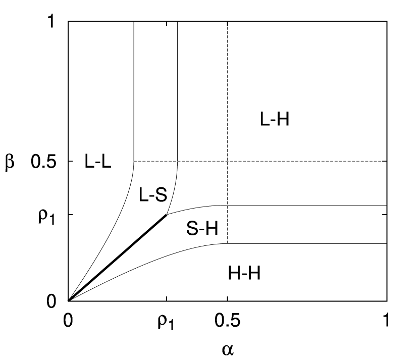
Figure 4: Phase diagram at $\Omega_{A}=2$, $\Omega_{B}=0.4$. Phase boundaries are indicated by solid lines. Letters L,H and S refer to low-density, high-density and localized shock phase, respectively; the first(second) letter refers to lane $A$($B$). The thick solid line indicates the coexistence line. At the dashed lines, the function $J(\alpha,\beta)$ is nonanalytic.

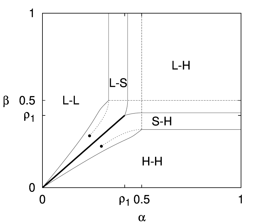
Figure 5: Phase diagram at $\Omega_{A}=2$, $\Omega_{B}=1$. The dotted curves are the discontinuity lines, which terminate at the points indicated by the full circles.

On the other hand, the phase diagrams are richer compared to that of the symmetric model: Besides the phases where the profiles are continuous in the interior of the system, the asymmetry in the lane change kinetics leads to the appearance of phases where one of the lanes contains a localized shock in the bulk. This is reminiscent of the shock phase of the single lane TASEP with Langmuir kinetics. As a new feature, the position of the shock may vary discontinuously with the boundary rates here, when the so-called discontinuity line is crossed. The coexistence line, where coherently moving delocalized shocks emerge in both lanes, is still present, however, it is shorter than in the symmetric case and the shocks walk only a shrunken domain. The subsequent part of the section is devoted to the detailed analysis of these findings.

IV.1 Density profiles

We start the presentation of the results with the description of the density profiles in the phases below the diagonal $\alpha=\beta$ of the two-dimensional phase diagrams.

If the exit rate is small enough, the densities in the bulk exceed the value $1/2$ in both lanes (Fig. 6a). Both profiles are continuous in the bulk and at the exits, i.e. $\lim_{x\to 1}\rho(x)=\lim_{x\to 0}\pi(x)=1-b$, but they are discontinuous at the entrances, i.e. $\lim_{x\to 0}\rho(x)\neq a$ and $\lim_{x\to 1}\pi(x)\neq a$, which signals the appearance of boundary layers on the microscopic scale. The profiles $\rho(x)$ and $\pi(x)$, as well as the current, depend exclusively on $\beta$, while $\alpha$ influences only the boundary layers at the entrances. This situation is observed also in the high-density phase of the TASEP with Langmuir kinetics frey ; ejs , therefore we call this phase H-H phase, referring to the high density in both lanes.

Figure 6: Density profiles in lane $A$ (lower line) and lane $B$ (upper line) for the parameters $\Omega_{A}=2$, $\Omega_{B}=0.4$, $\alpha=0.45$ and for various exit rates: a) $\beta=0.15$, b) $\beta=0.25$, c) $\beta=0.35$ and d) $\beta=0.45$. The profiles in panels a)-c) were obtained by numerically solving eq. (5), whereas those in panel d) are the analytical curves in eq. (14). Results of numerical simulations (dotted lines) obtained for system size $L=10000$ by averaging the occupancies in a period of $10^{7}$ Monte Carlo steps in the steady state are hardly distinguishable from these curves.

In the phase denoted by S-H in the phase diagram, $\rho(x)$ and $\pi(x)$ are continuous at the exits, similarly to the H-H phase, however, the discontinuity in $\rho(x)$ is no longer at $x=0$ but it is shifted to the interior of the system (Fig. 6b). Thus $\lim_{x\to 0}\rho(x)=a$ holds and a shock is located in lane $A$ at some $x_{s}$ ($0<x_{s}<1)$. Therefore this phase is termed S-H phase, where the letter S refers to the shock in lane $A$ and letter H refers to the high density ($\pi(x)>1/2$) in lane $B$. The function $\pi(x)$ is discontinuous at $x=1$, i.e. $\lim_{x\to 1}\pi(x)\neq a$ and it is not differentiable (although continuous) at $x_{s}$. Since both $\rho(x)$ and $\pi(x)$ are continuous at $x=0$, the total current is given by

$$J=a(1-a)-b(1-b)$$ (12)

in this phase. The profile $\rho(x)$ at fixed $\alpha$ and $\beta$ can be computed by substituting the current calculated from eq. (12) into the differential equation (5). Then, the solutions propagating from the left-hand and the right-hand boundary, i.e. the solutions $\rho_{l}(x)$ and $\rho_{r}(x)$ fulfilling the boundary conditions $\rho_{l}(0)=a$ and $\rho_{r}(1)=1-b$, respectively, are calculated numerically. Finally, the position of the shock $x_{s}$ is obtained from the relation $\rho_{l}(x_{s})=1-\rho_{r}(x_{s})$, which is implied by the continuity of the current in lane $A$. Once $\rho(x)$ is at our disposal, $\pi(x)$ can be calculated from eq. (4).

Apart from the discontinuity line to be discussed in the next section, the position of the shock $x_{s}$ varies continuously with the boundary rates in the S-H phase. Fixing $\alpha$ and reducing $\beta$, $x_{s}$ is decreasing and at a certain value of $\beta$, $\beta=\beta_{H}(\alpha)$, the shock reaches the left-hand boundary at $x=0$. At this point, the right-hand solution $\rho_{r}(x)$ extends entirely to the left-hand boundary and a further increase in $\beta$ drives the system to the H-H phase. The phase boundary $\beta_{H}(\alpha)$ between the S-H and the H-H phase is thus determined from the condition $x_{s}=0$ or, equivalently, $\rho_{r}(1)=1-a$. When $\beta$ is increased along a vertical path in the phase diagram at a fixed $\alpha$, $x_{s}$ increases and for $\alpha<\rho_{1}$, where the constant $\rho_{1}$ will be determined later, the path hits the coexistence line before the shock would reach the right-hand boundary (see Sec. III. D). Increasing $\beta$ along a path at some $\alpha>\rho_{1}$, the shock reaches the right-hand boundary at $x=1$ for a certain value of $\beta$, $\beta=\beta_{L}(\alpha)$ and the path leaves the S-H phase. At the phase boundary, the left-hand solution $\rho_{l}(x)$ extends to the whole system and $\rho_{l}(1)=b$ must hold.

Crossing the phase boundary $\beta_{L}(\alpha)$, the L-H phase is entered, where letter L refers to the low density in lane $A$ since here, $\rho(x)<1/2$ and $\pi(x)>1/2$ hold in the bulk (Fig. 6c). In this phase, $\rho(x)$ and $\pi(x)$ are discontinuous at $x=1$, whereas they are continuous at $x=0$ hence the current is given by eq. (12). In the part of the L-H phase where the current is zero, i.e. if $\alpha=\beta$ or $\alpha,\beta\geq 1/2$, the profiles can be calculated analytically. The equal-density solutions of eq. (5) are

$$\ln[\rho_{e}(x)(1-\rho_{e}(x))] = \Omega_{A}(K-1)x+{\rm const},$$

$$\pi_{e}(x) = \rho_{e}(x),$$ (13)

whereas the complementary-density solutions read as

$$\frac{\rho_{1}}{\rho_{2}}\ln|\rho_{c}(x)-\rho_{1}|-\frac{\rho_{2}}{\rho_{1}}\ln|\rho_{c}(x)-\rho_{2}| = 2\Omega_{A}\sqrt{K}x+{\rm const},$$

$$\pi_{c}(x) = 1-\rho_{c}(x),$$ (14)

where the constants $\rho_{1}\equiv 1/(1+K^{-1/2})$ and $\rho_{2}\equiv 1/(1-K^{-1/2})$ are the roots of the equation $S_{A}(\rho,1-\rho)=0$. There is, furthermore, a special complementary-density solution with constant densities:

$$\rho_{c}(x) = \rho_{1},$$

$$\pi_{c}(x) = 1-\rho_{1}.$$ (15)

In the part of the L-H phase where $J=0$, the profiles are given by the complementary-density solution which fulfills the boundary conditions $\rho_{c}(0)=a$ and $\pi_{c}(0)=1-a$ (Fig. 6d).

IV.2 Phase boundaries and the discontinuity line

In the S-H phase (and the L-H phase), the profiles $\rho(x)$ and $\pi(x)$, as well as the current are independent of $\alpha$ if $\alpha\geq 1/2$. Here, $\lim_{x\to 0}\rho(x)=1/2$ and $\alpha$ influences only the microscopic boundary layer, as we argued in Sec. II. As a consequence, the phase boundaries $\beta_{H}(\alpha)$ and $\beta_{L}(\alpha)$ are horizontal lines in the domain $\alpha\geq 1/2$ (see Fig. 4 and 5) and we may restrict the investigation of the phase boundaries to the domain $\alpha\leq 1/2$.

Although we cannot give an analytical expression for the density profiles in general, some information can be gained on the phase boundaries of the S-H phase by investigating the constant solutions of the hydrodynamic equations. A constant solution $\rho(x)=r$, $\pi(x)=p$ must obey $S_{A}(r,p)=0$, otherwise the spatial derivatives $\partial_{x}\rho(x)$ and $\partial_{x}\pi(x)$ would not vanish in eq. (2). On the other hand, the constants satisfy the equation $J=r(1-r)-p(1-p)$, where $J$ is determined by the boundary rates via eq. (12). Eliminating $p$ yields that $r$ is given by the implicit equation:

$$r(r-1)\left[1-\frac{K}{(K+(1-K)r)^{2}}\right]=J(\alpha,\beta).$$ (16)

In the S-H phase, this equation has two roots $r_{1}(J(\alpha,\beta),K)$ and $r_{2}(J(\alpha,\beta),K)$ (shortly $r_{1}$ and $r_{2}$) in the interval $[0,1]$. One can check that for the larger root $r_{2}$, the relation $1/2<1-\beta<r_{2}$ holds, whereas the smaller one, $r_{1}$, may be larger or smaller than $1/2$.

First, we examine the phase boundary separating the L-H phase and the S-H phase. One can check that at this boundary line, $r_{1}<1/2$ holds. Moreover, it follows from eq. (2) that $\frac{d\rho(x)}{dx}>0$ if $0\leq\rho(x)<r_{1}$, and $\frac{d\rho(x)}{dx}<0$ if $r_{1}<\rho(x)<1/2$. Thus, the line $\rho(x)=r_{1}$ behaves as an attractor for the solutions $\rho_{l}(x)$ propagating from the left-hand boundary $x=0$ if $\rho_{l}(0)=\alpha\leq 1/2$, meaning that $\rho_{l}(x)$ approaches monotonously to $r_{1}$ as $x$ increases and $\lim_{x\to\infty}\rho_{l}(x)=r_{1}$. Since $\rho_{l}(x)$ is monotonous and $\rho_{l}(0)=\alpha$, as well as $\rho_{l}(1)=\beta$ hold at the phase boundary, at the common point of the boundary line and the diagonal $\alpha=\beta$, $\rho_{l}(x)$ must be a constant function $\rho_{l}(x)=\alpha$. This, however, implies that $\alpha$ must coincide with $r_{1}$. The endpoint of the boundary line $\beta_{L}(\alpha)$ is therefore at $\alpha=\beta=r_{1}(J=0,K)=1/(1+K^{-1/2})$, which depends only on $K$.

As opposed to this point, the whole function $\beta_{L}(\alpha)$ depends both on $\Omega_{A}$ and $\Omega_{B}$. Nevertheless, we can find an analytical expression for $\beta_{L}(\alpha)$ in the limit $K={\rm const}$, $\Omega_{A}\to\infty$. We can see from eq. (5) that the derivative $\frac{d\rho(x)}{dx}$ is proportional to $\Omega_{A}$ for a fixed $K$. As a consequence, the larger $\Omega_{A}$ is the more rapidly $\rho_{l}(x)$ tends to $r_{1}$. Thus, in the limit specified above, $\lim_{\Omega_{A}\to\infty}(\rho_{l}(1)-r_{1})=0$, which leads to $\beta=r_{1}$. Substituting this into eq. (16), we obtain for the inverse of the boundary curve $\beta_{L\infty}(\alpha)$ in the limit $K={\rm const}$, $\Omega_{A}\to\infty$:

$$[\beta_{L\infty}]^{-1}(\beta)=\qquad\qquad\qquad\qquad\qquad\qquad\qquad\qquad$$

$$\frac{1}{2}\left(1-\sqrt{1-4\beta(1-\beta)\left[2-\frac{K}{\left[K+(1-K)\beta\right]^{2}}\right]}\right).$$ (17)

This curve is plotted in Fig. 7. The phase boundaries obtained by integrating eq. (5) numerically for finite lane change rates tend rapidly to this limiting curve.

Figure 7: Phase boundaries of the S-H phase obtained by integrating eq. (5) numerically for $K=1/5$ and for various $\Omega_{A}$. The solid lines are the limiting curves: $\beta_{L\infty}(\alpha)$, given by eq. (17) and $\beta_{H\infty}(\alpha)$, given solely by eq. (18) since $K<K^{*}$.

Next, we turn to examine the boundary curve between the S-H and the H-H phase, $\beta_{H}(\alpha)$. Along this line, $\rho_{r}(0)=1-\alpha$ and $\rho_{r}(1)=1-\beta$ hold, and the roots of eq. (16) are arranged as $r_{1}<1-\alpha<1-\beta<r_{2}$. One can show that the line $\rho(x)=r_{2}$ is an attractor for the solutions $\rho_{l}(x)$ which start at $x=0$ if $\rho_{l}(0)>\max\{1/2,r_{1}\}$. Moreover, if $r_{1}>1/2$, the line $\rho(x)=r_{1}$ repels the solutions $\rho_{l}(x)$ starting from $x=0$ if $r_{1}<\rho_{l}(0)<r_{2}$, or, in other words, the solutions $\rho_{r}(x)$ propagating from the right-hand boundary, for which $r_{1}<\rho_{r}(1)<r_{2}$, are attracted by the line $\rho(x)=r_{1}$. When the diagonal is approached along the phase boundary $\beta_{L}(\alpha)$, the profile $\rho_{r}(x)$, being monotonous, must tend to the constant function $\rho_{r}(x)=1-\alpha$, as well as $\pi(x)$ since the current is zero at the diagonal. However, equal densities in the two lanes are possible for $K\neq 1$ only if the density is one (or zero), therefore the boundary line must approach the diagonal at $\alpha=0$. This is in accordance with the fact that $r_{2}=1$ if $J=0$. Thus, we obtain $\lim_{\alpha\to 0}\beta_{L}(\alpha)=0$, independently of the lane change rates.

Similarly to $\beta_{L}(\alpha)$, the location of the whole boundary line $\beta_{H}(\alpha)$ depends on both lane change rates (see Fig. 7 and 8) and we can give an analytical expression for $\beta_{H}(\alpha)$ again only in the limit $K={\rm const}$, $\Omega_{A}\to\infty$.

Figure 8: Phase boundaries between the S-H phase and the H-H phase obtained by numerical integration of eq. (5) for $K=1/2>K^{*}$ and for several values of $\Omega_{A}$. The solid lines are the limiting curves given in eq. (18) and eq. (19).

As aforesaid, the profile given by $\rho_{r}(x)$ lies between two attractors, $\rho(x)=r_{1}$ and $\rho(x)=r_{2}$, to which the solutions tend in the limit $x\to-\infty$ and $x\to\infty$, respectively. When $\Omega_{A}$ is increased (such that $K$ is fixed), then $\beta_{L}(\alpha)$ at a fixed $\alpha$ decreases. Thus, the current is increasing and the two roots of eq. (16), $r_{1}$ and $r_{2}$ are coming closer. Keeping in mind that $r_{1}<1-\alpha<1-\beta<r_{2}$, there are now two possible cases. Depending on the value of $\alpha$, either the gap between $1-\beta$ and $r_{2}$ or the gap between $r_{1}$ and $1-\alpha$ vanishes first. In other words, in the former case, the profile is attracted to the line $\rho(x)=r_{2}$ at $x=1$ in the limit $\Omega_{A}\to\infty$, i.e. $\lim_{\Omega_{A}\to\infty}(\rho_{r}(1)-r_{2})=0$, whereas in the latter case it is attracted to the line $\rho(x)=r_{1}$ at $x=0$ (provided that $r_{1}>1/2$) , i.e. $\lim_{\Omega_{A}\to\infty}(\rho_{r}(0)-r_{1})=0$. In the first case, substituting $r=1-\beta$ into eq. (16), we obtain for the inverse of the limiting curve $\beta_{H\infty}^{b}(\alpha)$ in terms of $\beta_{L\infty}(\alpha)$

$$[\beta_{H\infty}^{b}]^{-1}(\beta)=[\beta_{L\infty}]^{-1}(1-\beta),$$ (18)

whereas in the second case, $r=1-\alpha$ yields

$$\beta_{H\infty}^{a}(\alpha)=\qquad\qquad\qquad\qquad\qquad\qquad\qquad$$

$$\frac{1}{2}\left(1-\sqrt{1-\frac{4\alpha(1-\alpha)K}{\left[K+(1-K)(1-\alpha)\right]^{2}}}\right).$$ (19)

These curves are plotted in Fig. 8. The phase boundary in the limit $K={\rm const}$, $\Omega_{A}\to\infty$ is given by

$$\beta_{H\infty}(\alpha)=\max\{\beta_{H\infty}^{a}(\alpha),\beta_{H\infty}^{b}(\alpha)\}.$$ (20)

The value $\alpha^{*}$ at which the functions $\beta_{H}^{a}(\alpha)$ and $\beta_{H}^{b}(\alpha)$ intersect varies with $K$. If $K\to 1$, $\alpha^{*}$ tends to $\frac{\sqrt{3}-1}{2\sqrt{3}}=0.21132\dots$, while $\alpha^{*}=1/2$ if $K$ is equal to

$$K^{*}=1+\sqrt{2}-\sqrt{2(1+\sqrt{2})}=0.21684\dots$$ (21)

Thus, for $K\leq K^{*}$, the limiting curve of $\beta_{H}(\alpha)$ is given by eq. (18) alone, otherwise it is composed of eq. (18) and eq. (19) as given by eq. (20).

Although the curve $\beta_{H\infty}(\alpha)$ gives the phase boundary line only in the limit $K={\rm const}$, $\Omega_{A}\to\infty$, we show that for $K>K^{*}$ and for large enough $\Omega_{A}$, $\Omega_{A}\geq\Omega_{A}^{*}(K)$, the phase transition point at $\alpha=1/2$ is given exactly by eq. (19), i.e. $\beta_{H}(1/2)=\beta^{a}_{H\infty}(1/2)=\frac{K}{1+K}$.

In order to see this, we discuss first the possible appearance of a discontinuity line in the S-H phase, at which the position of the shock $x_{s}$ changes discontinuously. If $r_{1}=1/2$, one can see from eq. (2) that for the spatial derivative of the profile, $\lim_{\rho\to 1/2}\frac{d\rho(x)}{dx}>0$ holds and the left-hand and right-hand solutions $\rho_{l}(x)$ and $\rho_{r}(x)$ may propagate as far as the line $\rho(x)=1/2$. If $\rho_{l}(x_{1})=1/2$ and $\rho_{r}(x_{2})=1/2$ hold for some $x_{1}$ and $x_{2}$, such that $0<x_{1}<x_{2}<1$, then the left-hand and right-hand solutions are connected by a constant segment $\rho(x)=1/2$ in the interval $[x_{1},x_{2}]$ and the profile is continuous (Fig. 9c).

Figure 9: Density profiles for parameters $\Omega_{A}=2$, $\Omega_{B}=1$ and a) $\alpha=0.4$, $\beta=0.29$, where $r_{1}$ is slightly above $1/2$; b) $\alpha=0.4$, $\beta=0.32$, where $r_{1}$ is slightly below $1/2$; c) $\alpha=0.4$, $\beta\approx 0.305$, where $r_{1}=1/2$. d) The endpoint of the discontinuity line at $\alpha\approx 0.297$, $\beta\approx 0.237$.

Substituting $r=1/2$ into eq. (16) we obtain the equation of the discontinuity line: $\alpha(1-\alpha)-\beta(1-\beta)=(\frac{1-K}{2(1+K)})^{2}$, along which the current is constant. Solving this equation for $\beta$, we obtain

$$\beta_{d}(\alpha)=\qquad\qquad\qquad\qquad\qquad\qquad\qquad$$

$$\frac{1}{2}\left(1-\sqrt{1-4\alpha(1-\alpha)+4\left(\frac{1-K}{2(1+K)}\right)^{2}}\right).$$ (22)

This curve is shown in Fig. 5. When at an arbitrary point of this line, $\beta$ is infinitesimally decreased, then $r_{1}$ exceeds the value $1/2$ and a shock appears at $x_{1}$ with an infinitesimal height (Fig. 9a). Conversely, an infinitesimal increase in $\beta$ decreases $r_{1}$ below $1/2$ and an infinitesimal shock appears at $x_{2}$ (Fig. 9b). Thus, when this line is crossed, the position of the shock jumps from $x_{1}$ to $x_{2}$. At the point of the discontinuity line at $\alpha=1/2$, $x_{1}=0$ holds and an infinitesimal increase (decrease) in $\beta$ drives the system to the H-H (S-H) phase. Therefore the point of this curve at $\alpha=1/2$ coincides with the phase boundary, i.e. $\beta_{d}(1/2)=\beta_{H}(1/2)$. On the other hand, comparing eq. (19) and eq. (22), we see that $\beta_{d}(1/2)=\beta_{H\infty}^{a}(1/2)=\frac{K}{1+K}$. The function $\beta_{H\infty}^{a}(\alpha)$ thus gives the phase transition point at $\alpha=1/2$ exactly, provided the curve $\beta_{d}(\alpha)$ is located in the S-H phase. That means if $K>K^{*}$ and $\Omega_{A}\geq\Omega_{A}^{*}(K)$, where $\Omega_{A}^{*}(K)$ is the value of $\Omega_{A}$ at which $\beta_{H}(1/2)$ first reaches the value $\frac{K}{1+K}$, when $\Omega_{A}$ is increased from zero. For example, for $K=1/2$, we have found $\Omega_{A}^{*}(1/2)\approx 0.719$ (Fig. 8). We emphasize, however, that the discontinuity line is lacking if $K<K^{*}$ or $K>K^{*}$ but $\Omega_{A}<\Omega_{A}^{*}(K)$.

If $K>K^{*}$ and $\Omega_{A}>\Omega_{A}^{*}(K)$, then, at the transition point at $\alpha=1/2$, we have $x_{1}=0$; $\Omega_{A}$ influences only $x_{2}$ and $x_{2}\to 0$ if $\Omega_{A}\to\Omega_{A}^{*}(K)$. Moving away from the point at $\alpha=1/2$ along the discontinuity line, the length of the constant segment $x_{2}-x_{1}$ is decreasing and vanishes at a certain point. Here, the density profile becomes analytical and the discontinuity line terminates (see Fig. 9d and Fig. 5). The position of this endpoint depends on $\Omega_{A}$ and it is moving toward smaller values of $\alpha$ for increasing $\Omega_{A}$; in the large $\Omega_{A}$ limit, it tends to the point of intersection of $\beta_{d}(\alpha)$ and $\beta_{H\infty}^{b}$, whereas in the limit $\Omega_{A}\to\Omega_{A}^{*}(K)$, the abscissa of the end point tends to $1/2$.

Finally, we mention that another special curve in the S-H phase is defined by the equation $S_{A}(\alpha,1-\beta)=0$. At this curve the left-hand solution $\rho_{l}(x)$ is constant, therefore both $\rho(x)$ and $\pi(x)$ are constant in the interval $[0,x_{s}]$.

IV.3 Current

We have seen that, apart from the H-H (and the L-L phase), the current is given by eq. (12). It is zero at the line $\alpha=\beta$ and in the domain $\alpha,\beta\geq 1/2$ and it is independent of $\alpha$ ($\beta$) in the H-H (L-L) phase. It is a continuous function of the boundary rates everywhere, although nonanalytic at the boundaries of the H-H phase and the L-L phase, as well as at the lines $\alpha=1/2$ and $\beta=1/2$ outside the H-H phase and the L-L phase, where the effective boundary rates $a$ and $b$ saturate at $1/2$.

In the following, we concentrate on the current in the H-H phase. Since it is continuous at the boundary line $\beta_{H}(\alpha)$, it can be expressed in the H-H phase in terms of $\beta_{H}(\alpha)$ as $J(\beta)=\beta_{H}^{-1}(\beta)(1-\beta_{H}^{-1}(\beta))-\beta(1-\beta)$. According to numerical results (see Fig. 10), the current $J(\beta)$ has a maximum in the H-H phase, and for large $\Omega_{A}$, the location of the maximum tends to $\beta=\beta_{H}(1/2)$ for $K\leq K^{*}$, while for $K>K^{*}$, it tends to $\beta^{*}$ where the curves $\beta_{H\infty}^{a}(\alpha)$ and $\beta_{H\infty}^{b}(\alpha)$ intersect. Contrary to this, the current is a monotonously decreasing function of $\beta$ in the S-H phase.

Figure 10: The current as a function of $\beta$ along the line $\alpha=1/2$ for $K=1/5$ (a) and $K=1/2$ (b). The solid line is the current in the limit $\Omega_{A}\to\infty$, the other curves from bottom to top correspond to $\Omega_{A}=0.25,0.5,1,2,4$, respectively.

We now turn to the question, at which parameter combination the total current is maximal in the steady state. For fixed $K$, the maximal current is realized in the limit $\Omega_{A}\to\infty$ at $\beta_{H\infty}(1/2)$ for $K<K^{*}$ and at $\beta^{*}$ for $K>K^{*}$. Since the current is growing faster in the S-H phase for decreasing $\beta$ than in the H-H phase above $\beta^{*}$ (if $K>K^{*}$), we conclude that the parameter combination that maximizes the current is found in the domain $K<K^{*}$. For $K<K^{*}$, the maximal current is thus $J_{\rm max}(K)=1/4-\beta_{H\infty}(1/2)(1-\beta_{H\infty}(1/2))$. Since $\beta_{H\infty}(1/2)$ decreases monotonously with decreasing $K$, the current is maximal at $K=0$, where $\beta_{H\infty}(1/2)=\frac{2-\sqrt{2}}{4}$ and $J_{\rm max}(0)=1/8$. The value $1/8$ is thus an upper bound for the total current and $J\to 1/8$ in the limit $\Omega_{A}\to\infty$ if $\alpha\geq 1/2$, $\beta=\frac{2-\sqrt{2}}{4}$ and $\Omega_{B}=0$.

Figure 11: The current as a function of $\beta$ in the H-H phase obtained by numerical integration for $K=1/2$ and for different values of $\Omega_{A}$. The analytical approximation given in eq. (23) is indicated by solid lines.

We close this section with the discussion of the current in the H-H phase when the lane change rates are small, i.e. $\Omega_{A},\Omega_{B}\ll 1$. If the vertical hopping processes are switched off, the current is zero, hence we expect that for small lane change rates the current is small, as well. Assuming that $J\ll(\frac{1}{2}-\beta)^{2}$ and expanding the right-hand side of eq. (5) in a Taylor series up to first order in $J$, then solving the resulting differential equation yields finally

$$J=\frac{1-K}{1+K}\beta(1-\beta)(1-2\beta)\times$$

$$\left[\sqrt{1+2(1+K)\frac{\Omega_{A}}{1-2\beta}}-1\right]+\mathcal{O}(\Omega_{A}^{3}).$$ (23)

The details of the calculation are presented in Appendix A. This expression is compared to the current calculated by integrating eq. (5) numerically in Fig. 11. Expanding this expression for small $\Omega_{A}$, we obtain

$$J=\beta(1-\beta)(1-K)\Omega_{A}\left[1-\frac{1+K}{2}\frac{\Omega_{A}}{1-2\beta}\right]+\mathcal{O}(\Omega_{A}^{3}).$$ (24)

The current is thus in leading order proportional to $\Omega_{A}$. Examining the higher-order terms in the series expansion of the right-hand side of eq. (5), one can show that for arbitrary $\Omega_{A}$, the current vanishes as $J\sim 1-K$ when $K\to 1$.

IV.4 Coexistence line

Let us assume that a given point of the section $\alpha=\beta<\rho_{1}$ is approached along a path in the S-H phase. In this case, the position of the shock in lane $A$, $x_{s}$, tends to some $x_{\rm min}=x_{\rm min}(\alpha,\Omega_{A},\Omega_{B})$, which is somewhere in the bulk, i.e. $0<x_{\rm min}<1$. When the same point is approached from the L-S phase, the position of the shock in lane $B$ tends to the same $x_{\rm min}$ according to eq. (7). Thus, when the boundary line $\alpha=\beta<\rho_{1}$ is passed from the S-H phase, the shock in lane $A$ jumps from $x_{\rm min}$ to the right-hand boundary at $x=1$, where a discontinuity appears, while the discontinuity at $x=1$ in lane $B$, which can be regarded as a shock localized there, jumps to $x_{\rm min}$. So, the density profile changes discontinuously. Strictly at $\alpha=\beta$, the shocks in both lanes are delocalized and perform a stochastic motion in the domain $[x_{\rm min},1]$, similarly to the symmetric model with $K=1$ at the line $\alpha=\beta<1/2$.

Now, this phenomenon is investigated in detail in the case of asymmetric lane change. Since the current is zero if $\alpha=\beta$, the solutions of the hydrodynamic equations are those given in eq. (13) and eq. (14) (see Fig. 12).

Figure 12: The flow field of the differential equation (5) for $\Omega_{A}=2$, $\Omega_{B}=0.5$ and $J=0$. The solid curves represent the complementary-density solutions given in eq. (14), whereas dashed curves represent the equal-density solutions given in eq. (13).

The argumentation about the quasistationarity of the fluctuations of the global density presented in the case $K=1$ apply to the case $K\neq 1$, as well. Thus, in the open system, the density profiles averaged over configurations with a fixed global density, $\rho_{\varrho}(x)$ and $\pi_{\varrho}(x)$, can be constructed from the solutions (13) and (14).

Figure 13: Density profiles in lane $A$ (thick solid lines) and in lane $B$ (thick dashed lines) which belong to a fixed global particle density $\varrho$, at four different values of $\varrho$. The flow field of eq. (5) is indicated by thin lines. The rates are $\Omega_{A}=0.5$, $\Omega_{B}=0.25$ and $\alpha=\beta=0.1$.

The structure of these profiles is identical to those obtained in the case $K=1$ (see Fig. 13). Generally, they consist of three segments (see Fig. 13b): An equal-density segment is located in the middle part of the system in the domain $[x_{0},\tilde{x}_{0}]$. This region is connected with the left-hand boundary by a complementary-density segment, which is continuous at $x=0$, i.e. $\rho_{c,l}(0)=\alpha$, $\pi_{c,l}(0)=1-\alpha$, and with the right-hand boundary by another complementary-density segment, which is continuous at $x=1$, i.e. $\rho_{c,r}(1)=1-\alpha$, $\pi_{c,r}(1)=\alpha$. Each lane contains a shock, which are at the opposite ends of the equal-density segment (one at $x_{0}$, the other one at $\tilde{x}_{0}$). The location of the equal-density segment, as well as $x_{0}$ and $\tilde{x}_{0}$ are determined by the actual global density. If $x_{0}=\tilde{x}_{0}\equiv\overline{x}$, the equal-density segment is lacking and $\rho_{c,l}(x)$ and $\rho_{c,r}(x)$ are directly connected by a shock at $\overline{x}$ (Fig. 13c). Since $x_{0}$ and $\tilde{x}_{0}$ are not independent, the shocks move in a synchronized way, and their motion is confined to the range $[x_{\rm min},1]$. If one of the shocks is at $x=1$, the other one is at $x_{\rm min}$, thus, the lower bound $x_{\rm min}$ is determined by the equation $\rho_{c,l}(x_{\rm min})=1-\rho_{e}(x_{\rm min})$, where $\rho_{e}(x)$ is the equal-density solution which fulfills $\rho_{e}(1)=1-\alpha$ (see Fig. 13a). The lower bound $x_{\rm min}$ is an increasing function of $\alpha$ (see Fig 14). In the limit $\alpha\to 0$, $x_{\rm min}$ tends to zero and if $\alpha\to\rho_{1}$, $x_{\rm min}$ tends to 1, thus, at $\alpha=\rho_{1}$, the shock becomes localized at $x=1$ and the system enters the L-H phase. At this point, the density profile is given by the special complementary-density solution: $\rho_{c}(x)=\alpha$, $\pi_{c}(x)=1-\alpha$.

Figure 14: The shock in lane $A$ at the left most possible position for $\Omega_{A}=0.5$, $\Omega_{B}=0.25$ and for different rates $\alpha$($=\beta$).

Similarly to the case $K=1$, the stochastic variation of the global density $\varrho(t)$ is described by a bounded symmetric random walk. The stationary density profile $\rho(x)$ can be obtained from the profile $\rho_{\varrho}(x)$ at a fixed global density by averaging it over $\varrho$. For $K\neq 1$, we could not carry out the averaging analytically, nevertheless, we can gain some information on the stationary density profiles at $\overline{x}$ without the knowledge of the entire profiles. At the point $\overline{x}$, the relation $\rho_{\varrho}(\overline{x})=\pi_{\varrho}(\overline{x})$ holds for all $\varrho$. This, together with the relation $\rho(x)=1-\pi(x)$ following from eq. (7) implies that $\rho(\overline{x})=\pi(\overline{x})=1/2$. As it is shown in Appendix B, the ratio of the first derivatives of the stationary density profile in lane $A$ on the two sides of the point $\overline{x}$ is

$$\frac{d\rho(\overline{x}-)}{dx}/\frac{d\rho(\overline{x}+)}{dx}=\frac{K+(1-K)\rho_{0}}{1-(1-K)\rho_{0}},$$ (25)

where $\rho_{0}\equiv\rho_{c,\alpha}(\overline{x})$. In the case $K<1$, $\rho_{0}<\rho_{1}<1/2$ always holds, hence this ratio is smaller than 1 and the first derivative of the density profile is discontinuous at $\overline{x}$. Furthermore, it is clear that the stationary density profile is identical to the complementary-density solution in the interval $[0,x_{\rm min}]$, since this domain is forbidden for the shocks. We have performed numerical simulations for finite systems of size $L=64,128$ and $256$ and measured the density profiles in the same way as in the symmetric case at the coexistence line. Results are shown in Fig. 15.

Figure 15: Density profiles in lane $A$ obtained by numerical simulations with rates $\alpha=\beta=0.1$, $\Omega_{A}=0.5$, $\Omega_{B}=0.25$ and for different system sizes (thin lines). The thick line represents the density profile $\rho_{\varrho}(x)$ at global density $\varrho=1/2$ in the continuum limit.

V Discussion

In this work, a two-lane exclusion process was studied, where the particles are conserved in the bulk and each lane can be thought of as a totally asymmetric simple exclusion process with nonconserving kinetics in the bulk. As a consequence, the model unifies the features of the particle conserving and bulk nonconserving exclusion processes, as far as the dynamics of the shock is concerned. Namely, it exhibits phases with a localized shock in one lane, while the other one acts as a nonhomogeneous bulk reservoir, the position-dependent density of which is determined by the dynamics itself in a self-organized manner. On the other hand, the model undergoes a discontinuous phase transition at the coexistence line, where delocalized shocks form in both lanes and move in a synchronized way. Here, the global density of particles behaves as an unbiased random walk, similarly to the TASEP at the coexistence line, however, the density profiles in the coexisting phases are not constant here.

Although we considered throughout this work exchange rates proportional to $1/L$, one may imagine other types of scaling. For the TASEP with Langmuir kinetics, shock localization is observed at the coexistence line when the creation and annihilation rates vanish proportionally to $1/L^{a}$ with $1\leq a<2$ js . It might be worth examining whether the synchronization of shocks in the present model persists for lane change rates vanishing faster than $1/L$.

In the limit of large lane change rates, $K={\rm const}$, $\Omega_{A}\to\infty$, the density profiles and the boundaries of the phases exhibiting a localized shock are related to the zeros of the source term in the hydrodynamic equation, which is generally valid for systems with weak bulk nonconserving kinetics frey ; pierobon ; reichenbach . However, different behavior is observed in general when the lane change rates $\omega_{A}$ and $\omega_{B}$ are finite in the limit $L\to\infty$. In this case, the particle current from one lane to the other may be finite at the boundary layers. These currents add to the incoming and/or outgoing currents at the boundaries, which may lead to nontrivial bulk densities even in the case $K=1$, where the profiles are constant.

Possible extensions of the present model are obtained when different exit and entrance rates or different hop rates in the two lanes are taken into account. Nevertheless, these generalized versions are more difficult to treat because of the reduced symmetry compared to that of the present model.

Appendix A

We derive here an approximative expression for the current in the H-H phase in the limit of small lane change rates. Assuming that $J\ll(\frac{1}{2}-\beta)^{2}$, we may expand the right-hand side of the differential equation (5) in a Taylor series up to first order in $J$. Integrating the differential equation obtained in this way yields

$$F(\rho)\equiv\frac{1}{K-1}\ln(\rho-\rho^{2})+J\left\{\frac{K}{(1-K)^{2}}\left[\ln\frac{\rho}{1-\rho}-\frac{1}{\rho}\right]+\right.$$

$$\left.\frac{1}{(1-K)^{2}}\left[\ln\frac{\rho}{1-\rho}+\frac{1}{1-\rho}\right]\right\}=\Omega_{A}x+{\rm const},\qquad$$ (26)

where the first term on the left-hand side is just the equal-density solution for $J=0$. The solution which obeys the boundary condition $\rho(1)=1-\beta$ is $F(\rho)-F(1-\beta)=\Omega_{A}(x-1)$. From this equation, we get for the density at the left-hand boundary, $\rho_{0}\equiv\lim_{x\to 0}\rho(x)$, the implicit equation:

$$F(\rho_{0})-F(1-\beta)=-\Omega_{A}.$$ (27)

On the other hand, we have another relation between $J$ and $\rho_{0}$:

$$J=\rho_{0}(1-\rho_{0})-\beta(1-\beta),$$ (28)

thus, we have closed equations for current. Note that the leading order term on the left-hand side of eq. (27), which comes from the difference of the leading terms of $F(\rho)$ evaluated at $\rho_{0}$ and $1-\beta$, is $\mathcal{O}(J)$, while the next-to-leading contribution in eq. (27) is $\mathcal{O}(J^{2})$. Expressing $\rho_{0}$ from eq. (28) and expanding it for small $J$, we get $\rho_{0}=1-\beta-\frac{J}{1-2\beta}-\frac{J^{2}}{(1-2\beta)^{3}}+\mathcal{O}(J^{3})$. Substituting this expression into eq. (27) gives an implicit equation for $J$. Assuming that $J\ll\beta$ and expanding the terms containing $J$ in this equation in Taylor series, we obtain finally

$$\Theta+\frac{1+K}{2}\Theta^{2}+\mathcal{O}(\Theta^{3})=\frac{\Omega_{A}}{1-2\beta},$$ (29)

where $\Theta\equiv\frac{J}{(1-2\beta)\beta(1-\beta)(1-K)}$. For small $\Theta$, which amounts to $\Omega_{A}\ll 1-2\beta$, we get a good approximation for the current by solving this quadratic equation and arrive at eq. (23).

Appendix B

As we have seen, the positions of the shocks in lane $A$ and lane $B$ are not independent, thus, we may define thereby a function $\tilde{x}_{0}(x_{0})$, which is given implicitly by the equation $\rho_{e}(\tilde{x}_{0})=1-\rho_{c,r}(\tilde{x}_{0})$, where $\rho_{e}(x)$ is the equal-density solution which satisfies the condition $\rho_{c,l}(x_{0})=\rho_{e}(x_{0})$. In the following, we shall denote the density in lane $A$ at $x_{0}$, if the shock is located at $x_{s}$, by $\rho_{x_{s}}(x_{0})$. First, we notice that at the reference point $x_{0}$ ($x_{0}<\overline{x}$), $\rho_{x_{s}}(x_{0})$=$\rho_{c,l}(x_{0})$ holds whenever the shock in lane $A$ resides between $x_{0}$ and $\tilde{x}_{0}(x_{0})$, i.e. $x_{0}<x_{s}<\tilde{x}_{0}(x_{0})$. Similarly, $\rho_{x_{s}}(\tilde{x}_{0}(x_{0}))$=$\rho_{c,r}(\tilde{x}_{0})$ if $x_{0}<x_{s}<\tilde{x}_{0}(x_{0})$. When the shock is outside this interval ($x_{s}\notin[x_{0},\tilde{x}_{0}]$), then $\rho_{x_{s}}(x_{0})$=$\rho_{e}(x_{0})$, where $\rho_{e}(x)$ is some equal-density solution determined by the global density and $\rho_{x_{s}}(x_{0})>1/2$ or $\rho_{x_{s}}(x_{0})<1/2$ if $x_{s}<x_{0}$ or $x_{s}>\tilde{x}_{0}(x_{0})$, respectively. As a consequence of the particle-hole symmetry, the relation $\rho_{x_{s}}(x_{0})=1-\rho_{\tilde{x}_{s}(x_{s})}(x_{0})$ holds if $x_{s}\notin[x_{0},\tilde{x}_{0}]$. Furthermore, in the stationary state, the probability that $x_{s}<x_{0}$ is equal to the probability that $x_{s}>\tilde{x}_{0}(x_{0})$ for any $x_{0}\leq\overline{x}$. Therefore the contribution to the average profile is $1/2$ when $x_{s}\notin[x_{0},\tilde{x}_{0}]$. We can thus write for the average densities at $x_{0}<\overline{x}$ and $\tilde{x}_{0}(x_{0})>\overline{x}$

$$\rho(x_{0})=p(x_{0})\rho_{c,l}(x_{0})+[1-p(x_{0})]\frac{1}{2},$$

$$\rho(\tilde{x}_{0})=p(x_{0}(\tilde{x}_{0}))\rho_{c,r}(\tilde{x}_{0})+[1-p(x_{0}(\tilde{x}_{0}))]\frac{1}{2},$$ (30)

respectively, where $p(x_{0})$ is the probability that the shock in lane $A$ resides in the interval $[x_{0},\tilde{x}_{0}(x_{0})]$, and $x_{0}(\tilde{x}_{0})$ is the inverse function of $\tilde{x}_{0}(x_{0})$. For the spatial derivatives of the densities at $x_{0}$ and $\tilde{x}_{0}(x_{0})$, we get

$$\rho^{\prime}(x_{0})=p^{\prime}(x_{0})\left(\rho_{c,l}(x_{0})-\frac{1}{2}\right)+p(x_{0})\rho_{c,l}^{\prime}(x_{0}),$$

$$\rho^{\prime}(\tilde{x}_{0})=p^{\prime}(x_{0})x_{0}^{\prime}(\tilde{x}_{0})\left(\rho_{c,l}(\tilde{x}_{0})-\frac{1}{2}\right)+p(x_{0}(\tilde{x}_{0}))\rho_{c,r}^{\prime}(\tilde{x}_{0}),$$

where the prime denotes derivation. Using that $p(\overline{x})=0$ and $\rho_{c,l}(\overline{x})=1-\rho_{c,r}(\overline{x})$, we obtain for the ratio of the left- and right-hand side derivatives at $\overline{x}$:

$$\rho^{\prime}(\overline{x}-)/\rho^{\prime}(\overline{x}+)=|\tilde{x}_{0}^{\prime}(\overline{x})|.$$ (32)

Expanding the functions $\rho_{c,l}(x)$, $\rho_{c,r}(x)$ and $\rho_{e}(x)$ in Taylor series up to first order in $x$ around $x=\overline{x}$, we obtain

$$|\tilde{x}_{0}^{\prime}(\overline{x})|=\frac{\rho^{\prime}_{c,l}(\overline{x})-\rho^{\prime}_{e}(\overline{x})}{\rho^{\prime}_{e}(\overline{x})-\rho^{\prime}_{c,r}(\overline{x})}.$$ (33)

Using eq. (2), these derivatives can be given in terms of $\rho_{0}\equiv\rho_{c,\alpha}(\overline{x})$ and we arrive at eq. (25).

- (1) T.M. Liggett Stochastic interacting systems: contact, voter, and exclusion processes, (Berlin, Springer, 1999).
- (2) B. Schmittmann and R. Zia, in Phase Transitions and Critical Phenomena, vol. 17, edited by C. Domb and J.L. Lebowitz (Academic, London, 1995), Vol. 17.
- (3) M.R. Evans, Braz. J. Phys. 30, 42 (2000).
- (4) C. MacDonald, J. Gibbs, and A. Pipkin, Biopolymers 6, 1 (1968).
- (5) For a review, see G.M. Schütz, in Phase Transitions and Critical Phenomena, vol. 19, edited by C. Domb and J.L. Lebowitz (Academic, San Diego, 2001), Vol. 19.
- (6) J. Krug, Phys. Rev. Lett. 67, 1882 (1991).
- (7) B. Derrida, M.R. Evans, V. Hakim and V. Pasquier, J. Phys. A 26, 1493 (1993).
- (8) G. Schütz and E. Domany, J. Stat. Phys. 72, 277 (1993).
- (9) D. Chowdhury, L. Santen, and A. Schadschneider, Phys. Rep. 329, 199 (2000).
- (10) D. Chowdhury, A. Schadschneider, and K. Nishinari, Physics of Life Reviews (Elsevier, New York, 2005), Vol. 2, p. 318.
- (11) J. Howard, Mechanics of Motor Proteins and the Cytoskeleton (Sinauer, Sunderland, 2001).
- (12) R. Lipowsky, S. Klumpp and T.M. Nieuwenhuizen, Phys. Rev. Lett. 87, 108101 (2001).
- (13) S. Klumpp and R. Lipowsky, J. Stat. Phys. 113, 233 (2003).
- (14) M.J.I. Müller, S. Klumpp and R. Lipowsky, J. Phys.: Condens. Matter 17, 3839 (2005).
- (15) R.D. Willmann, G.M. Schütz and D. Challet, Physica A 316, 430 (2002).
- (16) A. Parmeggiani, T. Franosch and E. Frey, Phys. Rev. Lett. 90, 086601 (2003); Phys. Rev. E 70, 046101 (2004).
- (17) V. Popkov, A. Rákos, R.D. Willmann, A.B. Kolomeisky and G.M. Schütz, Phys. Rev. E 67, 066117 (2003).
- (18) M.R. Evans, R. Juhász and L. Santen, Phys. Rev. E 68, 026117 (2003).
- (19) A. Rákos, M. Paessens and G.M. Schütz, Phys. Rev. Lett. 91, 0238302 (2003).
- (20) R. Juhász and L. Santen, J. Phys. A 37, 3933 (2004).
- (21) S. Klumpp and R. Lipowsky, Europhys. Lett. 66, 90 (2004).
- (22) E. Levine and R.D. Willmann, J. Phys. A: Math. Gen. 37, 3333 (2004).
- (23) M.R. Evans, T. Hanney and Y. Kafri, Phys. Rev. E 70, 066124 (2004).
- (24) A. Rákos and M. Paessens, J. Phys. A: Math. Gen. 39 3231 (2006).
- (25) P. Pierobon, T. Franosch and E. Frey, Phys. Rev. E 74, 031920 (2006).
- (26) P. Pierobon, M. Mobilia, R. Kouyos and E. Frey, Phys. Rev. E 74, 031906 (2006).
- (27) H. Hinsch, R. Kouyos and E. Frey, in Traffic and Granular Flow ’05, edited by A. Schadschneider, T. Pöschel, R. Kühne, M. Schreckenberg and D.E. Wolf (Springer, New York, 2006).
- (28) O. Bénichou, A.M. Cazabat, A. Lemarchand, M. Moreau and G. Oshanin, J. Stat. Phys. 97, 351 (1999).
- (29) A.B. Kolomeisky, G.M. Schütz, E.B. Kolomeisky and J.P. Straley, J. Phys. A: Math. Gen. 31, 6911 (1998).
- (30) S. Konzack, P.E. Rischitor, C. Enke and R. Fischer, Mol. Biol. Cell 16, 497 (2005).
- (31) K. Nishinari, Y. Okada, A. Schadschneider and D. Chowdhury, Phys. Rev. Lett. 95, 118101 (2005).
- (32) P. Greulich, A. Garai, K. Nishinari, A. Schadschneider and D. Chowdhury, Phys. Rev. E 75, 041905 (2007).
- (33) H.-W. Lee, V. Popkov and D. Kim, J. Phys. A 30, 8497 (1997).
- (34) V. Popkov and I. Peschel, Phys. Rev. E 64, 026126 (2001).
- (35) V. Popkov and G.M. Schütz, J. Stat. Phys. 112, 523 (2003).
- (36) V. Popkov and M. Salerno, Phys. Rev. E, 69, 046103 (2004).
- (37) V. Popkov, J. Phys. A: Math. Gen. 37, 1545 (2004).
- (38) E. Pronina and A.B. Kolomeisky, J. Phys. A: Math. Theor. 40, 2275 (2007).
- (39) E. Pronina and A.B. Kolomeisky, J. Phys. A: Math. Gen. 37, 9907 (2004); Physica A 372, 12 (2006).
- (40) R.J. Harris and R.B. Stinchcombe, Physica A 354, 582 (2005).
- (41) T. Mitsudo and H. Hayakawa, J. Phys. A: Math. Gen. 38, 3087 (2005).
- (42) T. Reichenbach, T. Franosch and E. Frey, Phys. Rev. Lett. 97, 050603 (2006); T. Reichenbach, E. Frey, and T. Franosch, New. J. Phys. 9, 159 (2007).
- (43) M.J. Lighthill and G.B. Whitham, Proc. R. Soc. London, Ser. A 229, 281 (1955).