Ground-state properties of the one dimensional electron liquid

Abstract

We present a theory of the pair distribution function $g(z)$ and many-body effective electron-electron interaction for one dimensional (1D) electron liquid. Our approach involves the solution of a zero-energy scattering Schrödinger equation for $\sqrt{g(z)}$ where we implemented the Fermi hypernetted-chain approximation including the elementary diagrams corrections. We present numerical results for $g(z)$ and the static structure factor $S(k)$ and obtain good agreement with data from diffusion Monte Carlo studies of the 1D system. We calculate the correlation energy and charge excitation spectrum over an extensive range of electron density. Furthermore, we obtain the static correlations in good qualitative agreement with those calculated for the Luttinger liquid model with long-range interactions.

1 Introduction

Electron-electron interaction is known to produce the most pronounced effects in one dimensional electron liquid (1D EL) systems, where a strongly correlated state appears voit . The effects of interactions in higher than one dimensional systems has been masterfully explained by Landau’s Fermi liquid theory landau dealing with low-lying excitations in a system. Landau called such single-particle excitations quasiparticles and postulated a one-to-one correspondence between the quasiparticles and the excited states of a non-interacting Fermi gas. However, for the 1D EL any individual excitation becomes a collective one. This collectivization of excitations is obviously a major difference between the 1D and higher dimensions electron liquids. It clearly invalidates any possibility to have a Fermi liquid theory in 1D EL. One of the most interesting characteristics of the system is the spin-charge separation seen in a series of remarkable experiments auslaender . Furthermore, according to the theorem proved by Lieb and Mattis lieb , the ground state of a 1D EL is paramagnetic. The recent quantum Monte Carlo calculations malatesta consonant with the Lieb and Mattis theorem predicts no Bloch instability bloch for the 1D EL.

Many of the electron-electron interaction effects become increasingly important as carrier density and dimensionality are reduced and the homogenous electron liquid provides a primitive model for their study. The crucial role in the theory is played by the particle pair distribution function $g(z)$. In our previous works we presented a theory of the pair distribution function and other ground-state properties of the 3D and 2D electron liquid davoudi ; asgari . The theory was based on a Fermi hypernetted-chain approximation (FHNC) which represents a direct generalization to the Fermi systems of the well known hypernetted-chain Euler-Lagrange (HNC/EL) approximation. One of the important feature of theory based on HNC/EL or FHNC is that the theory sums not only all ring and ladder diagrams exactly, but also mixed diagrams in a local approximation jackson . It means the FHNC theory is not a Fermi liquid theory and therefore we able to apply it for studying many-body effects on 1D EL. As we shall see, much higher sophistication is needed to attain a quantitatively useful theory in 1D EL. We shall have to dwell on terms beyond the FHNC/0, which includes elementary diagrams and the three-body Jastrow-Feenberg correlations. These effects have been studied theoretically in boson fluids for the 1D system using the HNC/EL formalism by Krotscheck et al krotscheck .

The main purpose of the present work is the formulation of a practicable theory for charge correlations in the paramagnetic 1D EL and comparison of its numerical predictions with the available diffusion Monte Carlo data casula . The theory is based on variational FHNC lantto80 method made by simplifying the standard FHNC method to have only one Euler-Lagrange Schrödinger equation. The computational time typically needed to obtain $g(z)$ at each value of density is a few minutes on a PC with a Pentium IV/3.4 GHz processor. There are many theoretical works addressing the ground-state properties of the quasi- and strictly gold ; gold1 1D EL but an accurate charge correlations is still missing.

In this work, we numerically study the many-body effects for 1D EL by calculating the pair distribution function and electron-electron effective interactions.

2 Theory

We consider a 1D EL as a model for a system of electronic carriers with band mass $m$ in a semiconductor heterostructure with dielectric constant $\epsilon$. The resulting effective 1D potential is readily shown friesen to be $v(z)=(e^{2}/\epsilon)(\sqrt{2}/2b)~{}exp[z^{2}/4b^{2}]~{}erfc[\left|z\right|/2b]$ with Fourier transform $v(k)=(e^{2}/\epsilon)~{}n~{}exp[b^{2}k^{2}]~{}E_{1}[b^{2}k^{2}]$ where the exponential integral function, $E_{1}(x)$ is defined as $\int_{x}^{\infty}e^{-u}du/u$. The Fourier transform is defined according to the general expression $FT[F(r)]=n\int d{\bf r}F(r)\exp{(i{\bf k}\cdot{\bf r})}$. Here $n$ is the total average density. The above form of the bare potential exhibits the typical 1D behavior, $v(k)\approx ln(kb)$ as $k\rightarrow 0$, and the 3D behavior, $v(k)\approx 1/(kb)^{2}$ as $k\rightarrow\infty$. At zero temperature there are only two relevant parameters for a disorder-free, homogeneous 1D EL in the absence of quantizing magnetic fields, namely the quantum wire width $b$ and the usual Wigner-Seitz density parameter $r_{s}=(2na^{*}_{B})^{-1}$, where $a^{*}_{B}=\hbar^{2}\epsilon/(me^{2})$ is the Bohr radius in the medium of interest. We assume that only one subband is occupied and neglect any contribution from higher subbands. This approximation leads to $r_{s}>\pi b/4$.

With the zero of energy taken at the chemical potential, the formally exact Euler-Lagrange equation for the spin summed pair distribution function $g(z)$ reads lantto ; kallio

$$\left[-\frac{\hbar^{2}}{m}~{}\frac{d^{2}}{dz^{2}}+v(z)+v_{B}(z)+v_{F}(z)\right]\sqrt{g(z)}=0\,.$$ (1)

Here, $v(z)$ is the 1D EL potential and the Bose-like potential $v_{B}(z)$ contains the effects of correlations and by itself would determine $g(z)$ in a Bose fluid. The details of the Bose-like potential have been discussed by many authors, for instance see Ref. [report, ]. We can write it as

$$v_{B}(z)=w_{ind}(z)+\Delta v_{ele}(z)~{},$$ (2)

where the ”induced interaction” is apaja

$$w_{ind}(k)=-\frac{\hbar^{2}k^{2}}{4m}\left[S(k)-1\right]-\tilde{v}_{ph}(k)~{}.$$ (3)

A momentum space formulation of the Euler equations equivalent to Eq. (1) can be written in terms of the structure factor $S(k)$,

$$S(k)=\frac{1}{\sqrt{1+\frac{4m}{\hbar^{2}k^{2}}\tilde{v}_{ph}(k)}}~{},$$ (4)

and the FHNC-Euler-Lagrange theory supplements Eq. (4) with a microscopic theory of the particle-hole interaction report

$$\tilde{v}_{ph}(z)=g(z)[v(z)+\Delta v_{ele}(z)+v_{F}(z)]+\frac{\hbar^{2}}{m}\left|\frac{d}{dz}\sqrt{g(z)}\right|^{2}+[g(z)-1]w_{ind}(z)~{}.$$ (5)

From the theoretical point of view it is important to remark that in FHNC-type calculations at strong coupling the Bose-like $v_{B}(q)$ interactions should be corrected by the addition of three-body correlations and elementary-diagrams (or ”bridge functions”) contributions lantto ; zab ; apaja ; report . The $\Delta v_{ele}(z)$ is a term arising from elementary diagrams and triplet correlations. We only consider the fourth-order elementary diagrams and triplet correlations, $\Delta v_{ele}(k)=w_{B}^{E_{4}}(k)+w_{B}^{(3)}(k)$, which hereafter, we call it as FHNC$/4+$triplet acronym. Note that the approach is reduced to the Fermi hypernetted-chain approximation, FHNC$/0$ when the corrections of the Bose-like interaction are omitted, $\Delta v_{ele}(k)=0$. The contribution from the low-order elementary diagrams to the effective Bose potential is

$$w_{B}^{E_{4}}(k)=-\frac{\hbar^{2}}{4mn}\left\{\frac{k^{2}}{2\pi}\varepsilon_{4}(k)+\int\frac{dq}{(2\pi)}q^{2}[S(q)-1]\frac{\delta\varepsilon_{4}(q)}{\delta S(k)}\right\},$$ (6)

where $\varepsilon_{4}(q)$ is given by a twofold integral (in $1D$) over momentum space.

$$\varepsilon_{4}(q)=\frac{1}{2\,n^{4}}\int\frac{dp\,dq^{{}^{\prime}}}{(2\pi)^{2}}[S(p)-1][S(q^{{}^{\prime}})-1][S(p+q^{{}^{\prime}})-1][S(p+q)-1]~{}[S(p+q^{{}^{\prime}}+q)-1]~{},$$ (7)

and the contribution of three-body correlations is given by the integral,

$$w_{B}^{(3)}(k)=\frac{1}{8n\pi}\int d{q}S(p)S(q)u_{3}({q},{p},{k})\left\{v({q},{p},{k})+\left[\varepsilon(p)+\varepsilon(q)\right]u_{3}({q},{p},{k})\right\}$$ (8)

where ${\bf p}=-({q}+{k})$, $\varepsilon(k)=\hbar^{2}k^{2}/[2mS(k)]$ and, with the definition $X(k)=1-S^{-1}(k)$, we have $v({q},{p},{k})=(\hbar^{2}/m)\left[{k}{p}X(p)+{k}{q}X(q)+{p}{q}X(p)X(q)\right]$ and

$$u_{3}({q},{p},{k})=-\frac{(\hbar^{2}/2m)\left[{k}{p}X(p)X(k)+{p}{q}X(p)X(q)+{k}{q}X(q)X(k)\right]}{\varepsilon(k)+\varepsilon(p)+\varepsilon(q)}~{}.$$ (9)

With regard to the Fermi term $v_{F}(z)$ in Eq. (1), we adopt the same criteria in determining its form as in Ref. [kallio, ]. An important requirement is that Eq. (1) should give the exact fermion distribution function when one goes to the weak-coupling limit $r_{s}\rightarrow 0$, where in this limit $g(z)$ becomes the Hartree-Fock pair distribution function, $g^{\rm\scriptscriptstyle HF}(z)$. The Fermi term in the scattering potential is then determined by the Hartree-Fock structure factor $S^{\rm\scriptscriptstyle HF}(k)$,

$$v_{F}(k)=\frac{\hbar^{2}}{m}{\rm FT}\left[\frac{d^{2}\sqrt{g^{\rm\scriptscriptstyle HF}(z)}/dz^{2}}{\sqrt{g^{\rm\scriptscriptstyle HF}(z)}}\right]+\frac{\hbar^{2}k^{2}}{4m}\left[\frac{S^{\rm\scriptscriptstyle HF}(k)-1}{S^{\rm\scriptscriptstyle HF}(k)}\right]^{2}[2S^{\rm\scriptscriptstyle HF}(k)+1]-\Delta v_{ele}(k)|_{S(k)=S^{\rm\scriptscriptstyle HF}(k)}.$$ (10)

The Hartree-Fock static structure function is given by $S^{\rm\scriptscriptstyle HF}(k)=(k/k_{F})\theta(2k_{F}-k)+\theta(k-2k_{F})$ where $\theta$ is the Heaviside step function, $k_{F}=\pi/4r_{s}a^{*}_{B}$ is the Fermi wave vector and $g^{\rm\scriptscriptstyle HF}(z)$ is given by

$$g^{\rm\scriptscriptstyle HF}(z)=1-\frac{sin^{2}(k_{F}z)}{2\,(k_{F}z)^{2}}~{}.$$ (11)

The rational behind Eq. (10), is as in Ref. [kallio, ], (i) the first term on the RHS ensures that the Hartree-Fock limit is correctly embodied into the theory, (ii) the second and third terms ensure that the Bose-like scattering potential is suppressed for electrons at weak coupling davoudi . We introduce at this point the relation between $g(z)$ and $S(k)$:

$$g(z)=1+\frac{2}{n}\,\int\,cos(k\,z)[S(k)-1]\,dk~{}.$$ (12)

2.1 Sum rules and limiting behaviors

In this section we show that the pair distribution function obtained from the theory presented in Sec. II satisfy three exact properties. These are the behavior of the static structure factor at small momentum, the charge neutrality and the Kimball’s cusp condition.

The asymptotic behavior of the effective potential $v_{ph}(z)$ is first obtained from Eq. (5). A careful analysis of this equation shows that $v_{ph}(z)\rightarrow v(z)+v_{F}(z)$ for $z\rightarrow\infty$, and therefore in Fourier transformation we have $v_{ph}(k)\rightarrow v(k)+\hbar^{2}k_{F}^{2}/m$ for $k\rightarrow 0$, with $v(k)$ as the Fourier transform of bare potentail the 1D EL. The corresponding asymptotic behavior of the structure factor is obtained from Eq. (4), which we have

$$S(k)\rightarrow\frac{\hbar k}{\sqrt{4mv(k)}}~{},$$ (13)

for $k\rightarrow 0$. The analytical behavior of correlations for the 1D EL with long range potential interaction has been obtained by Schulz schulz using the bosonization techniques applied to an effective 1D hamiltonian with linearized kinetic energy expression. According to that model, $S(k)$ behaves like $\propto k/\sqrt{\left|ln(k)\right|}$. It is clear that our scheme gives

$$lim_{k\rightarrow 0}S(k)=k\sqrt{\frac{r_{s}}{4\left|ln(k)\right|}}~{}.$$ (14)

This result agrees with the bosonization findings in 1D. The form of Eq.  (14) immediately ensures that the charge neutrality condition is satisfied. The charge neutrality condition,

$$n\int[g(z)-1]dz=-1~{},$$ (15)

is equivalent to $S(k\rightarrow 0)=0$, a result obtained from Eq. (14). We have numerically evidence that the charge neutrality condition is fulfiled for our total effective potential in Eq. (1). On the other hand, in the small$-r$ limit the bare repulsion potential dominates over the induced plus Fermi potentials. Therefore, it follows from the differential Eq. (1) that

$$g(z\rightarrow 0)=g(0)\left(1+\frac{r_{s}}{12~{}b}\,z\right)~{}.$$ (16)

This is a similar result of the Kimball’s cusp condition kimball for 3D electron gas. Linear small$-z$ behavior together with general properties of Fourier transformations implies that at large $k$ the static structure function $S(k)-1$ approaches zero asymptotically in proportion to $-1/k^{4}$.

2.2 Charge excitations in long-wavelength limit

From the knowledge of static structure factor we can find the behavior of the charge excitations in the long-wavelength limit. Generally, one writes the exact response function as

$$\chi(k,\omega)=\frac{\chi_{0}(k,\omega)}{1-v(k)(1-G(k,\omega))\chi_{0}(k,\omega)}~{},$$ (17)

where $\chi_{0}(k,\omega)$ is the response functiongv_book of the noninteracting 1D EL and the $G(k,\omega)$ is the charge-charge dynamic local-field factor. In this work, we approximate the dynamic local-field factor by its $\omega-$independent, G(k). The charge excitation is determined by calculating the pole of response function. The dispersion relation of charge excitations is given by

$$\omega(k)=\left[\frac{A~{}\beta^{2}_{+}-\beta^{2}_{-}}{(A-1)}\right]^{1/2}~{},$$ (18)

where $A=exp(\pi\hbar^{2}k/mv(k)(1-G(k))$ and $\beta_{\pm}=\hbar(k^{2}/2\pm k_{F}k)/m$.

In the limit $k\rightarrow 0$, the effective potential in momentum space, $v(k)(1-G(k))$ reduce to Fourier transformation of bare potential and $\omega(k)$ turns out to be

$$\hbar\omega(k)=\frac{e^{2}}{a^{*}_{B}}~{}k~{}\sqrt{\frac{\left|ln(k)\right|}{r_{s}}}~{}.$$ (19)

This behavior of the $\omega(k)$ is independent of the statistics due to the exchange potential, $v_{F}(r)$ is of shorter range than $v_{B}(r)$ and essentially the low-momentum limit of $\omega(k)$ remains unaltered. The expression can also be written as:

$$\omega(k\rightarrow 0)=\frac{\hbar k^{2}/2\,m}{S(k)}~{}.$$

On the other hand, the charge oscillation eigenmodes provided by the bosonization model hamiltonian of the Coulomb interaction liquid schulz ; wang is given by

$$\omega_{+}(k)=\frac{\hbar kk_{F}}{m}\,\sqrt{(1+\bar{g_{1}})(1-\bar{g_{1}}+2mv(k)/\pi k_{F})}~{},$$ (20)

where $\bar{g_{1}}=g_{1}k_{F}/2m\pi$ and $g_{1}$ is a nonsingular interaction matrix element at $2k_{F}$. For small $k$ excitations, we have

$$\omega_{+}(k)=\frac{e^{2}}{a^{*}_{B}}\sqrt{1+\bar{g_{1}}}~{}k\,\sqrt{\frac{\left|ln(k)\right|}{r_{s}}}$$ (21)

which is very similar to our finding in Eq. (19).

2.3 Fluctuation-dissipation theorem

In order to calculate the charge excitation spectrum from Eq. (18), the local-field factor is needed. We construct the local-field factor from the fluctuation-dissipation theorem. This theorem, which is of paramount importance for systems in equilibrium, relates the dynamic susceptibility defined above to the static structure factor

$$S(k)=-\frac{1}{\pi}\,\int^{\infty}_{0}d\omega\,\Im[\chi(k,\omega)]~{},$$ (22)

As $\chi(k,\omega)$ depend on $G(k)$ the above integral expression allows one to determine the local-field factor once the static structure factor is calculated. The same approach of obtaining the local-field factor has previously been employed by Iwamoto iwamoto and Dharma-wardana and Perrot dharma-wardana . We note that the use of fluctuation-dissipation theorem to extract static local-field factor is approximate in nature as it neglects the frequency dependence of $G(k,\omega)$ from the outset. However, the apparent success of our previous work in 2D electron gas context asgari_2 also encourages us to use it in the present work.

3 Numerical Results

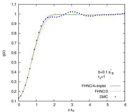
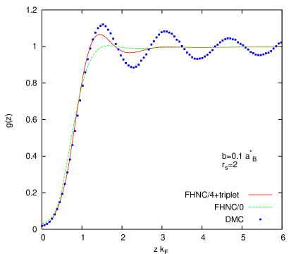
Figure 1: (Color online) The pair distribution function $g(z)$ as a function of $zk_{F}$ for various $r_{s}=1$, ( top panel) and $r_{s}=2$ (bottom panel) at $b=0.1a^{*}_{B}$ comparing the FHNC/0 and FHNC$/4+$triplet approximations with DMC data of Casula et al casula .

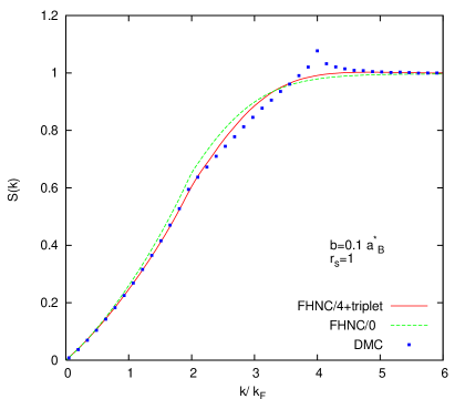
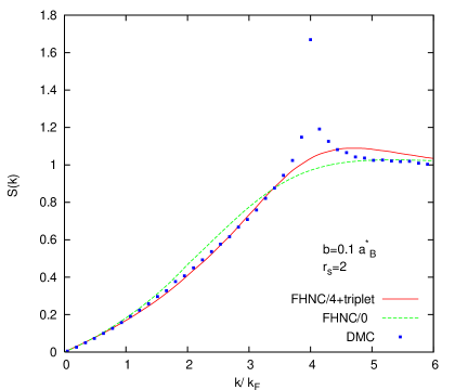
Figure 2: (Color online) The static structure function $S(k)$ as a function of $k/k_{F}$ for $r_{s}=1$ ( top panel), $r_{s}=2$ ( bottom panel) and $b=0.1a^{*}_{B}$ comparing both FHNC/0 and FHNC$/4+$triplet approximations with DMC data of Casula et al casula .

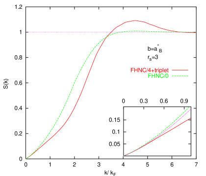
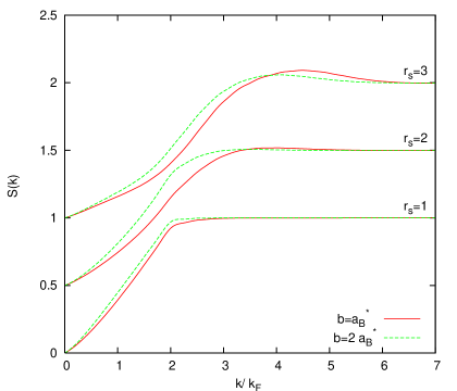
Figure 3: (Color online) Top: The static structure function $S(k)$ as a function of $k/k_{F}$ for $r_{s}=3$ at $b=a^{*}_{B}$ calculating within both FHNC/0 and FHNC/4$+$triplet approximations. In the inset the long-wavelength behavior of $S(k)$ is shown in comparison with sum rule relation (dotted curve). Bottom: The static structure function $S(k)$ as a function of $k/k_{F}$ for different $r_{s}$ and $b$ values calculating within FHNC$/4+$triplet approximation. The curves at $r_{s}=2$ and 3 have been shifted upwards by 0.5 and 1.0, respectively.

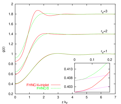
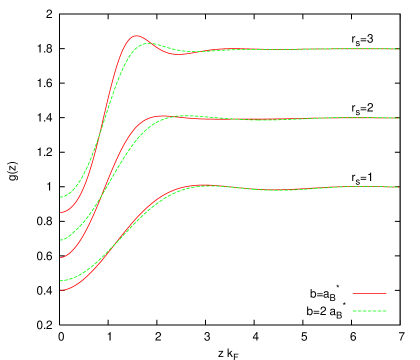
Figure 4: (Color online) Top: The pair distribution function $g(z)$ as a function of $zk_{F}$ for various $r_{s}$ values at $b=a^{*}_{B}$ calculating within both FHNC/0 and FHNC$/4+$triplet approximations. In the inset the cusp condition is shown (dotted curve). Bottom: The pair distribution function $g(z)$ as a function of $zk_{F}$ for different $r_{s}$ and $b$ values calculating within FHNC$/4+$triplet approximation. The curves at $r_{s}=2$ and 3 have been shifted upwards by 0.4 and 0.8, respectively.

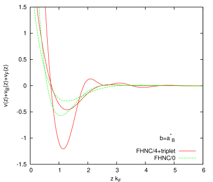
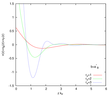
Figure 5: (Color online) Top: The total potential $v(z)+v_{B}(z)+v_{F}(z)$ as a function of $zk_{F}$ for $r_{s}=2$ and $3$ values at $b=a^{*}_{B}$ calculating within both FHNC/0 and FHNC$/4+$triplet approximations. Note that deeper potential refer to large $r_{s}$ value. Bottom: The total potential $v(z)+v_{B}(z)+v_{F}(z)$ as a function of $zk_{F}$ for various $r_{s}$ at $b=a^{*}_{B}$ calculating within FHNC$/4+$triplet approximation. Deeper potential indicate larger $r_{s}$ value.

We turn to a presentation of our numerical results, which are obtained by solving Eq. (1) with the following self-consistency cycle. We start with the trial choice $g(z)=g^{\rm\scriptscriptstyle HF}(z)$ and $v_{B}(z)=0$, and find the effective potentials $\tilde{v}_{ph}(z)$ by means of Eq. (5) and hence the structure factor $S(k)$ via Eq. 4. At this point we can calculate new values for $g(z)$ and for $v_{B}(z)$ by taking Fourier transforms and using Eqs. (2) and (3). This procedure is repeated until self-consistency is achieved. We have calculated in this way the pair distribution function of a 1D EL for various $r_{s}$ and $b$ values. The main results of our work are shown in Figures 1-6.

Our numerical results of the pair distribution function of the 1D EL is compared with the DMC data of Ref. [casula, ] in Figure 1. The quantum wire width is $b=0.1a^{*}_{B}$ and the system is highly correlated. We have clearly achieved good qualitatively agreement with the DMC data. It is obvious from the Fig. 1, FHNC$/4+$triplet results are in excellent agreement with DMC data up to $zk_{F}<1.3$ and less agreement in larger $z$-values to produce the oscillation behavior. The strong oscillation behavior in DMC data corresponds to the periodicity of the quasi-Wigner crystal. It is apparent from the figure that FHNC$/4+$triplet approach which includes further corrections than FHNC/0, modifies the results and show the first peak and its oscillatory behavior, however the magnitude of peak is less than the one predicted by DMC simulation. Our $g(z)$ has more structure within FHNC$/4+$triplet than the $g(z)$ obtained within FHNC/0. Moreover, in both approaches the short-range behavior of $g(z)$ give correct shape in base on Kimball’s cusp condition and they have different values at contact.

In Figure 2, we show our results for $S(k)$ in the paramagnetic 1D EL at $r_{s}=1$ and $2$ within both FHNC$/0$ and FHNC$/4+$triplet approximations. It is obvious to see the improvements brought above by the use of FHNC$/4+$triplet over FHNC/0. Apart from the strong peak structure at $q=4k_{F}$ which appears in DMC simulation, the FHNC$/4+$triplet results are in good agreement with the DMC data of Casula et al casula . The strong peak has been related to a quasi-order of the electrons schulz ; casula . Note that there is no true long-range order in 1D system. We find that as the density is reduced the correlation effects become stronger and $S(k)$ starts to develop a broad peak around $q=4.5k_{F}$. The FHNC$/0$ does not show any peak as the density decreases. Theory gives the correct behavior of the long-wavelength limit of $S(k)$ and the results coincide with the DMC data.

There are several noteworthy points based on the results shown in Figs. 1 and 2. (i) Despite that FHNC gives very good results for the pair distribution function and static structure factor in high dimensional electron liquids davoudi ; asgari ; lantto80 ; zab , it can give qualitative results for 1D EL where the system is highly correlated. (ii) The approach could not produce a strong peak for static structure factor at $q=4k_{F}$ which is related to the slow decay of the $4k_{F}$ components of the charge density-density correlation function.

In order to emphasize the effect of correlations at strong coupling regime, we display in Fig. 3 the static structure factor obtained within both FHNC$/0$ and FHNC$/4+$triplet approximations. The strong coupling arises with decreasing either the density of electrons or the quantum wire width parameter $b$. $S(k)$ move towards right in intermediate of momenta value and starts to develop a broad peak around $q=4.5k_{F}$ within the FHNC$/4+$triplet approach. In the inset of the Fig. 3a, the behavior of the long-wavelength limit of $S(k)$ both in FHNC/0 and FHNC$/4+$triplet approximation are shown in comparison with sum-rule given by Eq. (14). As the sum-rule of the long-wavelength limit of $S(k)$ is proven in the based on our approach, we numerical evidence that this sum-rule is fulfilled. It is apparent from Fig. 3b that by reducing the $b$ value, the peak moves towards right and the magnitude of the peak becomes larger for the same $r_{s}$ value.

The corresponding pair distribution functions are shown in Fig. 4. Again, we show the effect of correlations which are corrected by including further correction functions to the Bose potential within the FHNC$/4+$triplet approximation. The value of $g(0)$ decreases with decreasing either the density $n$ or $b$ values, but its value always remains positive, consistent with the probabilistic definition. Moreover, In the inset of the Fig. 4a, the behavior of the short range limit of $g(z)$ both in our approaches are shown in comparison with cusp condition. Note that the $g(0)$ value at contact is dependence the approach. We numerical evidence that the cusp condition is fulfilled.

In Fig. 5 we report the effective electron-electron interaction $v(z)+v_{B}(z)+v_{F}(z)$ as it emerges from our self-consistent calculations on a 1D EL. The attractive part of the effective interaction deepens with increased $r_{s}$ or decreased $b$, as is physically expected. Moreover, its deepens in more larger in FHNC$/4+$triplet than FHNC/0.

After reaching good agreement between the static structure factor with data from diffusion Monte Carlo, we can then calculate the correlation energy per particle $\varepsilon_{c}(r_{s})$, the difference between the exact ground-state energy and the sum of the noninteracting kinetic energy and the exchange energy, of the 1D EL as a function of $r_{s}$, using an integration over the coupling strength according to the expression

$$\varepsilon_{c}(r_{s})=\frac{1}{2}\int_{0}^{1}\frac{d\lambda}{\lambda}~{}\int\frac{dk}{2\pi}~{}v^{(\lambda)}_{k}~{}[S_{\lambda}(k)-S^{\rm\scriptscriptstyle HF}(k)]~{},$$ (23)

(in Rydberg units). Here the static structure factor $S_{\lambda}(k)$ calculated with interaction $v^{(\lambda)}_{k}=\lambda(e^{2}/\epsilon)~{}exp[b^{2}k^{2}]~{}E_{1}[b^{2}k^{2}]$. We have calculated the correlation energy for $b=a^{*}_{B}$ and $2a^{*}_{B}$ over the range $0.1\leq r_{s}\leq 4$. The results are reported in Table I in comparison with DMC data from Casula et al. casula The Table also include other theoretical results obtained in the self-consistent dielectric theory of Singwi et al. stls with an analytical form of the local-field factor from Calmels and Gold. gold

It is seen from Table that the present theoretical approach yields fairly better accurate values of the correlation energy respect to the Calmels and Gold results gold .

Finally, in Fig. 6 we display the charge excitation spectrum obtained within the FHNC$/4+$triplet approximation. The $\omega(k)$ behaviors like $k\sqrt{\left|lnk\right|}$ at long-wavelength limit and reaches to the particle-hole continuum boundary which is given by $\beta_{+}$ in the large $k$-limit. We use the local-field factor which is calculated from the fluctuation-dissipation theorem by Eq. (22). The local-field factor should be useful to study many physical characteristics using a suitably defined the dielectric function.

4 Summary

In summary, we have presented in this work a theoretical study of the pair distribution function, the effective electron-electron interaction and the correlation energy of the 1D electron liquid where the system is strongly correlated. Our approach yields numerical results of good agreement in comparison with recent diffusion Monte Carlo studiescasula . We showed that the long-wavelength behavior of the static structure factor is in agreement with the bosonization findings for the Coulomb Luttinger liquid. The charge excitation spectrum is calculated and it is expected to give better results when compared to experimental measurements in intermediate $r_{s}$ values and even large momentum limit where the Random Phase approximation calculation is no longer accurate. Moreover, the small $k$ behavior of the charge excitation spectrum is shown be equivalent with the bosonization findings. Improvements of the theory will be necessary for a quantitative study of the physical quantities and the correlation energy. As we have mentioned in the main text, we only considered the low-order elementary diagrams and the three-body corrections in the theory is based on Fermi hypernetted-chain approximation. We believe inclusion of the contributions of the fifth-order and higher elementary diagrams will improve our results. Moreover as we mentioned in the main text, we used a practical recipe of FHNC approach lantto by replacing Jastrow product factor to the square of the Slater determinant describing the non-interacting fermions gas wave-functions. This recipe of FHNC reduces correlation respect to the full FHNC-EL theory. Although it is little affect in high dimensions but it may be important in the specific case of a 1D EL.

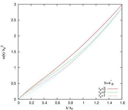
Figure 6: (Color online) The charge excitation spectrume $\omega(k)$ as a function of $k/k_{F}$ for various $r_{s}$ values at $b=a^{*}_{B}$ obtaining from Eq. (22) within the FHNC$/4+$triplet approximation. Dashed-dotted curve indicates the boundary of particle-hole continuum, $\beta_{+}$ .

Table 1: Correlation energy of the 1D EL in Ryd/electron. DMC from Casula, casula STLS from Calmels and Gold gold

. $r_{s}$ Various calculations $b=a^{*}_{B}$ $b=2a^{*}_{B}$ 0.1 DMC -0.000463 -0.000110 Present work -0.000459 -0.000107 STLS -0.000457 -0.000117 0.2 DMC -0.0016996 -0.000418 Present work -0.001665 -0.000411 STLS -0.001645 -0.000431 0.4 DMC -0.00579 -0.001514 Present work -0.00564 -0.001502 STLS -0.005449 -0.001492 0.6 DMC -0.01122 -0.003089 Present work -0.01099 -0.002983 STLS -0.01044 -0.002955 0.8 DMC -0.01738 -0.00498 Present work -0.01678 -0.00476 STLS -0.01608 -0.00469 1.0 DMC -0.02394 -0.00709 Present work -0.02296 -0.00687 STLS -0.02202 -0.00662 2.0 DMC -0.05840 -0.01912 Present work -0.05311 -0.01806 STLS -0.04968 -0.01735 3.0 DMC -0.0856 -0.0322 Present work -0.07330 -0.02952 STLS -0.06862 -0.02744 4.0 DMC -0.09986 -0.04372 Present work -0.08518 -0.03814 STLS -0.07978 -0.03556